Random Field Potts model with dipolar-like interactions: hysteresis, avalanches and microstructure

Abstract

A model for the study of hysteresis and avalanches in a first-order phase transition from a single variant phase to a multivariant phase is presented. The model is based on a modification of the Random Field Potts model with metastable dynamics by adding a dipolar interaction term truncated at nearest neighbors. We focus our study on hysteresis loop properties, on the three-dimensional (3D) microstructure formation and on avalanche statistics.

I Introduction

Microstructure formation in first-order phase transitions is a phenomenon that has been studied by physicists, mathematicians and engineers Salje (1990); K.Bhattacharya (2003); Khachaturyan (1983). It is important not only from a fundamental point of view, but also for applications, due to its relationship with material properties. Microstructures occur in ferroic systems (ferromagnetic, ferroelectric and/or ferroelastic) which are driven through a first-order phase transition (FOPT) in which some symmetry operations of the parent phase are lost. The product phase (usually less symmetric) may appear in energetically equivalent variants which are related by the symmetry operations that have been lost in the transition. The obtained microstructures correspond to the arrangement of such equivalent variants and are decided by the interplay of many energetic terms: interface energy, surface energy and long-range interactions.

Until now many of the studies on microstructures have focused on the determination of the optimal variant configuration minimizing a certain thermodynamic potential that takes into account the above factors and external conditions. Nevertheless, in many cases, when real materials are studied, such optimal microstructures are not observed. This is mainly due to two important factors: (i) the existence of disorder sources of very different natures both in the bulk and on the surfaces and also (ii) the athermal character of the phase transition dynamics: when the temperature is not very high, the energetic barriers that separate the optimal solutions from the parent phase cannot be overcome. Thus, the system evolves following metastable paths which locally optimize the system energy, but are far from the trajectories obtained from a global minimization principle. An interesting suggestion on the behavior of microstructure formation comes from the glass-jamming transition framework (see Refs. Toninelli et al., 2006; Toninelli and Biroli, 2006 and references therein), which is associated with the so-called kinetically constrained model. These models are stochastic lattice gases with hard core exclusion, with the addition of some local constraints, which mimic the geometric constraints on the possible rearrangements in physical systems. Similar behavior is quite likely to arise in microstructure formation.

The use of continuum models derived from elasticity theory R.Ahluwalia and G.Ananthakrishna (2001); Jacobs et al. (2003); D.M.Hatch et al. (2003); T.Lookman et al. (2003); K.Ø.Rasmussen et al. (2001) has been proposed as another approach to microstructure formation. Some of these models have been successful in explaining microstructures, hysteresis and avalanches. Nevertheless, they are very time consuming from a computational point of view. For this reason, in many cases only 2D problems have been addressed, and even this item presents difficulties connected with large statistics and with the scanning of the model parameters in order to study their influence. Our aim here is to find a statistical mechanical lattice model, easy to simulate and which allows for the study of statistics of microstructure sequences dynamically generated in athermal systems, under the influence of disorder.

The Random-Field Ising model (RFIM) Sethna et al. (1993) with metastable dynamics is one of the simplest models for the study of the combined effects of disorder and athermal evolution. It is formulated in a magnetic language for a spin reversal transition, driven by an external magnetic field $H$. The only degrees of freedom are spin variables defined on a lattice $(i=1,...,N)$, which take values $S_{i}=\pm 1$ on the $i$-th lattice site. The RFIM enables computation of hysteresis loops $M(H)$ corresponding to the behavior of the order parameter $M=\sum_{i}S_{i}$ as a function of $H$ as well as the analysis of the intermediate states between the negatively saturated initial state $\{S_{i}=-1\}$ and the final positively saturated state $\{S_{i}=+1\}$, and vice versa. In particular, the RFIM has been successful in understanding the avalanche dynamics (Barkhausen noise H.Barkhausen (1919)) that joins the intermediate metastable states and shows absence of characteristic scales for a critical amount of disorder. Moreover, the RFIM displays several other interesting properties Sethna et al. (1993); Dhar et al. (1997): it exhibits a well-defined rate-independent trajectory, it shows return point memory, it satisfies the abelian property and, from a computational point of view, it is fast to simulate trajectories in relatively large systems Kuntz et al. (1999).

Nevertheless, the usefulness of the RFIM for the study of microstructures is almost null. This happens because the parent and product phases in the RFIM are the positively magnetized phase and the negatively magnetized phase. These two phases are single variant and totally equivalent from a symmetry point of view. Consequently, the obtained hysteresis loops are symmetric under the exchange $H\rightarrow-H$ and $M\rightarrow-M$, there is absence of latent heat associated with the FOPT and the domains are spherically symmetric (except for some short-range correlations due to lattice symmetries).

Within this framework, the aim of the present work is to explore some modifications that should be introduced in the RFIM in order to obtain 3D microstructures without losing, as far as possible, some of the useful RFIM properties that we have mentioned above. A first step in this direction was done several years ago by defining the Random Field Blume-Emery-Griffiths model, in which the ’spin’ variables take three different values ($S_{i}=-1,0,1$) with metastable dynamics E.Vives et al. (1995). In this case, the FOPT takes place from a single variant parent phase, represented by $S_{i}=0$, and a product phase with two variants $S_{i}=+1$ and $S_{i}=-1$. In the cited work, the hysteresis loops, phase diagram and avalanche distribution were studied for this type of simple case. In the present paper we would like to go one step forward. This will be done by starting from the Random Field Potts model Blankschtein et al. (1984) with metastable dynamics. In the Potts model the spin variables can take an arbitrary number of values. This model allows phase transitions to be studied from a non-degenerate phase $S_{i}=0$ to a multivariant product phase. We will explore the effect of an extra interaction term (of a dipolar nature, but truncated to the nearest-neighbor approximation), which will be necessary in order to produce microstructures (for the introduction of dipolar interactions in RFIM, see Magni (1999)). It is not our aim to focus on the detailed analysis of any particular transition. We will study a model that, from the point of view of symmetry, would correspond to a transition from a cubic phase (single variant) to a tetragonal phase (with three equivalent variants), although neither the detailed interactions nor the external constraints will be tuned for the particular modeling of such transitions in ferroelastic systems. This will be the aim of a future work .

The paper is organized as follows: in section II we introduce the hamiltonian of the model. In section III we detail the metastable dynamics that has been used for the simulations. Section IV is devoted to the discussion of the obtained results: in section IV.1 we present our analysis on the shape of hysteresis loop cycles as a function of the model parameter values. In this section it is shown that the loops happen to be unsymmetric, in contrast to the RFIM results. The microstructures are analyzed in section IV.2, where we discuss three different regimes corresponding to different ranges of the parameters values. Moreover, in section IV.3 we present the statistical analysis of avalanche behavior. Finally, we summarize and discuss the future perspectives in section V.

II Model

The model can be defined on any regular lattice. We will consider a simple cubic lattice of size $N=L\times L\times L$ with periodic boundary conditions. At each lattice site we define a variable $S_{i}$ ($i=1,\dots N$), which can take four different values that we will call $0$, $x$, $y$ and $z$. We can choose different representations for our variables but it is convenient to consider a vector $\vec{S_{i}}$ having three components: we will indicate the four possible values as $0=(0,0,0)$, $x=(1,0,0)$, $y=(0,1,0)$ and $z=(0,0,1)$.

The order parameter for the phase transition under study here is $M=\sum_{i}(\vec{S}_{i})^{2}$, where the sum spans over the whole lattice. $M$ represents the amount of the system that has transformed from the cubic to the tetragonal phase. By following the analogy with the magnetic case, we will refer to $M$ as the total magnetization of the system. Moreover, we define the normalized magnetization $m$, as $m=M/N$. We will drive the system by an external field $H$ coupled to $M$, since we are interested in the transition from the $0$ phase to the multivariant phase which will be composed of regions (variants) in the states $x$, $y$ and $z$. The field $H$ would correspond to the driving effect of the temperature in athermal structural transitions. We will start by decreasing $H$, from the $M=0$ state. We consider the following hamiltonian:

$${\cal H}=-k\sum_{<ij>}^{NN}\delta(\vec{S}_{i},\vec{S}_{j})+\lambda\sum_{<ij>}^{NN}\frac{(\vec{S}_{i}\cdot\vec{r}_{ij})(\vec{S}_{j}\cdot\vec{r}_{ij})}{|\vec{r}_{ij}|^{3}}\\ +H\sum_{i}^{N}(\vec{S}_{i})^{2}+{\cal{H}}_{dis}$$ (1)

The first term is a Potts exchange term extending to nearest-neighbor (n.n.) pairs. The parameter $k$ will be always positive, favoring the ferromagnetic interaction between spins in the same state. In the following, without loss of generality, we will consider $k=1$.

The second term is a dipolar interaction truncated to n.n. pairs. As we have already said, the aim of adding this term is to generate some simple microstructures. To include higher order terms would lead to more realistic ones. The vector ${\vec{r}}_{ij}$ is the lattice vector joining ’spins’ ${\vec{S}}_{i}$ and ${\vec{S}}_{j}$. We will study the cases with $\lambda<0$ and $\lambda>0$ separately. As can be easily seen from Eq. 1, in fact, the $\lambda<0$ case corresponds to favoring the growth of prolate (needle-like) domains parallel to the spin direction. On the other hand, for $\lambda>0$ such a growth is not favored, but as it is partially compensated by the exchange term it basically corresponds to the formation of oblate (disk-like) domains, perpendicular to the spin direction. We will illustrate these features in Sec. IV.2.

The third term of the hamiltonian accounts for the interaction between the system and the external field $H$. This field will be driven from very high positive values to very negative values (and vice versa) in steps $\Delta H$, mimicking an adiabatic triangular driving force (i.e. field frequency $\omega\rightarrow 0$). By a deliberate abuse of language we will refer to the step $\Delta H$ as the driving rate. One can notice that it is possible to add a second driving term $\vec{G}\sum\vec{S}_{i}$ which would be convenient for the study of the transitions from one variant to another, mimicking, for instance, the effect of an applied external stress.

The last term ${\cal{H}}_{dis}$ accounts for the quenched disorder of the system. We will restrict ourselves to a random field type with zero averages. However, there are still several possibilities for such a hamiltonian term because the random fields can couple either to $\vec{S}_{i}$ or to the order parameter $(\vec{S}_{i})^{2}$. We will thus consider:

$${\cal{H}}_{dis}=\sigma\sum_{i}^{N}\vec{g}_{i}\cdot\vec{S}_{i}+\rho\sum_{i}^{N}{h}_{i}(\vec{S}_{i})^{2}$$ (2)

where $\vec{g}_{i}$ is a three-component vector random field, whose components are extracted from a gaussian distribution $N(0,1)$ with zero mean and unitary standard deviation, and ${h}_{i}$ is a scalar field, again extracted from a gaussian distribution $N(0,1)$. The parameters $\sigma$ and $\rho$ control the amount of quenched disorder in the system.

In order to compare our model with the standard RFIM, we define the total amount of disorder $\sigma_{0}^{2}=\sigma^{2}+\rho^{2}$. In practice, the two disorder terms can be understood as arising from a local random field $\vec{f}_{i}$, whose components are correlated, being

$$\vec{f}_{i}=\sigma(g_{ix},g_{iy},g_{iz})+\rho(h_{i},h_{i},h_{i}),$$ (3)

so that $\langle f_{ix}^{2}\rangle=\langle f_{ix}^{2}\rangle=\langle f_{ix}^{2}\rangle=\sigma_{0}^{2}$ and $\langle f_{ix}f_{iy}\rangle=\langle f_{ix}f_{iz}\rangle=\langle f_{iy}f_{iz}\rangle=\rho^{2}$.

III Dynamics

There are several possibilities for the choice of metastable dynamics. In Fig. 1 we show examples of hysteresis loops obtained with three possible choices of dynamics. At first sight, the three loops look very similar. In all the cases we start from a metastable state, we increase or decrease the field by a $\Delta H$ step and then, at constant field, we recursively minimize the system energy by using a local rule based on single-spin changes. Only after a new metastable state is reached we proceed with a new field change $\Delta H$.

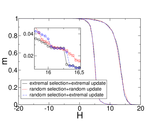
Figure 1: (Color on line) Hysteresis cycles for three different dynamics as explained in the text. The parameters of the simulations are: $\Delta H=0.05$, $L=16$, $\lambda=-10$, $\sigma=5$ and $\rho=2$. In the inset: a magnification of a loop region: the magnetization values for the three dynamics coincide only for some field values.

In the extremal selection + extremal update case, we scan the whole system and check which variable $S_{i}$ can change to a new value with the minimum energy difference $\Delta{\cal H}$. The proposed change is accepted if this minimum $\Delta{\cal H}$ is negative. In the random selection + random update case, we randomly choose a spin on the lattice and propose a random change to a new value. If the proposed change implies $\Delta{\cal H}<0$ the change is accepted. Finally, in the random selection + extremal update dynamics, we randomly choose a spin on the lattice and check among the three possible new values which one represents a minimum $\Delta{\cal H}$. If this minimum value is negative we accept the change. From a computational point of view the first choice is much more time consuming than the other two, since the effort scales with $L^{3}$.

Although the loops are very similar, detailed analysis reveals that the obtained hysteresis loops, as well as the sequence of metastable states, are not identical. This tells us that the proposed model is not abelian and that the final state will depend on the order in which unstable spins will be changed. In order to ensure some robustness of the results, we are thus forced to choose extremal selection + extremal update dynamics, that is: to propose the optimal spin change among the whole lattice and among all the three possible final values at each time step. This kind of dynamics is deterministic and thus, by definition, independent of the updating order. We will keep to this dynamics for the rest of the paper.

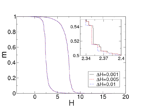
Figure 2: (Color on line) Hysteresis cycles for various values of the applied field rate $\Delta H$ with the extremal selection+extremal update dynamics. The parameters of the simulations are: $L=16$, $\lambda=-5$, $\sigma=4$ and $\rho=0$. In the inset: a magnification of a portion of the hysteresis cycle.

We now study the effect of changing the value of $\Delta H$. In Fig. 2 we show three hysteresis cycles obtained for different values of the driving rate $\Delta H$ using the extremal selection+extremal update dynamics. A detailed analysis reveals that the differences between the three loops can be attributed to the fact that driving with a smaller $\Delta H$ allows more metastable intermediate states to be found, but for the same applied field values, in the three realizations not only the magnetization, but also the final microscopic configurations reached are the same. The independence from the field rate is an important property from the point of view of the simulations, since it allows us to use a relatively large $\Delta H$ for the study of the properties of hysteresis loops.

IV Results

We have performed numerical simulations of systems with sizes $L=8,16,32,40$ and $60$, averaging over $10^{2}-10^{3}$ realizations of the quenched random fields. We have focused our analysis on hysteresis loops behavior, on microstructure formation and on the statistical properties of the avalanches.

IV.1 Hysteresis loops

In Figs. 3, 4 and 5, we show some examples of hysteresis loops simulated with our model in order to illustrate the effect of the different hamiltonian parameters.

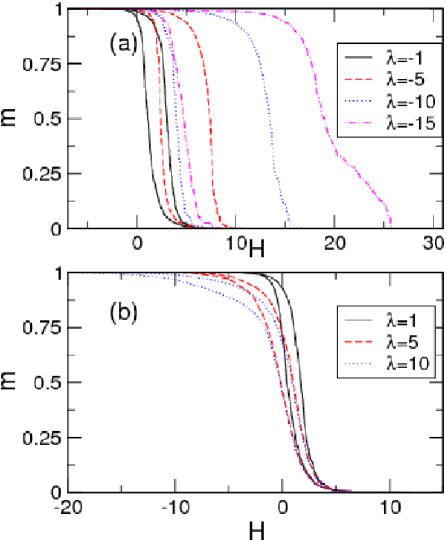
Figure 3: (Color on line) Examples of hysteresis loops for different values of the parameter $\lambda$: (a) $\lambda=-1,-5,-10,-15$ and (b) $\lambda=1,5,10$. In all the cases, $L=16$, $\Delta H=0.01$, $\sigma=3$ and $\rho=0$

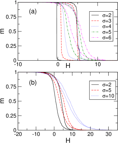
Figure 4: (Color on line) Examples of hysteresis loops for various values of the disorder parameter $\sigma$: (a) for $\sigma=4,5,6$, with $\rho=0$; and (b) for $\sigma=2,4,10$ with $\rho=5$. In all the cases $\lambda=-3$, $L=16$ and $\Delta H=0.01$.

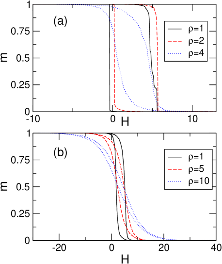
Figure 5: (Color on line) Examples of hysteresis cycles for various values of the disorder parameter $\rho$: (a) for $\rho=1,2,4$ with $\sigma=1.5$; and (b) for $\rho=1,5,10$ with $\sigma=4$. In all the cases, $\lambda=-3$, $L=16$, and $\Delta H=0.01$.

We consider the cases with $\lambda<0$ (Fig. 3(a)) and $\lambda>0$ separately (Fig. 3(b)), because they show a clearly different behavior. In the first case, which corresponds to the formation of prolate domains, the more negative $\lambda$ is, the larger the width of the loop. In the case of very negative values, the loops start to exhibit a plateau in the increasing field branch: the retransformation to the $0$ phase is done in two separate steps. (This effect will be discussed below). For the second case, increasing lambda towards positive values increases the tilt of the hysteresis loop so that saturation in the transformed phase can only be obtained when the field is very negative. This effect is due to the competition between the Potts and the dipolar terms. Many domains in the final stages of the transformation are frustrated and can only be transformed by a very negative $H$, as occurs in ferromagnets that contain a small percentage of antiferromagnetic bonds.

In Figs.  4 and 5 we show the effect of the two disorder parameters $\sigma$ (Fig. 4, in the low (a) and high (b) $\rho$ regimes) and $\rho$ (Fig. 5, in the low (a) and high (b) $\sigma$ regimes). In all the cases it can be seen that increasing the amount of disorder increases the tilt and decreases the width of the loop. Moreover, as expected, for low values of the amount of disorder ($\sigma$ or $\rho$) the loops exhibit sharp discontinuous (ferromagnetic-like) behavior. This feature is in agreement with recent results on the standard RFIM, concerning the observation that the transition from sharp to smooth loops can be induced by different kinds of disorder parameters: not only the random field variance $\sigma$ but also random anisotropy E.Vives and A.Planes (2001), the vacancy concentration X.Illa and E.Vives (2006), etc.. Our model shows that the correlation with the random fields of intensity $\rho$ can also act in a similar way.

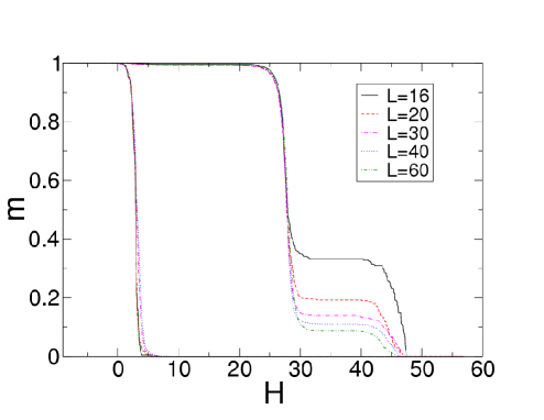
Figure 6: (Color on line) Hysteresis loop for various values of the system size $L=16,20,30,40,60$. The model parameters are: $\lambda=-25$, $\sigma=3$, $\rho=0$ and $\Delta H=0.05$

Let us now discuss the plateau observed in Fig. 3(a) in the increasing field branch. As shown in the examples in Fig. 6, this plateau occurs at smaller magnetizations when the system size is increased. This suggest that it may be due to the stabilization of “slab” domains that cross the whole system from one face to the other and that due to the periodic boundary conditions behave as infinitely large. Such slabs become less and less frequent by increasing the system size. This suggestion has been confirmed by analyzing sequences of configurations. An example will be discussed in Sec. IV.2.

In order to perform a quantitative analysis of the hysteresis loops it is important to measure some of their properties. One of the most studied hysteretic features is loop area. In fact, it represents the amount of energy dissipated during a cycle and thus it is an important quantity to be controlled both from the theoretical and materials application point of view. In Fig. 7 we show the loop area, averaged over several disorder configurations, as a function of the parameter $\lambda$, for various values of $\sigma$.

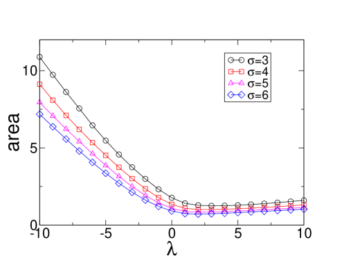
Figure 7: (Color on line) Hysteresis loop area as a function of the parameters $\lambda$, for $\sigma=3,4,5,6$. The system parameters are: $L=16$, $\Delta H=0.05$ and $\rho=0$. Each point represents an average over $800$ realizations of the disorder. Solid lines are a guide to the eye. Error bars are not visible on the scale of the picture.

As can be seen, the area shows a much more important dependence on $\lambda$ for negative than for positive $\lambda$. This behavior can also be seen by studying the coercivity (amplitude) of the hysteresis cycles at $m=0.5$, which displays a very similar dependence on $\lambda$.

In Figs. 3, 4 and 5 we can see that the hysteresis cycles obtained with our model are asymmetric, i.e. the decreasing field branch (transformation) cannot be related by an inversion operation to the increasing field branch (retransformation). This is an interesting property since, experimentally, materials displaying a transition to a multivariant phase show such behavior, which cannot be reproduced with the RFIM (see section I). In our model, this feature descends from the intrinsic difference of the physical processes occurring in the two branches (transition from the $0$ state to the three variant phase in the first branch, and the opposite process in the second branch). In order to study this feature more quantitatively, we define an asymmetry factor $A$ as:

$$A=\frac{(dM/dH)_{1}-(dM/dH)_{2}}{(dM/dH)_{1}+(dM/dH)_{2}},$$ (4)

where $(dM/dH)_{1}$ and $(dM/dH)_{2}$ are the derivatives of the hysteresis cycle at the coercive fields (defined as the two fields at a height $m=0.5$) in the two branches.

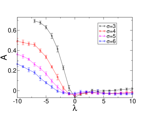
Figure 8: (Color on line) Hysteresis loop asymmetry as a function of the parameters $\lambda$, for $\sigma=3,4,5,6$. The system parameters are: : $L=16$, $\Delta H=0.05$ and $\rho=0$. Each point represents an average over $800$ realizations of the disorder. Solid lines are a guide to the eye.

As can be seen in Fig. 8, $A$ is greater than zero for negative values of $\lambda$, while for $\lambda>0$ the effect of the ’dipolar’ term is screened by the disorder and the Potts term and $A$ is essentially $0$, irrespective of the value of $\sigma$. We have cut the curve with $\sigma=3$ in Fig. 8 at the value $\lambda=-7$. In fact, for the considered range of parameter, lower $\lambda$ hysteresis curves begin to show the plateaux explained above, and thus our definition of asymmetry loses sense.

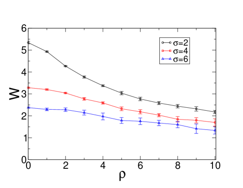
Figure 9: (Color on line) Hysteresis loop width as a function of the parameters $\rho$, for $\sigma=2,4,6$. The system parameters are: $L=16$, $\Delta H=0.05$ and $\lambda=-3$. Each point represents an average over $800$ realizations of the disorder. Solid lines are a guide to the eye.

The effect of disorder on hysteresis loop properties is illustrated in Fig. 9, where we show the width $W$ of the loops at $m=0.5$ (coercivity) as a function of increasing correlation $\rho$, for different values of $\sigma$. As mentioned in the qualitative description above, both $\rho$ and $\sigma$ decrease the width of the loops.

IV.2 Microstructures

As we have already mentioned (see section II), when the dipolar term is large enough compared to the Potts term, the transformed domains lose their spherical symmetry and start to show a non-trivial microstructure. The microstructure of a system is defined as the arrangement of the variants of the product phase.

Figure 10: (Color on line) Saturation configuration for system parameters: $L=32$, $\Delta H=0.05$, $\lambda=-72$, $\sigma=20$ and $\rho=20$. Different colors correspond to different spin variants (see the legend).

In Fig. 10 we can see an example of these three-dimensional microstructures. We represent the views of the $yz$, $xz$ and $xy$ surfaces, when the sample has reached saturation (fully transformed state). In this case ($\lambda<0$), the domains tend to be prolate. For instance green domains (corresponding to $\vec{S}_{i}=(0,0,1)$) tend to be elongated along the $z$ direction both in the $xz$ and $zy$ planes. This effect can be quantitatively measured as will be explained below.

For $\lambda>0$, we observe the formation of oblate domains, as shown in Fig. 11, developing in the plane perpendicular to the spin direction. This effect generates a sort of “chessboard” correlation as can be seen, for instance in the $yz$ plane by observing the red and green domains.

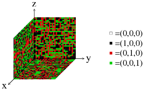
Figure 11: (Color on line) Saturation configuration for system parameters: $L=32$, $\Delta H=0.05$, $\lambda=3$, $\sigma=1$ and $\rho=1$. Different colors correspond to different spin variants (see the legend).

In order to quantify the shape of the domains in such microstructures, we have calculated the average linear size $\langle D_{x}\rangle$, $\langle D_{y}\rangle$ and $\langle D_{z}\rangle$, of the domains of the three variants $x$, $y$ and $z$, along the three spatial directions $\hat{x}$, $\hat{y}$ and $\hat{z}$, at the saturation configuration. For instance, the average size matrix corresponding to Fig. 10 and Fig. 11, are shown in Tables 1 and 2. In the first case (corresponding to the prolate domains), the diagonal elements of the matrix are sensibly larger than the others, confirming the growth tendency of domains along the orientation of each variant. As is quite obvious, for symmetry reasons, the diagonal elements can be averaged giving what we will call the average linear size in the parallel direction $\langle D_{\parallel}\rangle$ and the off-diagonal elements can also be averaged giving the average linear size in the perpendicular direction $\langle D_{\perp}\rangle$. For the case of Fig. 10 ($\lambda<0$) we get $\langle D_{\parallel}\rangle=4.44\pm 0.20$ and $\langle D_{\perp}\rangle=2.19\pm 0.05$. For the case of Fig. 11 ($\lambda>0$), the tendency of the system to form oblate domains is confirmed by the values $\langle D_{\parallel}\rangle=1.175\pm 0.005$ and $\langle D_{\perp}\rangle=1.89\pm 0.03$.

	$\langle D_{x}\rangle$	$\langle D_{y}\rangle$	$\langle D_{z}\rangle$
$\hat{x}$	4.35 $\pm$ 0.14	2.21 $\pm$ 0.02	2.20 $\pm$ 0.02
$\hat{y}$	2.04 $\pm$ 0.02	4.22 $\pm$ 0.13	2.15 $\pm$ 0.02
$\hat{z}$	2.27 $\pm$ 0.02	2.28 $\pm$ 0.02	4.75 $\pm$ 0.07

Table 1: Average size matrix for the saturation configuration of Fig. 10.

	$\langle D_{x}\rangle$	$\langle D_{y}\rangle$	$\langle D_{z}\rangle$
$\hat{x}$	1.172 $\pm$ 0.003	1.927 $\pm$ 0.014	1.903 $\pm$ 0.014
$\hat{y}$	1.862 $\pm$ 0.013	1.173 $\pm$ 0.003	1.868 $\pm$ 0.013
$\hat{z}$	1.876 $\pm$ 0.013	1.887 $\pm$ 0.013	1.181 $\pm$ 0.003

Table 2: Average size matrix for the saturation configuration of Fig. 11.

For the sake of completeness, as a final microstructure example, in Fig. 12 we show a system configuration with high disorder and $\lambda=0$. As expected, no domain asymmetry arises and every spin just aligns with its local random field. The values of $\langle D_{\parallel}\rangle=1.51\pm 0.14$ and $\langle D_{\perp}\rangle=1.50\pm 0.20$ are equal to within statistical errors.

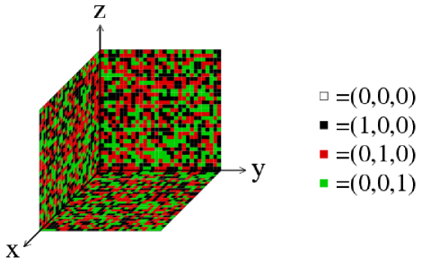
Figure 12: (Color on line) Saturation configuration for system parameters: $L=32$, $\Delta H=0.05$, $\lambda=0$, $\sigma=40$ and $\rho=40$. Different colors correspond to different spin variants (see the legend).

	$\langle D_{x}\rangle$	$\langle D_{y}\rangle$	$\langle D_{z}\rangle$
$\hat{x}$	1.509 $\pm$ 0.082	1.491 $\pm$ 0.080	1.492 $\pm$ 0.079
$\hat{y}$	1.517 $\pm$ 0.083	1.511 $\pm$ 0.081	1.504 $\pm$ 0.080
$\hat{z}$	1.512 $\pm$ 0.082	1.512 $\pm$ 0.082	1.515 $\pm$ 0.081

Table 3: Average size matrix for the saturation configuration of Fig. 12.

The formation of microstructures such as those in Fig. 10 and 11 is quite clearly affected by the dynamics due to the effect of kinetic constraints. In fact, when a domain of one variant starts to grow, it necessarily blocks the growth of neighboring domains of other variants and vice versa. Thus the first variant to locally break symmetry will facilitate the nucleation of large domains, thus restricting the dimensions of the other variants. This effect could be seen, for instance, by analyzing the decreasing field branch in Fig. 13: the formation of the domains of type $x$ and $y$ that cross the system block the growth of domains of the $z$ variant.

Moreover, with the help of the microstructure representation, we can analyze in more detail the bump formation due to finite size effects, discussed in section IV.1 (see Fig. 13): in fact, if the system size is finite there is the formation of domains spanning a whole system side, such as the $y$ domains in microstructures labeled with $4$ and $5$ in Fig. 13. As already pointed out, these kind of slab domains are actually infinite due to the periodic boundary conditions and are thus very stable. As we can see in the figure, they keep existing up to high driving field, giving rise to the existence of the plateau and disappear when the field overcomes a certain threshold.

Figure 13: (Color on line) Parameters: $L=32$, $\lambda=-12$, $\sigma=1.5$, $\Delta H=0.05$ and $\rho=0$. The configuration snapshots are taken for (1) $m=0.03$; (2) $m=0.98$; (3) $m=1$; (4) $m=0.78$; (5) $m=0.28$ and (6) $m=0.18$.

As we already mentioned in section II, the truncation of the dipolar term does not allow elastic effects to be reproduced, which would lead to more realistic microstructure. In particular, it would be interesting to control the tendency for the different variants to exhibit a preferred habit plane, as would be the case of a real cubic to tetragonal transition. We expect that including a next-nearest-neighbor dipolar interaction will allow for such an interesting property to occur. The model presented here is, therefore, a promising starting point for modeling materials with a phase transition from a single variant to a multivariant phase.

IV.3 Avalanches

Another phenomenon that may be analyzed with our model is the avalanche dynamics. The hysteresis loops in athermal first-order phase transitions consist of a sequence of jumps between metastable states. Such discontinuities are, in general, microscopic. However, for certain values of the disorder one or more may become comparable to the system size and then correspond to the observed macroscopic discontinuities in the ferromagnetic loops. In the magnetic case, microscopic avalanches can be detected experimentally by appropriate coils. They correspond to the so-called Barkhausen noise H.Barkhausen (1919). In structural transitions, avalanches can also be detected typically by acoustic emission techniques Vives et al. (1994). Knowledge of the distribution of the number of avalanches along the transition, as well as their size and duration, is an important piece of information in order to characterize athermal FOPT.

Good discrimination of individual avalanches in the simulations can only be performed in the limit of $\Delta H\rightarrow 0$. This will require a true adiabatic simulation algorithm which is not available at present, as opposed to the case of the standard RFIM Kuntz et al. (1999). In our case, after a small (but finite) change $\Delta H$ some spins can be updated. We will consider all of them as being part of a single avalanche. This is an approximation and, therefore, we should keep in mind the fact that we are slightly overestimating the size of the observed avalanches due to some unavoidable overlaps. In the experiments recording avalanches the same problem occurs R.A.White and K.A.Dahmen (2003); Pérez-Reche et al. (2004).

With this definition we can study, for instance, the average number of avalanches $\langle N_{av}\rangle$ as a function of the external field $H$. As an example, in Fig. 14(a) we present the behavior of this number for the case $\lambda=-8$, $\sigma=4$, $\rho=0$, compared with the behavior of the average hysteresis loop in Fig. 14 (b). $\langle N_{av}\rangle$ presents two peaks in correspondence with the two coercive fields and goes to zero (as expected) at the $m=0$ and $m=1$ saturations. This kind of information is very relevant for the understanding of the measurements of acoustic emission in structural transitions using the pulse-counting technique F.J.Pérez-Reche et al. (2004).

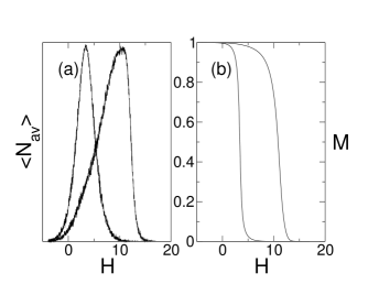
Figure 14: (a) Number of avalanches $N_{av}$ (arbitrary units) as a function of the external field. $N_{av}$ is computed in each $\Delta H$ interval over $600$ loops, and (b): The related averaged hysteresis cycle. Simulation parameters: $L=16$, $\Delta H=0.02$, $\lambda=-8$, $\sigma=4$, $\rho=0$.

More interesting information can be obtained by measuring the avalanche sizes $S$ and computing the integrated probability distribution $P(S)$, by analyzing all the avalanches in a single branch of the loop (the two branches must be analyzed separately since they are not symmetric). As a naive approximation, in our case one can define in our case the size $S$ of the avalanche as the order parameter variation $\Delta M$ associated with an avalanche (i.e. when the field is varied by $\Delta H$.) Nevertheless, this definition imported from the standard RFIM should be carefully adapted to our multivariant FOPT. Inside an avalanche, in fact, one can distinguish between different kinds of processes taking place, depending on their effect on the order parameter variation. Let us focus on the decreasing field branch starting from the $m=0$ phase up to the $m=1$ saturated configuration: there are several microscopic possibilities for a spin jump. A spin could jump from the $0$ state to one of the three variants $x$, $y$ and $z$ thus giving rise to a positive contribution to the magnetization change $\Delta M$; it could jump from the $x$, $y$ or $z$ states to $0$, causing a negative contribution $\Delta M<0$; or finally there is a possibility of a change from one variant to another without contributing to the change in the system magnetization. These three possible updates will be called $+$, $-$ and $0$. Instead of only measuring the total size $\Delta M$ of an avalanche, for each of them we will measure the three quantities $n_{+}$, $n_{-}$ and $n_{0}$, which are the number of spin updates of each kind. Moreover, since as we have seen in section IV.1, the hysteresis loops are not symmetric, we should separately analyze the avalanches during the decreasing field branch and during the increasing field branch. This gives, therefore, 6 possible distributions: $P_{+}^{down}(n)$, $P_{-}^{down}(n)$, $P_{0}^{down}(n)$ for the decreasing field branch and $P_{+}^{up}(n)$, $P_{-}^{up}(n)$, $P_{0}^{up}(n)$ for the increasing field branch. It should be mentioned that in the increasing field branch the total number of events of the $+$ and $0$ kind are much smaller than the number of $-$ events, typically by 2-3 orders of magnitude. For the decreasing branch the $-$ events are rare, but $0$ events are frequent, since an important number of transitions within variants may occur during the avalanches in the later stages of the transition. Of course such an optimization between variants cannot occur in the reverse process during the increasing field branch.

In Figs. 15 and 16 we show some examples of the probability distributions for varying values of the two disorder parameters on log-log plots, respectively $\sigma$ and $\rho$. Actually, we show only the $P_{+}^{down}(n)$ and the $P_{-}^{up}(n)$ distributions which account for the majority of the events. In Fig. 15(b) it is possible to notice another finite size effect: the slab domains of size corresponding to multiples of the system size $L$ present the tendency to disappear abruptly (and thus the $P^{-}_{up}(n)$ presents some peaks in correspondence of values multiple of $L$), as we have already pointed out in section IV.2.

An interesting result for the case of $\rho=0$ (see Fig. 15(a)) is that the distribution $P_{+}^{down}(n)$ shows a exponentially damped behavior but seems to become a power-law for a certain critical value of $\sigma$ (which will be located around $\sigma\simeq 3$). Such a tendency has been well studied in the standard RFIM. The fitted value of the power-law exponent is 1.1, clearly smaller than the expected universal value $2.03\pm 0.03$ Perković et al. (1999), but this feature could be due to finite size effect. Only a detailed finite-size scaling analysis and the study of the geometry of the avalanches F.J.Pérez-Reche and E.Vives (2003) (out of the scope of this paper) will reveal if the observed power law conforms to universal behavior or not. Interestingly it seems that for the increasing field branch (see Fig. 15(b)), the distribution is always exponentially damped, at least for the studied range of values of $\sigma$. Therefore, the critical point for the increasing field branch, if it exists, would be located at a different (smaller) value of $\sigma$.

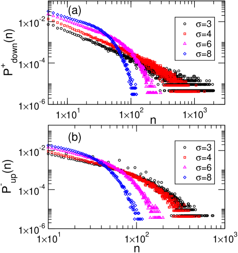
Figure 15: (Color on line) Avalanche size probability distributions $P_{+}^{down}(n)$ (a) and $P_{-}^{up}(n)$ (b) corresponding to the two branches of the hysteresis loop, averaged over $600$ disorder realizations and for four values of $\sigma$ as indicated by the legend. Simulation parameters are : $L=16$, $\Delta H=0.05$, $\lambda=-8$ and $\rho=0$.

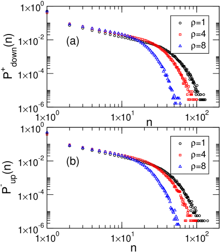
Figure 16: (Color online) Avalanche size probability distributions $P_{+}^{down}(n)$ and $P_{-}^{up}(n)$ corresponding to the two branches of the hysteresis loop, averaged over $600$ disorder realizations and for three valued of $\rho$. Simulation parameters are: $L=16$, $\Delta H=0.05$, $\lambda=-8$ and $\sigma=8$.

V Summary

The analysis of microstructure formation in ferroic systems undergoing a first-order phase transitions is an interesting issue both from a purely theoretical and an applicative point of view. Microstructures arise since the product phase, arising from the balance of many energetic terms, may show energetically equivalent variants. Despite the interest in this issue, the models that have been used up to now for the study of the interplay between disorder and athermal evolution (for example, the Random Field Ising model Sethna et al. (1993)) are not suitable for the analysis of microstructure formation, due to the equivalence of the variants of the product phase.

In the present work, we have introduced a modification of the Random Field Potts model, which consists of adding a dipolar term truncated to the nearest-neighbor approximation, which represents a promising step towards the analysis of athermal transitions from a degenerate to a multivariant phase.

In our simulations we have chosen extremal updating in order to preserve the independence of the trajectory from the applied field rate. We have studied the dependence of the hysteresis loop shape on the hamiltonian parameters values. From a quantitative point of view, this has been performed by measuring the the loop area, its asymmetry and width. Our loops display a large area and asymmetry regime for very negative values of the ’dipolar’ term parameter $\lambda$, associated with the formation of microstructures with prolate domains, oriented along three equivalent spatial directions. On the other hand, for $\lambda>0$ domains are planar (oblate) and the loops show low, almost constant values of the area and the asymmetry.

We have also addressed the study of the avalanches in the hysteresis loop, distinguishing between the two branches. For certain parameter values, the probability distribution of the size of the leading process in an avalanche displays power-law behavior, which is the typical result for athermal phase transitions in disordered systems.