The Form of the Effective Interaction in Harmonic-Oscillator-Based Effective Theory

Abstract

I explore the form of the effective interaction in harmonic-oscillator-based effective theory (HOBET) in leading-order (LO) through next-to-next-to-next-to-leading order (N³LO). As the included space in a HOBET (as in the shell model) is defined by the oscillator energy, both long-distance (low-momentum) and short-distance (high-momentum) degrees of freedom reside in the high-energy excluded space. A HOBET effective interaction is developed in which a short-range contact-gradient expansion, free of operator mixing and corresponding to a systematic expansion in nodal quantum numbers, is combined with an exact summation of the relative kinetic energy. By this means the very strong coupling of the included ($P$) and excluded ($Q$) spaces by the kinetic energy is removed. One finds a simple and rather surprising result, that the interplay of $QT$ and $QV$ is governed by a single parameter $\kappa$, the ratio of an observable, the binding energy $|E|$, to a parameter in the effective theory, the oscillator energy $\hbar\omega$. Once the functional dependence on $\kappa$ is identified, the remaining order-by-order subtraction of the short-range physics residing in $Q$ becomes systematic and rapidly converging. Numerical calculations are used to demonstrate how well the resulting expansion reproduces the running of $H^{eff}$ from high scales to a typical shell-model scale of 8$\hbar\omega$. At N³LO various global properties of $H^{eff}$ are reproduced to a typical accuracy of 0.01%, or about 1 keV, at 8$\hbar\omega$. Channel-by-channel variations in convergence rates are similar to those found in effective field theory approaches.

The state-dependence of the effective interaction has been a troubling problem in nuclear physics, and is embodied in the energy dependence of $H^{eff}(|E|)$ in the Bloch-Horowitz formalism. It is shown that almost all of this state dependence is also extracted in the procedures followed here, isolated in the analytic dependence of $H^{eff}$ on $\kappa$. Thus there exists a simple, Hermitian $H^{eff}$ that can be use in spectral calculations.

The existence of a systematic operator expansion for $H^{eff}$, depending on a series of short-range constants augmented by $\kappa$, will be important to future efforts to determine the HOBET interaction directly from experiment, rather than from an underlying NN potential.

I Introduction

In nuclear physics one often faces the problem of determining long-wavelength properties of nuclei, such as binding energies, radii, or responses to low-momentum probes. One approach would be to evaluate the relevant operators between exact nuclear wave functions obtained from solutions of the many-body Schroedinger equation. Because the NN potential is strong, characterized by anomalously large NN scattering lengths, and highly repulsive at very short distances, this task becomes exponentially more difficult as the nucleon number increases. Among available quasi-exact methods, the variational and Green’s function Monte Carlo work of the Argonne group has perhaps set the standard argonne , yielding accurate results throughout most of the $1p$ shell.

Effective theory (ET) potentially offers an alternative, a method that limits the numerical difficulty of a calculation by restricting it to a finite Hilbert space (the $P$- or “included”-space), while correcting the bare Hamiltonian $H$ (and other operators) for the effects of the $Q$- or “excluded”-space. Calculations using the effective Hamiltonian $H^{eff}$ within $P$ reproduce the results using $H$ within $P+Q$, over the domain of overlap. That is, the effects of $Q$ on $P$-space calculations are absorbed into $P(H^{eff}-H)P$.

One interesting challenge for ET is the case of a $P$-space basis of harmonic oscillator (HO) Slater determinants. This is a special basis for nuclear physics because of center-of-mass separability: if all Slater determinants containing up to $N$ oscillator quanta are retained, $H^{eff}$ will be translationally invariant (assuming $H$ is). Such bases are also important because of powerful shell-model (SM) techniques that have been developed for iterative diagonalization and for evaluating inclusive responses. The larger $P$ can be made, the smaller the effects of $H^{eff}-H$. If one could fully develop harmonic-oscillator based effective theory (HOBET), it would provide a prescription for eliminating the SM’s many uncontrolled approximations, while retaining the model’s formidable numerical apparatus.

The long-term goal is a HOBET resembling standard effective field theories (EFTs) weinberg ; savage . That is, for a given choice of $P$, the effective interaction would be a sum of a long-distance “bare” interaction whose form would be determined by chiral symmetry, augmented by some general effective interaction that accounts for the excluded Q space. That effective interaction would be expanded systematically and in some natural way, with the parameters governing the strength of successive terms determined by directly fitting to experiment. There would be no need to introduce or integrate out any high-momentum NN potential, an unnecessary intermediate effective theory between QCD and the SM scale.

One prerequisite for such an approach is the demonstration that a systematic expansion for the HOBET effective interaction exists. This paper explores this issue, making use of numerically generated effective interaction matrix elements for the deuteron, obtained by solving the Bloch-Horowitz (BH) equation for the Argonne $v_{18}$ potential, an example of a potential with a relatively hard core ($\mathrel{\hbox to0.0pt{\lower 4.0pt\hbox{\hskip 1.0pt$\sim$}\hss}\raise 1.0pt\hbox{$<$}}$ 2 GeV) av18 . The BH $H^{eff}$ is a Hermitian but energy-dependent Hamiltonian satisfying

$$H^{eff}=H + H{1\over E-QH}QH$$

$$H^{eff}|\Psi_{P}\rangle=E|\Psi_{P}\rangle~{}~{}~{} ~{}~{}~{}|\Psi_{P}\rangle=(1-Q)|\Psi\rangle.$$ (1)

Here $H$ is the bare Hamiltonian and $E$ and $\Psi$ are the exact eigenvalue and wave function (that is, the solution of the Schroedinger equation in the full $P+Q$ space). $E$ is negative for a bound state. Because $H^{eff}$ depends on the unknown exact eigenvalue $E$, Eqs. (1) must be solved self-consistently, state by state, a task that in practice proves to be relatively straightforward. If this is done, the $P$-space eigenvalue will be the exact energy $E$ and the $P$-space wave function $\Psi_{P}$ will be the restriction of the exact wave function $\Psi$ to $P$. This implies a nontrivial normalization and nonorthogonality of the restricted ($P$-space) wave functions. If $P$ is enlarged, new components are added to the existing ones, and for a sufficiently large $P$ space, the norm approaches ones. This convergence is slow for potentials like $v_{18}$, with many shells being required before norms near one are achieved song ; luu . Observables calculated with the restricted wave functions and the appropriate effective operators are independent of the choice of $P$, of course. All of these properties follow from physics encoded in $H^{eff}$.

In HOBET $P$ and thus $H^{eff}$ are functions of the oscillator parameter $b$ and the number of included HO quanta $\Lambda_{P}$. In this paper I study the behavior of matrix elements $\langle\alpha|H^{eff}|\beta\rangle$ generated for the Argonne $v_{18}$ potential, as both $b$ and $\Lambda_{P}$ are varied. In particular, $\Lambda_{P}$ is allowed to run from very high values to the “shell-model” scale of 8 $\hbar\omega$, in order to test whether the physics above a specified scale can be efficiently absorbed into the coefficients of some systematic expansion, e.g., one analogous to the contact-gradient expansions employed in EFTs (which are generally formulated in plane wave bases). There are reasons the HOBET effective interaction could prove more complicated:

• An effective theory defined by a subset of HO Slater determinants is effectively an expansion around a typical momentum scale $q\sim 1/b$. That is, the $P$-space omits both long-wavelength and short-wavelength degrees of freedom. The former are connected with the overbinding of the HO, while the latter are due to absence in $P$ of the strong, short-range NN interaction. As any systematic expansion of the effective interaction must simultaneously address both problems, the form of the effective interaction cannot be as simple as a contact-gradient expansion (which would be appropriate if the missing physics were only short-ranged).

• The relative importance of the missing long-wavelength and short-wavelength excitations is governed by the binding energy, $|E|$, with the former increasing as $|E|\rightarrow 0$. These long-range interactions allow nuclear states to de-localize, minimizing the kinetic energy. But nuclei are weakly bound – binding energies are very small compared to the natural scales set by the scalar and vector potentials in nuclei. One concludes that the effective interaction must depend delicately on $|E|$.

• An effective theory is generally considered successful if it can reproduce the lowest energy excitations in $P$. But one asks for much more when one seeks to accurately represent the effective interaction, which governs all of the spectral properties within $P$. The HO appears to be an especially difficult case in which to attempt such a representation. The kinetic energy operator in the HO has strong off-diagonal components which raise or lower the nodal quantum number, and thus connect Slater determinants containing $\Lambda_{P}$ quanta with those containing $\Lambda_{P}\pm 2$. This means that $P$ and $Q$ are strongly coupled through low-energy excitations, a situation that is usually problematic for an effective theory.

All of these problems involve the interplay, governed by $|E|$, of $QT$ (delocalization) and $QV$ (corrections for short-range repulsion). The explicit energy dependence of the BH equation proves to be a great advantage in resolving the problems induced by this interplay, leading to a natural factorization of the long- and short-range contributions to the effective interaction, and thereby to a successful systematic representation of the effective interaction. (Conversely, techniques such as Lee-Suzuki suzuki will intermingle these effects in a complex way and obscure the underlying simplicity of the effective interaction.) The result is an energy-dependent contact-gradient expansion at N³LO that reproduces the entire effective interaction to an accuracy of about a few keV. The contact-gradient expansion is defined in a way that is appropriate to the HO, eliminating operator mixing and producing a simple dependence on nodal quantum numbers. The coefficients in the expansion play the role of generalized Talmi integrals.

The long-range physics residing in $Q$ can be isolated analytically and expressed in terms of a single parameter, $\kappa=\sqrt{2|E|/\hbar\omega}$, remarkably the ratio of an observable ($|E|$) to a parameter one chooses in defining the ET. The dependence of $H^{eff}$ on $\kappa$ is determined by summing $QT$ to all orders. The resulting $H^{eff}$ is defined by $\kappa$ and by the coefficients of the short-ranged expansion.

This same parameter governs almost all of the state dependence that enters when one seeks to describe multiple states. Thus it appears that there is a systematic, rapidly converging representation for $H^{eff}$ in HOBET that could be used to describe a set of nuclear states. The short-range parameters in that representation are effectively state-independent, as the state-dependence usually attacked with techniques like Lee-Suzuki is isolated in $\kappa$.

II Long- and short-wavelength separations in $H^{eff}$

In Refs. song ; luu a study was done of the evolution of matrix elements $\langle\alpha|H^{eff}|\beta\rangle$, for the deuteron and for ³He/³H, from the $\Lambda_{P}\rightarrow\infty$ limit, where $H^{eff}\rightarrow H$, down to $\Lambda_{P}$ characteristic of the shell model (SM), e.g., small $P$ spaces with 4, 6, or 8 $\hbar\omega$ excitations, relative to the naive $1s$-shell ground state. As noted above, this definition of $P$ in terms of the total quanta in HO Slater determinants maintains center-of-mass separability and thus leads to an $H^{eff}$ that is translationally invariant, just like $H$. Indeed, the HO basis is the only set of compact wave functions with this attractive property.

But this choice leads to a more complicated ET, as $P$ excludes both short-distance and long-distance components of wave functions. This problem was first explored in connection with the nonperturbative behavior of $H^{eff}$: the need to simultaneously correct for the missing long- and short-distance behavior of $\Psi_{P}$ is the reason one cannot tune $P$ to make $H^{eff}$ converge rapidly. For example, while it is possible to “pull” more of the missing short-range physics into $P$ by choosing a small $b$, this adjustment produces a more compact state with very large $Q$-space corrections to the kinetic energy. Conversely, one can tune $b$ to large values to improve the description of the nuclear tail, but at the cost of missing even more of the short-range physics. At no value of $b$ are both problems handled well: Fig. 1 shows that a poor minimum is reached at some intermediate $b$, with a $10\hbar\omega$ “bare” calculation failing to bind the deuteron.

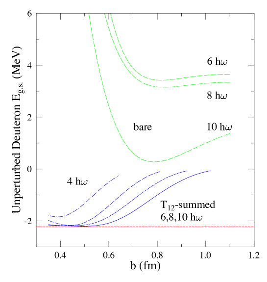
Figure 1: (Color online) Deuteron ground-state convergence for “bare” calculations in small $P$-spaces, which omit all effects due to the multiple scattering of $V$ in $Q$. The three curves on the upper right were calculated from the standard BH equation, which identifies the bare interaction as $P(T+V)P$. These calculations fail to bind the deuteron, even with $\Lambda_{P}=10$, for all values of the HO size parameter $b$: the $P$-space estimate for $V$ is poor if $b$ is much above 1fm, while the estimate for $T$ is poor if $b$ is below that value. The lower four curves were evaluated for the bare interaction of the reordered BH given by Eq. (2), which incorporates the long-range effects of $QT$ to all orders, building in the correct asymptotic form of the wave function. This allows one to reduce $b$ to small values, pulling most of the effects of $V$ into $P$, without distorting the long-distance behavior of the wave function or, therefore, the estimate for $T$. Rather remarkably, this bare calculation reproduces the correct binding energy for $P$ spaces as small as $\Lambda_{P}$=6. That is, by the combination of the summation of $QT$ to all orders and the adjustment of $b$ to an optimal value characteristic of the hard core radius of $v_{18}$, the effective interaction contribution can be driven to such small values that it can be ignored.

The solution found to this hard-core correlation/extended state quandary is an a priori treatment of the overbinding of the harmonic oscillator. The BH equation is rewritten in a form that allows the relative kinetic energy operator to be summed to all orders. (This form was introduced in the first of Refs. luu ; a detailed derivation can be found in the Appendix of the third of these references. The kinetic energy sum can be done analytically for calculations performed in a Jacobi basis.) This reordered BH equation has the form

$$H^{eff}=H+HQ{1\over E-QH}QH={E\over E-TQ}\left[T-T{Q\over E}T+V+V{1\over E-QH}QV\right]{E\over E-QT}$$ (2)

where the bare $H$ is the sum of the relative kinetic energy and a two-body interaction

$$H={1\over 2}\sum_{i,j=1}^{A}\left(T_{ij}+V_{ij}\right),\mathrm{~{}~{}~{}with~{}~{}}T_{ij}={({\bf p}_{i}-{\bf p}_{j})^{2}\over 2AM}.$$ (3)

This effective interaction is to be evaluated between a finite basis of Slater determinants $|\alpha\rangle\in P$, which is equivalent to evaluating the Hamiltonian

$$\widetilde{H}^{eff}\equiv T-T{Q\over E}T+V+V{1\over E-QH}QV$$ (4)

between the states

$$|\widetilde{\alpha}\rangle\equiv{E\over E-QT}|\alpha\rangle$$ (5)

By summing $QT$ to all orders, the proper behavior at large $r$ can be built in, which then allows $b$ to be adjusted, without affecting the long-wavelength properties of the wave function. Fig. 1, from Ref. luu , shows that the resulting decoupling of the long- and short-wavelength physics can greatly improve convergence: a “bare” 6 $\hbar\omega$ calculation that neglects all contributions of $QV$ gives an excellent binding energy. This decoupling of $QV$ and $QT$ is also important in finding a systematic expansion for $H^{eff}$.

This reorganization produces an $H^{eff}$ with three terms operating between HO Slater determinants,

$$\langle\alpha|T{E\over E-QT}|\beta\rangle=\langle\alpha|{E\over E-TQ}T|\beta\rangle~{} \stackrel{{\scriptstyle\mathrm{nonedge}}}{{\longrightarrow}} ~{}\langle\alpha|T|\beta\rangle$$

$$\langle\alpha|{E\over E-TQ}V{E\over E-QT}|\beta\rangle~{} \stackrel{{\scriptstyle\mathrm{nonedge}}}{{\longrightarrow}} ~{}\langle\alpha|V|\beta\rangle$$

$$\langle\alpha|{E\over E-TQ}V{1\over E-QH}QV{E\over E-QT}|\beta\rangle~{} \stackrel{{\scriptstyle\mathrm{nonedge}}}{{\longrightarrow}} ~{}\langle\alpha|V{1\over E-QH}QV|\beta\rangle.$$ (6)

The ladder properties of $QT$ make $E/(E-QT)$ the identity operator except when it acts on an $|\alpha\rangle$ with energy $\Lambda_{P}\hbar\omega$ or $(\Lambda_{P}-1)\hbar\omega$. These are called the edge states. For nonedge states, the new grouping of terms in $H^{eff}$ reduces to the expressions on the right-hand side of Eq. 6, the conventional components of $H^{eff}$. Thus the summation over $QT$ alters only a subset of the matrix elements of $H^{eff}$, while leaving other states unaffected.

Figure 2 shows the extended tail of the relative two-particle wave function that is induced by $E/(E-QT)$ acting on an edge HO state luu . As will become apparent from later expressions, this tail has the proper exponential fall-off,

$$\sim{e^{-\kappa r}\over\kappa r}$$ (7)

where $\kappa=\sqrt{2|E|/\hbar\omega}$ and $r=|\vec{r}_{1}-\vec{r}_{2}|/\sqrt{2}b$ is the dimensionless Jacobi coordinate, not the Gaussian tail of the HO. At small $r$ the wave function is basically unchanged (apart from normalization).

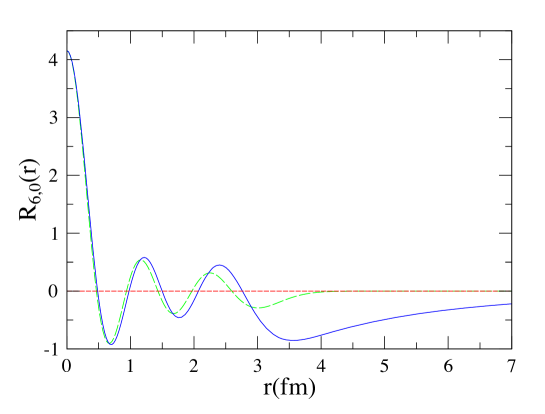
Figure 2: (Color online) A comparison of the radial wave functions for the HO state $|nl\rangle$ (dashed) and for the extended state $(E/E-QT)|nl\rangle$ (solid), for $(n,l)=(6,0)$ in a $\Lambda_{P}=10$ deuteron calculation. The extended tail of the latter is apparent. Note that the normalization of the extended state has been adjusted to match that of $|nl\rangle$ at $r$=0, in order to show that the shapes differ only at large $r$. Thus a depletion of the extended state at small $r$ is not apparent in this figure.

III The HOBET Effective Interaction

Contact-gradient expansions are used in approaches like EFT to correct for the exclusion of short-range (high-momentum) interactions. The most general scalar interaction is constructed, consistent with Hermiticity, parity conservation, and time-reversal invariance, as an expansion in the momentum. Such an interaction for the two-nucleon system, expanded to order N³LO (or up to six gradients), is shown in Table 1. (Later these operators will be slightly modified for HOBET.)

Table 1: Contact-gradient expansion for relative-coordinate two-particle matrix elements. Here $\stackrel{{\scriptstyle\rightarrow}}{{D^{2}_{M}}}=(\stackrel{{\scriptstyle\rightarrow}}{{\nabla}}\otimes\stackrel{{\scriptstyle\rightarrow}}{{\nabla}})_{2M}$, $\stackrel{{\scriptstyle\rightarrow}}{{D^{0}_{0}}}=[(\sigma(1)\otimes\sigma(2))_{2}\otimes D^{2}]_{00}$, $\stackrel{{\scriptstyle\rightarrow}}{{F^{3}_{M}}}=(\stackrel{{\scriptstyle\rightarrow}}{{\nabla}}\otimes\stackrel{{\scriptstyle\rightarrow}}{{D^{2}}})_{3M}$, $\stackrel{{\scriptstyle\rightarrow}}{{F^{1}_{M}}}=[(\sigma(1)\otimes\sigma(2))_{2}\otimes F^{3}]_{1M}$, $\stackrel{{\scriptstyle\rightarrow}}{{G^{4}_{M}}}=(\stackrel{{\scriptstyle\rightarrow}}{{D^{2}}}\otimes\stackrel{{\scriptstyle\rightarrow}}{{D^{2}}})_{4M},$ $\stackrel{{\scriptstyle\rightarrow}}{{G^{2}_{M}}}=[(\sigma(1)\otimes\sigma(2))_{2}\otimes G^{4}]_{2M}$, and the scalar product of tensor operators is defined as $A^{J}\cdot B^{J}=\sum_{M=-J}^{M=J}(-1)^{M}A^{J}_{M}B^{J}_{-M}$.

Transitions	LO	NLO	NNLO	N3LO
${}^{3}S_{1}\leftrightarrow{}^{3}S_{1}$	$a_{LO}^{3S1}\delta({\bf r})$	$a_{NLO}^{3S1}(\stackrel{{\scriptstyle\leftarrow}}{{\nabla^{2}}}\delta({\bf r})+\delta({\bf r})\stackrel{{\scriptstyle\rightarrow}}{{\nabla^{2}}})$	$a_{NNLO}^{3S1,22}\stackrel{{\scriptstyle\leftarrow}}{{\nabla^{2}}}\delta({\bf r})\stackrel{{\scriptstyle\rightarrow}}{{\nabla^{2}}}$	$a_{N^{3}LO}^{3S1,42}(\stackrel{{\scriptstyle\leftarrow}}{{\nabla^{4}}}\delta({\bf r})\stackrel{{\scriptstyle\rightarrow}}{{\nabla^{2}}}+\stackrel{{\scriptstyle\leftarrow}}{{\nabla^{2}}}\delta({\bf r})\stackrel{{\scriptstyle\rightarrow}}{{\nabla^{4}}})$
or ${}^{1}S_{0}\leftrightarrow{}^{1}S_{0}$			$a_{NNLO}^{3S1,40}(\stackrel{{\scriptstyle\leftarrow}}{{\nabla^{4}}}\delta({\bf r})+\delta({\bf r})\stackrel{{\scriptstyle\rightarrow}}{{\nabla^{4}}})$	$a_{N^{3}LO}^{3S1,60}(\stackrel{{\scriptstyle\leftarrow}}{{\nabla^{6}}}\delta({\bf r})+\delta({\bf r})\stackrel{{\scriptstyle\rightarrow}}{{\nabla^{6}}}$)
${}^{3}S_{1}\leftrightarrow{}^{3}D_{1}$		$a_{NLO}^{SD}(\delta({\bf r})\stackrel{{\scriptstyle\rightarrow}}{{D^{0}}}+\stackrel{{\scriptstyle\leftarrow}}{{D^{0}}}\delta({\bf r}))$	$a_{NNLO}^{SD,22}(\stackrel{{\scriptstyle\leftarrow}}{{\nabla^{2}}}\delta({\bf r})\stackrel{{\scriptstyle\rightarrow}}{{D^{0}}}+\stackrel{{\scriptstyle\leftarrow}}{{D^{0}}}\delta({\bf r})\stackrel{{\scriptstyle\rightarrow}}{{\nabla^{2}}})$	$a_{N^{3}LO}^{SD,42}(\stackrel{{\scriptstyle\leftarrow}}{{\nabla^{4}}}\delta({\bf r})\stackrel{{\scriptstyle\rightarrow}}{{D^{0}}}+\stackrel{{\scriptstyle\leftarrow}}{{D^{0}}}\delta({\bf r})\stackrel{{\scriptstyle\rightarrow}}{{\nabla^{4}}})$
			$a_{NNLO}^{SD,04}(\delta({\bf r})\stackrel{{\scriptstyle\rightarrow}}{{\nabla^{2}}}\stackrel{{\scriptstyle\rightarrow}}{{D^{0}}}+\stackrel{{\scriptstyle\leftarrow}}{{D^{0}}}\stackrel{{\scriptstyle\leftarrow}}{{\nabla^{2}}}\delta({\bf r}))$	$a_{N^{3}LO}^{SD,24}(\stackrel{{\scriptstyle\leftarrow}}{{\nabla^{2}}}\delta({\bf r})\stackrel{{\scriptstyle\rightarrow}}{{\nabla^{2}}}\stackrel{{\scriptstyle\rightarrow}}{{D^{0}}}+\stackrel{{\scriptstyle\leftarrow}}{{D^{0}}}\stackrel{{\scriptstyle\leftarrow}}{{\nabla^{2}}}\delta({\bf r})\stackrel{{\scriptstyle\rightarrow}}{{\nabla^{2}}})$
				$a_{N^{3}LO}^{SD,06}(\delta({\bf r})\stackrel{{\scriptstyle\rightarrow}}{{\nabla^{4}}}\stackrel{{\scriptstyle\rightarrow}}{{D^{0}}}+\stackrel{{\scriptstyle\leftarrow}}{{D^{0}}}\stackrel{{\scriptstyle\leftarrow}}{{\nabla^{4}}}\delta({\bf r}))$
${}^{1}D_{2}\leftrightarrow{}^{1}D_{2}$			$a_{NNLO}^{1D2}\stackrel{{\scriptstyle\leftarrow}}{{D^{2}}}\cdot\delta({\bf r})\stackrel{{\scriptstyle\rightarrow}}{{D^{2}}}$	$a_{N^{3}LO}^{1D2}(\stackrel{{\scriptstyle\leftarrow}}{{D^{2}}}\stackrel{{\scriptstyle\leftarrow}}{{\nabla^{2}}}\cdot\delta({\bf r})\stackrel{{\scriptstyle\rightarrow}}{{D^{2}}}+\stackrel{{\scriptstyle\leftarrow}}{{D^{2}}}\cdot\delta({\bf r})\stackrel{{\scriptstyle\rightarrow}}{{\nabla^{2}}}\stackrel{{\scriptstyle\rightarrow}}{{D^{2}}})$
or ${}^{3}D_{J}\leftrightarrow{}^{3}D_{J}$
${}^{3}D_{3}\leftrightarrow{}^{3}G_{3}$				$a_{N^{3}LO}^{DG}(\stackrel{{\scriptstyle\leftarrow}}{{D^{2}}}\cdot\delta({\bf r})\stackrel{{\scriptstyle\rightarrow}}{{G^{2}}}+\stackrel{{\scriptstyle\leftarrow}}{{G^{2}}}\cdot\delta({\bf r})\stackrel{{\scriptstyle\rightarrow}}{{D^{2}}})$
${}^{1}P_{1}\leftrightarrow{}^{1}P_{1}$		$a_{NLO}^{1P1}\stackrel{{\scriptstyle\leftarrow}}{{\nabla}}\cdot\delta({\bf r})\stackrel{{\scriptstyle\rightarrow}}{{\nabla}}$	$a_{NNLO}^{1P1}(\stackrel{{\scriptstyle\leftarrow}}{{\nabla}}\stackrel{{\scriptstyle\leftarrow}}{{\nabla^{2}}}\cdot\delta({\bf r})\stackrel{{\scriptstyle\rightarrow}}{{\nabla}}+\stackrel{{\scriptstyle\leftarrow}}{{\nabla}}\cdot\delta({\bf r})\stackrel{{\scriptstyle\rightarrow}}{{\nabla^{2}}}\stackrel{{\scriptstyle\rightarrow}}{{\nabla}})$	$a_{N^{3}LO}^{1P1,33}\stackrel{{\scriptstyle\leftarrow}}{{\nabla}}\stackrel{{\scriptstyle\leftarrow}}{{\nabla^{2}}}\cdot\delta({\bf r})\stackrel{{\scriptstyle\rightarrow}}{{\nabla^{2}}}\stackrel{{\scriptstyle\rightarrow}}{{\nabla}}$
or ${}^{3}P_{J}\leftrightarrow{}^{3}P_{J}\rule[-5.51112pt]{0.0pt}{0.0pt}$				$a_{N^{3}LO}^{1P1,51}(\stackrel{{\scriptstyle\leftarrow}}{{\nabla}}\stackrel{{\scriptstyle\leftarrow}}{{\nabla^{4}}}\cdot\delta({\bf r})\stackrel{{\scriptstyle\rightarrow}}{{\nabla}}+\stackrel{{\scriptstyle\leftarrow}}{{\nabla}}\cdot\delta({\bf r})\stackrel{{\scriptstyle\rightarrow}}{{\nabla^{4}}}\stackrel{{\scriptstyle\rightarrow}}{{\nabla}})$
${}^{3}P_{2}\leftrightarrow{}^{3}F_{2}$			$a_{NNLO}^{PF}(\stackrel{{\scriptstyle\leftarrow}}{{\nabla}}\cdot\delta({\bf r})\stackrel{{\scriptstyle\rightarrow}}{{F^{1}}}+\stackrel{{\scriptstyle\leftarrow}}{{F^{1}}}\cdot\delta({\bf r})\stackrel{{\scriptstyle\rightarrow}}{{\nabla}})$	$a_{N^{3}LO}^{PF,33}(\stackrel{{\scriptstyle\leftarrow}}{{\nabla}}\stackrel{{\scriptstyle\leftarrow}}{{\nabla^{2}}}\cdot\delta({\bf r})\stackrel{{\scriptstyle\rightarrow}}{{F^{1}}}+\stackrel{{\scriptstyle\leftarrow}}{{F^{1}}}\cdot\delta({\bf r})\stackrel{{\scriptstyle\rightarrow}}{{\nabla^{2}}}\stackrel{{\scriptstyle\rightarrow}}{{\nabla}})$
				$a_{N^{3}LO}^{PF,15}(\stackrel{{\scriptstyle\leftarrow}}{{\nabla}}\cdot\delta({\bf r})\stackrel{{\scriptstyle\rightarrow}}{{\nabla^{2}}}\stackrel{{\scriptstyle\rightarrow}}{{F^{1}}}+\stackrel{{\scriptstyle\leftarrow}}{{F^{1}}}\stackrel{{\scriptstyle\leftarrow}}{{\nabla^{2}}}\cdot\delta({\bf r})\stackrel{{\scriptstyle\rightarrow}}{{\nabla}})$
${}^{1}F_{3}\leftrightarrow{}^{1}F_{3}$				$a_{N^{3}LO}^{1F3}\stackrel{{\scriptstyle\leftarrow}}{{F^{3}}}\cdot\delta({\bf r})\stackrel{{\scriptstyle\rightarrow}}{{F^{3}}}$
or ${}^{3}F_{J}\leftrightarrow{}^{3}F_{J}$

The “data” for testing such an expansion for HOBET are deuteron matrix elements $\langle\alpha|P(H^{eff}-H)P|\beta\rangle$ evaluated as in Refs. song ; luu for $v_{18}$. I take an 8$\hbar\omega$ $P$-space ($\Lambda_{P}$ = 8). The evolution of the matrix elements will be followed as contributions from scattering in $Q$ are integrated out progressively, starting with the highest energy contributions. To accomplish this, the contribution to $H^{eff}$ coming from excitations in $Q$ up to a scale $\Lambda>\Lambda_{P}$ is defined as $H^{eff}(\Lambda)$, obtained by explicitly summing over all states in $Q$ up to that scale:

$$H^{eff}(\Lambda)\equiv H+H{1\over E-Q_{\Lambda}H}Q_{\Lambda}H~{}~{}~{}~{}Q_{\Lambda}\equiv\sum_{\alpha=\Lambda_{P}+1}^{\Lambda}|\alpha\rangle\langle\alpha|~{}~{}~{}~{}Q_{\Lambda_{P}}\equiv 0.$$ (8)

Thus $H^{eff}=H^{eff}(\Lambda\rightarrow\infty)$ and $H^{eff}(\Lambda_{P})=H$. The quantity

$$\Delta(\Lambda)\equiv H^{eff}-H^{eff}(\Lambda)=H{1\over E-QH}QH-H{1\over E-Q_{\Lambda}H}Q_{\Lambda}H$$ (9)

represents the contributions to $H^{eff}$ involving excitations in $Q$ above the scale $\Lambda$. For $\Lambda>>\Lambda_{P}$, one expects $\Delta(\Lambda)$ to be small and well represented by a LO interaction. As $\Lambda$ runs to values closer to $\Lambda_{P}$, one would expect to find that NLO, NNLO, N³LO, …. contributions become successively more important. If one could formulate some expansion that continues to accurately reproduce the various matrix elements of $\Delta(\Lambda)$ as $\Lambda\rightarrow\Lambda_{P}$, then a successful expansion for the HOBET effective interaction $\Delta(\Lambda_{P})=H^{eff}-H$ would be in hand.

Figure 3a is a plot of $\Delta(\Lambda)$ for the 15 ${}^{3}S_{1}$ matrix elements in the chosen P-space. For typical matrix elements $\Delta(\Lambda_{P})=H^{eff}-H\sim$ -12 MeV – a great deal of the deuteron binding comes from the Q-space. Five of the matrix elements involve bra or ket edge states. The evolution of these contributions with $\Lambda$ appears to be less regular than is observed for nonedge-state matrix elements.

One can test whether the results shown in Fig. 3a can be reproduced in a contact-gradient expansion. At each $\Lambda$ the coefficients $a_{LO}^{3S1}(\Lambda)$, $a_{NLO}^{3S1}(\Lambda)$, etc., would be determined from the lowest-energy “data,” those matrix elements $\langle\alpha|\Delta(\Lambda)|\beta\rangle$ carrying the fewest HO quanta. Thus, in LO, $a_{LO}^{3S1}(\Lambda)$ would be determined from the $(n^{\prime},n)=(1,1)$ matrix element. The remaining 14 $P$-space matrix elements are then predicted, not fit; in NNLO four coefficients would be determined from the (1,1), (1,2), (1,3), and (2,2) matrix elements, and eleven predicted. Figures 3b-d show the residuals – the differences between the predicted and calculated matrix elements. For successive LO, NLO, and NNLO calculations, the scale at which residuals in $\Delta$ are significant, say greater than 10 keV, is brought down successively, e.g., from an initial $\sim 100\hbar\omega$, to $\sim 60\hbar\omega$ (LO), to $\sim 30\hbar\omega$ (NLO), and finally to $\sim 20\hbar\omega$ (NNLO), except for matrix elements involving edge states. There the improvement is not significant, with noticeable deviations remaining at $\sim 100\hbar\omega$ even at NNLO. This irregularity indicates a flaw in the underlying physics of this approach – specifically the use of a short-range expansion for $H^{eff}$ when important contributions to $H^{eff}$ are coming from long-range interactions in $Q$. So this must be fixed.

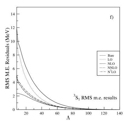
Figure 3: In a) the contributions to $H^{eff}-H$ from excitations in $Q$ above $\Lambda$ are plotted for a calculation with $\Lambda_{P}=8$ and $b$=1.7 fm. Each line describes the running of one of the 15 independent $P$-space matrix elements $\langle n^{\prime}l^{\prime}=0|H^{eff}-H|nl=0\rangle$, $1\leq n\leq n^{\prime}\leq 5$. Ten of the matrix elements are between nonedge states (solid), four connect the $n^{\prime}=5$ edge state to the $n$=1,2,3,4 nonedge states (dashed), and one is the diagonal $n^{\prime}=n=5$ edge-edge case (dot dashed). b)-e) show the residuals for naive LO, NLO, NNLO, and N³LO fits (see text). f) shows the RMS deviation for the set of $P$-space matrix elements. The expected systematic improvement with increasing order is apparent only for matrix elements between nonedge states.

III.1 The contact-gradient expansion for HOBET

The gradient with respect to the dimensionless coordinate $\vec{r}\equiv(\vec{r}_{1}-\vec{r}_{2})/b\sqrt{2}$ is denoted by $\overrightarrow{\nabla}$. The coefficients $a_{LO},a_{NLO},...$ in Table 1 then carry the dimensions of MeV.

The contact-gradient expansion defined in Table 1 is that commonly used in plane-wave bases, where one expands around $\vec{k}=0$ with

$$\left.\overrightarrow{\nabla}^{2}\exp{i\vec{k}\cdot\vec{r}}~{}\right|_{\vec{k}=0}=0.$$ (10)

HOBET begins with a lowest-energy $1s$ Gaussian wave packet with a characteristic momentum $\sim 1/b$. An analogous definition of gradients such that

$$\overrightarrow{\nabla}^{2}\psi_{1s}(b)=0$$ (11)

is obtained by redefining each operator appearing in Table 1 by

$$O\rightarrow\bar{O}\equiv e^{r^{2}/2}Oe^{r^{2}/2}.$$ (12)

The gradients appearing in the operators of Table 1 then act on polynomials in $r$. This leads to two attractive properties. First is the removal of operator mixing. Once $a_{LO}^{3S1}$ is fixed in LO to the $(n^{\prime},n)=(1,1)$ matrix element, this quantity remains fixed in NLO, NNLO, etc. Higher-order terms make no contributions to this matrix element. Similarly, $a_{NLO}$, once fixed to the $(1,2)$ matrix element, is unchanged in NNLO. That is, the NLO results contain the LO results, and so on. Second, this definition gives the HOBET effective interaction a simple dependence on nodal quantum numbers,

$$\overrightarrow{\nabla}^{2}\sim-4(n-1)~{}~{}~{}~{}~{}~{}~{}~{}\overrightarrow{\nabla}^{4}\sim 16(n-1)(n-2).$$ (13)

(The Appendix describes this expansion in some detail.) In each channel, this dependence agrees with the plane-wave result in lowest contributing order, but otherwise differs in terms of relative order $1/n$. This HO form of the contact-gradient expansion is connected with standard Talmi integrals talmi , generalized for nonlocal potentials, e.g.,

$$a_{LO} \sim \int^{\infty}_{0}\int^{\infty}_{0}e^{-r_{1}^{2}}\left[V(r_{1},r_{2})\right]e^{-r_{2}^{2}}r_{1}^{2}r_{2}^{2}dr_{1}dr_{2}$$

$$a_{NLO} \sim \int^{\infty}_{0}\int^{\infty}_{0}e^{-r_{1}^{2}}\left[r_{1}^{2}V(r_{1},r_{2})\right]e^{-r_{2}^{2}}r_{1}^{2}r_{2}^{2}dr_{1}dr_{2}=\int^{\infty}_{0}\int^{\infty}_{0}e^{-r_{1}^{2}}\left[V(r_{1},r_{2})r_{2}^{2}\right]e^{-r_{2}^{2}}r_{1}^{2}r_{2}^{2}dr_{1}dr_{2}$$ (14)

and so on.

III.2 Identifying terms with the contact-gradient expansion

The next question is the association of the operators in Table 1 with an appropriate set of terms in $H^{eff}-H$, so that the difficulties apparent in Fig. 3 are avoided. The reorganized BH equation of Eq. (2)

$$H^{eff} = {E\over E-TQ}\left[T-T{Q\over E}T+V+V{1\over E-QH}QV\right]{E\over E-QT}$$ (15)

$$\rightarrow {E\over E-TQ}\biggl{[}T-T{Q\over E}T+V+\sum_{i=LO,NLO,...}\bar{O}^{i}\biggr{]}{E\over E-QT}$$

isolates $V(E-QH)^{-1}QV$, a term that is sandwiched between short-range operators that scatter to high-energy states: one anticipates this term can be successfully represented by a short-range expansion like the contact-gradient expansion. This identification is made here and tested later in this paper.

This reorganization only affects the edge-state matrix elements, clearly. As the process of fitting coefficients uses matrix elements of low $(n^{\prime},n)$, none of which involves edge states, the coefficients are unchanged. But every matrix element involving edge states now includes the effects of rescattering by $QT$ to all orders. Thus a procedure for evaluating these matrix elements is needed.

III.3 Matrix element evaluation

There are several alternatives for evaluating Eq. (15) for edge states. One of these exploits the tri-diagonal form of $QT$ for the deuteron. If $|nl\rangle$ is an edge state in $P$ then

$${E\over E-QT}|n~{}l\rangle=|n~{}l\rangle+{1\over E-QT}QT|n~{}l\rangle=|n~{}l\rangle+\sqrt{n(n+l+1/2)}{1\over-\kappa^{2}-{2QT\over\hbar\omega}}|n+1~{}l\rangle$$ (16)

where $E<0$ for a bound state. The dimensionless parameter $\kappa=\sqrt{2|E|\over\hbar\omega}$ depends on the ratio of the binding energy $|E|$ to the HO energy scale. Note that the second vector on the right in Eq. (16) lies entirely in $Q$. Now

$${2\over\hbar\omega}QT|n+1~{}l\rangle = (2n+l+3/2)|n+1~{}l\rangle+\sqrt{(n+1)(n+l+3/2)}|n+2~{}l\rangle$$

$${2\over\hbar\omega}QT|n+2~{}l\rangle = \sqrt{(n+1)(n+l+3/2)}|n+1~{}l\rangle+(2n+l+7/2)|n+2~{}l\rangle+\sqrt{(n+2)(n+l+5/2)}|n+3~{}l\rangle$$

$${2\over\hbar\omega}QT|n+3~{}l\rangle = \sqrt{(n+2)(n+l+5/2)}|n+2~{}l\rangle+(2n+l+11/2)|n+3~{}l\rangle+\sqrt{(n+3)(n+l+7/2)}|n+4~{}l\rangle$$

$${2\over\hbar\omega}QT|n+4~{}l\rangle = ...$$ (17)

So the operator $2QT/\hbar\omega$ in the basis $\{|n+i~{}l\rangle,i=1,2,...$ } has the form

$${2\over\hbar\omega}QT=\left(\begin{array}[]{ccccc}\alpha_{1}&\beta_{1}&0&0&\\ \beta_{1}&\alpha_{2}&\beta_{2}&0&\\ 0&\beta_{2}&\alpha_{3}&\beta_{3}&\cdots\\ 0&0&\beta_{3}&\alpha_{4}&\\ &&\vdots&&\end{array}\right)$$ (18)

where

$$\alpha_{i}=\alpha_{i}(n,l)=2n+2i+l-1/2,~{}~{}~{}~{}\beta_{i}=\beta_{i}(n,l)=\sqrt{(n+i)((n+i+l+1/2)}~{}.$$ (19)

As is well known, if this representation of the operator $2QT/\hbar\omega$ is truncated after $k$ steps, the $2k-1$ nonzero coefficients {$\alpha_{i},\beta_{i}$} determine the $2k-1$ operator moments of the starting vector $|n+1~{}l\rangle$,

$$\langle n+1~{}l|\left({2QT\over\hbar\omega}\right)^{i}|n+1~{}l\rangle,~{}~{}~{}i=1,....,2k-1$$ (20)

A standard formula exists haydock for the moments expansion of the Green’s function acting on the first vector $|n+1~{}l\rangle$ of such a tri-diagonal matrix, allowing us to write

$$\sqrt{n(n+l+1/2)}{1\over-\kappa^{2}-{2QT\over\hbar\omega}}|n+1~{}l\rangle=\widetilde{g}_{1}(-\kappa^{2};n,l)|n+1~{}l\rangle+\widetilde{g}_{2}(-\kappa^{2};n,l)|n+2~{}l\rangle+\widetilde{g}_{3}(-\kappa^{2};n,l)|n+3~{}l\rangle+\cdots$$ (21)

The coefficients {$\widetilde{g}_{i}$} can be obtained from an auxiliary set of continued fractions {$g_{i}^{\prime}$} that are determined by downward recursion

$$g_{k}^{\prime}(-\kappa^{2};n,l) \equiv {1\over-\kappa^{2}-\alpha_{k}(n,l)}$$

$$g_{i-1}^{\prime}(-\kappa^{2};n,l) = {1\over-\kappa^{2}-\alpha_{i-1}(n,l)-\beta_{i-1}(n,l)^{2}g_{i}^{\prime}(-\kappa^{2};n,l)},~{}~{}i=k,....2$$ (22)

From these continued fractions the needed coefficients can be computed from the algebraic relations

$$\widetilde{g}_{1}(-\kappa^{2};n,l) = \sqrt{n(n+l+1/2)}g_{1}^{\prime}(-\kappa^{2};n,l)$$

$$\widetilde{g}_{i}(-\kappa^{2};n,l) = \widetilde{g}_{i-1}(-\kappa^{2};n,l)\beta_{i-1}g_{i}^{\prime}(-\kappa^{2};n,l),~{}~{}i=2,...,k$$ (23)

Defining $\widetilde{g}_{0}(-\kappa^{2};n,l)\equiv 1$ it follows

$${E\over E-QT}|n~{}l> = \sum_{i=0}^{k\rightarrow\infty}\widetilde{g}_{i}(-\kappa^{2};n,l)|n+i~{}l\rangle,~{}~{}\mathrm{edge~{}state}$$ (24)

$$= |n~{}l>,~{}~{}~{}~{}~{}~{}~{}~{}~{}~{}~{}~{}~{}~{}~{}~{}\mathrm{otherwise}$$

where it is understood that $k$ is made large enough so that the moments expansion for the Green’s function is accurate throughout the region in coordinate space where $E/(E-QT)|n~{}l\rangle$ is needed. Note that the first line of Eq. (24) can be viewed as the general result if one defines

$$g_{i}(-\kappa^{2};n,l)\equiv 0,~{}~{}i=1,...k,~{}~{}\mathrm{if}~{}|n~{}l\rangle~{}\mathrm{is~{}not~{}an~{}edge~{}state}.$$ (25)

(For $A\geq$ 3 one would be treating the 3($A$-1)-dimensional HO, with the role of the spherical harmonics replaced by the corresponding hyperspherical harmonics.) Eq. (24) can now be used to evaluate the various terms in Eq. (15).

Matrix elements for the contact-gradient operators: The matrix elements have the general form

$$\langle n^{\prime}l^{\prime}|{E\over E-TQ}\bar{O}{E\over E-QT}|nl\rangle=\sum_{i,j=0}\widetilde{g}_{j}(-\kappa^{2};n^{\prime},l^{\prime})\widetilde{g}_{i}(-\kappa^{2};n,l)\langle n^{\prime}+j~{}l|\bar{O}|n+i~{}l\rangle$$ (26)

where $\bar{O}$ is formed from gradients acting on the bra and ket, evaluated at $\vec{r}$=0. The general matrix element (any partial wave) is worked out in the Appendix. For example, one needs for $S$-wave channels the relation

$$(\vec{\nabla}^{2})^{p}e^{r^{2}/2}R_{nl=0}(r)Y_{00}(\Omega_{r})\big{|}_{\vec{r}\rightarrow 0}=(-4)^{p}~{}{(n-1)!\over(n-1-p)!}~{}{1\over\pi}\left[{\Gamma(n+1/2)\over(n-1)!}\right]^{1/2}$$ (27)

from which it follows

$$\langle n^{\prime}(l^{\prime}=0~{}S=1)J=1|{E\over E-TQ}\biggl{[}\sum_{i=LO,...,N^{3}LO}\bar{O}^{3S1,i}\biggr{]}{E\over E-QT}|n(l=0~{}S=1)J=1\rangle=$$

$${2\over\pi^{2}}\sum_{i,j=0}\widetilde{g}_{j}(-\kappa^{2};n^{\prime},l^{\prime}=0)\widetilde{g}_{i}(-\kappa^{2};n,l=0)\left[{\Gamma{n^{\prime}+j+1/2}\Gamma{n+i+1/2}\over(n^{\prime}+j-1)!(n+i-1)!}\right]\biggl{[}a_{LO}^{3S1}-4\left((n^{\prime}+j-1)+(n+i-1)\right)a_{NLO}^{3S1}$$

$$+16\left\{(n^{\prime}+j-1)(n+i-1)a_{NNLO}^{3S1,22}+\left((n^{\prime}+j-1)(n^{\prime}+j-2)+(n+i-1)(n+i-2)\right)a_{NNLO}^{3S1,40}\right\}$$

$$-64\left\{(n^{\prime}+j-1)(n+i-1)\bigl{(}(n^{\prime}+j-2)+(n+i-2)\bigr{)}a_{N^{3}LO}^{3S1,42}\right.$$

$$+\left.\left((n^{\prime}+j-1)(n^{\prime}+j-2)(n^{\prime}+j-3)+(n+i-1)(n+i-2)(n+i-3)\right)a_{N^{3}LO}^{3S1,60}\right\}\biggr{]}.$$ (28)

In the case of nonedge states, $\widetilde{g}_{i}\equiv 0$ except for the case of $\widetilde{g}_{0}\equiv 1$. Thus it is apparent that the net consequence of the rearrangement of the BH equation and the identification of the contact-gradient expansion with $V(E-QH)^{-1}QV$, is effectively a renormalization of the coefficients of that expansion for the edge HO states. That renormalization is governed by $\kappa^{2}=2|E|/\hbar\omega$, e.g.,

$$a_{LO}(n^{\prime},l^{\prime},n,l)\rightarrow a_{LO}^{\prime}(E;n^{\prime},l^{\prime},n,l)=a_{LO}(n^{\prime},l^{\prime},n,l)\sum_{i,j=0}\widetilde{g}_{j}(-\kappa^{2};n^{\prime},l^{\prime})\widetilde{g}_{i}(-\kappa^{2};n,l)$$

$$\times\left[{\Gamma(n^{\prime}+j+1/2)\Gamma(n+i+1/2)\over\Gamma(n^{\prime}+1/2)\Gamma(n+1/2)}\right]^{1/2}\left[{(n^{\prime}-1)!(n-1)!\over(n^{\prime}+j-1)!(n+i-1)!}\right]^{1/2}.$$ (29)

This renormalization is large, typically a reduction in strength by a factor of 2-4, for $|E|$=2.224 MeV, and also remains substantial for more deeply bound systems, as will be illustrated later. (The binding energy for this purpose is defined relative to the lowest particle breakup channel, the first extended state.) The effects encoded into $|\widetilde{\alpha}\rangle$ by summing $QT$ to all orders are nontrivial: they depend on a nonperturbative strong interaction parameter $|E|$ as well as $QT$, and they alter effective matrix elements of the strong potential. For a given choice of $\Lambda_{P}$, the renormalization depends on a single parameter, $2|E|/\hbar\omega$, not on $|E|$ or $b$ separately. In the plane-wave limit $b\rightarrow\infty$, this parameter is driven to $\infty$, so that $a_{LO}^{\prime}\rightarrow a_{LO}$. No renormalization is required in this limit. The dependence on $|E|$ is discussed in more detail later, including its connection to the state-dependence inherent in effective theory.

Matrix elements of the relative kinetic energy: The relative kinetic energy operator couples $P$ and $Q$ via strong matrix elements that grow as $n$. As Ref. luu discusses, this coupling causes difficulties with perturbative expansions in $H$ even in the case of $P$ spaces that contain almost all of the wave function (e.g., $\Lambda_{P}\sim$ 70). There is always a portion of the wave function tail at large $r$ that is nonperturbative, involving matrix elements of $T$ that exceed $\Lambda_{P}\hbar\omega/2$.

The kinetic energy contribution is

$$\langle\alpha|T+T{1\over E-QT}QT|\beta\rangle=\langle\widetilde{\alpha}|T-T{Q\over E}T|\widetilde{\beta}\rangle=\langle\alpha|T|\widetilde{\beta}\rangle=\langle\widetilde{\alpha}|T|\beta\rangle$$ (30)

where the last two terms show that the transformation to states $|\widetilde{\alpha}\rangle=E/(E-QT)|\alpha\rangle$ reduces the calculation of the rescattering to that of a bare matrix element. It follows from this expression

$$\langle n^{\prime}~{}l|T+T{1\over E-QT}QT|n~{}l\rangle=\langle n^{\prime}~{}l|T|n~{}l\rangle+{\hbar\omega\over 2}\delta_{n^{\prime}n}\sqrt{n(n+l+1/2)}\widetilde{g}_{1}(-\kappa^{2};n,l).$$ (31)

Thus, rescattering via $QT$ alters the diagonal matrix element of the effective interaction for edge states, as determined by $\widetilde{g}_{1}(-\kappa^{2};n,l)$.

Matrix elements of the bare potential: The $P$-space matrix element of $V$ becomes $\langle\widetilde{\alpha}|V|\widetilde{\beta}\rangle$ which, as is illustrated in Fig. 2, involves an integral over a wave function that, apart from normalization, differs from the HO only in the tail, where the potential is weak. It can be evaluated by generating the wave functions $|\widetilde{\alpha}\rangle$ and $|\widetilde{\beta}\rangle$ as HO expansions,

$$\left[\sum_{j=0}\widetilde{g}_{j}(-\kappa^{2};n^{\prime},l^{\prime})\langle n^{\prime}+j~{}l^{\prime}|\right]~{}V~{}\left[\sum_{i=0}|n+i~{}l\rangle\widetilde{g}_{i}(-\kappa^{2};n,l)\right]=\sum_{i,j=0}\widetilde{g}_{j}(-\kappa^{2};n^{\prime},l^{\prime})\widetilde{g}_{i}(-\kappa^{2};n,l)\langle n^{\prime}+j~{}l^{\prime}|~{}V~{}|n+i~{}l\rangle.$$ (32)

though the alternative Green’s function expression, discussed below, is simpler.

Use of the free Green’s function: An alternative to an expansion in an HO basis is generation of $|\widetilde{\alpha}\rangle$ with the free (modified Helmholtz) Green’s function. For any P-space state $|n~{}l\rangle$,

$$(E-QT)|\widetilde{\alpha}\rangle=E|\alpha\rangle~{}\Rightarrow~{}(E-T)|\widetilde{\alpha}\rangle=E|\alpha\rangle-PT|\widetilde{\alpha}\rangle$$ (33)

That is, both $E-QT$ and $E-T$ project $|\widetilde{\alpha}\rangle$ back into the $P$-space. The free Green’s function equation can be written

$$(E-T)|\widetilde{\alpha}\rangle = P\left[E-T{E\over E-QT}\right]P|\alpha\rangle$$ (34)

$$= \left[P{1\over E-T}P\right]^{-1}|\alpha\rangle.$$

Either of the driving terms on the right-hand side is easy to manipulate. The second expression requires inversion of a P-space matrix, one most easily calculated in momentum space, as the HO is its own Fourier transform and as the resulting momentum-space integrals can be done in closed form. This form was used in the three-body calculations of Ref. tom .

Here I will use the first expression above, rewriting the right-hand-side driving term in terms of $|\alpha_{nlm_{l}}\rangle$,

$$P\left[E-T{E\over E-QT}\right]P|\alpha\rangle={\hbar\omega\over 2}\biggl{[}\biggl{(}-\kappa^{2}-(2n+l-1/2)-\widetilde{g}_{1}(-\kappa^{2};n,l)\sqrt{n(n+l+1/2)}\biggr{)}|n~{}l~{}m_{l}>$$

$$-\sqrt{(n-1)(n+l-1/2)}|n-1~{}l~{}m_{l}\rangle-\sqrt{n(n+l+1/2)}P|n+1~{}l~{}m_{l}\rangle\biggr{]}\equiv{\hbar\omega\over 2}|\alpha_{nlm_{l}}\rangle,$$ (35)

where the driving term has been kept general, valid for either edge or nonedge states: the latter can be a helpful numerical check, verifying that a HO wave function is obtained, for such cases, from the expression below. For an edge state, $\widetilde{g}_{1}$ is nonzero and $P|n+1~{}l\rangle\equiv 0$; for a nonedge state, $\widetilde{g}_{1}=0$ and $P$=1. Labeling the corresponding edge state as $|\widetilde{\alpha}_{nlm_{l}}\rangle$,

$$\langle\vec{r}|\widetilde{\alpha}_{nlm_{l}}\rangle = \int d^{3}\vec{r}^{~{}\prime}{1\over 4\pi|\vec{r}-\vec{r}^{~{}\prime}|}e^{-\kappa|\vec{r}-\vec{r}^{~{}\prime}|}~{}\langle\vec{r}^{~{}\prime}|\alpha_{nlm_{l}}>$$ (36)

$$= -Y_{lm}(\Omega_{r})\biggl{[}{1\over\sqrt{r}}~{}I_{l+1/2}(\kappa r)\int_{r}^{\infty}d^{3}\vec{r}^{~{}\prime}(r^{\prime})^{3/2}K_{l+1/2}(\kappa r^{\prime})~{}\langle\vec{r}^{~{}\prime}|\alpha_{nlm_{l}}>$$

$$+{1\over\sqrt{r}}~{}K_{l+1/2}(\kappa r)\int_{0}^{r}d^{3}\vec{r}^{~{}\prime}(r^{\prime})^{3/2}I_{l+1/2}(\kappa r^{\prime})~{}\langle\vec{r}^{~{}\prime}|\alpha_{nlm_{l}}>$$

where $I$ and $K$ denote the standard modified Bessel functions. By expressing the HO radial wave functions in terms of the underlying Laguerre polynomials and integrating the polynomials term by term, alternative expressions are obtained for the various quantities previously expressed as expansions in the $\widetilde{g}_{i}$. This is detailed in the Appendix. One finds, for example,

$$\langle\vec{r}=0|\widetilde{\alpha}_{nlm_{l}}\rangle = \delta_{l,0}~{}\delta_{m_{l},0}~{}\sqrt{{(n-1)!\Gamma(n+1/2)\over 2\pi}}~{}\sum_{k=0}^{n}{(-2)^{k}\over k!(n-k)!\Gamma(k+3/2)}~{}\times$$ (37)

$$\biggl{[}(n-k)(\kappa^{2}+3n-3/2-k+\widetilde{g}_{1}(-\kappa^{2};n,0)\sqrt{n(n+1/2)})+P[n+1,l=0]n(n+1/2)\biggr{]}~{}\times$$

$$\biggl{[}-\sqrt{2}~{}\kappa~{}\Gamma(k+3/2)~{}{}_{1}F_{1}[k+3/2;3/2;\kappa^{2}/2]+k!~{}{}_{1}F_{1}[k+1;1/2;\kappa^{2}/2]\biggr{]}$$

where ${}_{1}F_{1}$ is Kummer’s confluent hypergeometric function, and where $P[n+1,l=0]=1$ if $|n+1~{}l\rangle$ is in $P$, and 0 otherwise. Similar expressions can be derived to handle all of the operators $\bar{O}$ appearing in the contact-gradient expansion (see the Appendix).

III.4 Numerical Tests

In this subsection channel-by-channel N³LO results are presented for $H^{eff}$ based on Eqs. (12) and (15), which isolate a short-range operator that plausibly can be accurately and systematically expanded via contact-gradient operators.

For $\Lambda_{P}=8$, the fitting procedure determines all N³LO coefficients from nonedge matrix elements, leaving all edge matrix elements and a substantial set of nonedge matrix elements unconstrained. Thus one can use these matrix elements to test whether the expansion systematically accounts for the “data,” the set of numerically generated $v_{18}$ matrix elements of $H^{eff}$. One test is the running of the results as a function of $\Lambda$: a systematic progression through LO, NLO, etc., operators should be observed as $\Lambda$ is lowered to the SM scale. A second test is the “Lepage plot” lepage , which displays residual errors in matrix elements: if the improvement is systematic, these residual errors should reflect the nodal-quantum-number dependence of the operators that would correct these results, in next order.

Eq. (15) includes “bare” terms – the matrix elements $\langle\alpha|T|\widetilde{\beta}\rangle$ and $\langle\widetilde{\alpha}|V|\widetilde{\beta}\rangle$ – and a term involving repeated scattering by $H$ in $Q$, but sandwiched between the short-range operator $QV$. To test the dependence on $\Lambda$, the rescattering term is decomposed in the manner of Eq. (9),

$$\Delta_{QT}(\Lambda)={E\over E-TQ}\left[V{1\over E-QH}QV-V{1\over E-Q_{\Lambda}H}Q_{\Lambda}V\right]{E\over E-QT},$$

to isolate the contribution of scattering above the scale $\Lambda.$ $\Delta_{QT}(\Lambda)$ is evaluated numerically for $v_{18}$ at each required $\Lambda.$ The long-wavelength summation is always done to all orders – the running with $\Lambda$ thus reflects the behavior of the short-range piece, $V(E-QH)^{-1}QV$. The full $P$-space effective interaction is obtained as $\Lambda\rightarrow\Lambda_{P}$.

Figure 4: As in Fig. 3, but for the $QT$-summed reordering of $H^{eff}$. The contributions to the effective interaction from excitations in $Q$ above $\Lambda$, denoted $\Delta_{QT}(\Lambda)$ in the text, are plotted. Each line gives the running of a $P$-space matrix element. b)-e) show the residuals for LO, NLO, NNLO, and N³LO fits (see text). f) shows the RMS deviation for the set of $P$-space matrix elements. The improvement with increasing order is systematic and rapid: at N³LO the RMS deviation for unconstrained matrix elements as $\Lambda\rightarrow\Lambda_{P}$ is about 3 keV. That is, the entire effective interaction is reproduced to a few parts in 10⁴.

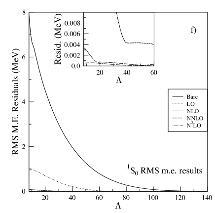
Figure 5: As in Fig. 4, but for the ${}^{1}S_{0}$ channel. The N³LO results are seen to reproduce the entire effective interaction to the accuracy of about a keV, or one part in $10^{4}$.

As outlined before, coefficients are fitting to the longest wavelength information. For example, in $S$ channels, $a_{LO}$ is fixed to the $(n^{\prime},n)$ = (1,1) matrix element; the absence of operator mixing then guarantees this coefficient remains fixed, as higher order terms are evaluated. The single $a_{NLO}$ coefficient is fixed to (2,1) (or equivalently (1,2)) ; $a_{NNLO}^{22}$ and $a_{NNLO}^{40}$ are determined from (2,2) and (3,1); and finally $a_{N^{3}LO}^{42}$ and $a_{N^{3}LO}^{60}$ are fixed to (3,2) and (4,1). So at N³LO there are a total of 6 parameters. This procedure is repeated for a series of $\Lambda$ ranging from 140 to $\Lambda_{P}$=8. The results in each order, and the improvement order by order, are thus obtained as a function of $\Lambda$. $P$ contains 15 independent matrix elements in the ${}^{3}S_{1}-{}^{3}S_{1}$ channel, nine of which play no role in the fitting: these test whether the improvement is systematic.

Figures 4 and 5 show the results for ${}^{3}S_{1}-{}^{3}S_{1}$ and ${}^{1}S_{0}-{}^{1}S_{0}$. Panel a) shows the evolution of the matrix elements $\langle\alpha|\Delta_{QT}(\Lambda)|\beta\rangle$ for each of the 15 independent matrix elements. Matrix elements involving only nonedge states, a single edge state, or two edge states are denoted by solid, dashed, and dash-dotted lines, respectively. Progressively more binding is recovered as $\Lambda\rightarrow\Lambda_{P}$. In the ${}^{3}S_{1}-{}^{3}S_{1}$ case, the contribution at $\Lambda_{P}$ is $\sim$ 12-14 MeV for nonedge matrix elements, $\sim$ 7-8 MeV for matrix elements with one edge state, and $\sim$ 5 MeV for the $\langle n=5l=0|\Delta_{QT}(\Lambda_{P})|n=5l=0\rangle$ double-edge matrix element.

Panels b)-e) show the residuals – the difference between the matrix elements of $\Delta_{QT}(\Lambda_{P})$ and those of the contact-gradient potential of Eq. (15) – from LO through N³LO. The trajectories correspond to the unconstrained matrix elements (14 in LO, 9 in N³LO): the fitted matrix elements produce the horizontal line at 0. Unlike the naive approach in Fig. 3, the improvement is now systematic in all matrix elements. In the ${}^{3}S_{1}-{}^{3}S_{1}$ channel, a LO treatment effectively removes all contributions in $Q$ above $\Lambda\sim$ 60; NLO lowers this scale to $\sim$ 40, and NNLO is $\sim$ 20. The magnitude of N³LO residuals at $\Lambda_{P}$ is typically $\mathrel{\hbox to0.0pt{\lower 4.0pt\hbox{\hskip 1.0pt$\sim$}\hss}\raise 1.0pt\hbox{$<$}}$ 2 keV – the entire effective interaction can be represented by Eq. (15) to an accuracy of about 0.01%. Panel f) shows the root mean square (RMS) deviation among the unconstrained matrix elements, and the rapid order-by-order improvement.

The pattern repeats in the ${}^{1}S_{0}-{}^{1}S_{0}$ channel, where the convergence (in terms of the size of the residuals) is somewhat faster. The N³LO RMS deviation among the unconstrained matrix elements at $\Lambda_{P}$ is $\sim$ 0.5 keV.

Figure 6: As in Figs. 4 and 5, but for the ${}^{3}S_{1}-{}^{3}D_{1}$ channel. As with the cases described before, the N³LO results remain accurate at the few keV level, as the integration is brought down to the shell-model scale, $\Lambda\rightarrow\Lambda_{P}$.

Figure 7: As in Fig. 4, but for the ${}^{3}D_{1}$ channel.

Figure 8: As in Fig. 4, but for the ${}^{3}D_{2}$ channel.

Figure 9: As in Fig. 7 and 8, but for the ${}^{3}D_{3}$ channel. This “stretched” configuration generates much larger residuals than the other $l=2$ channels. Consequently a calculation to N⁴LO would be needed to reduce typical matrix element errors to $\sim$ 10 keV, in the limit $\Lambda\rightarrow\Lambda_{P}$.

Figure 10: As in Fig. 4, but for the ${}^{1}D_{2}$ channel.

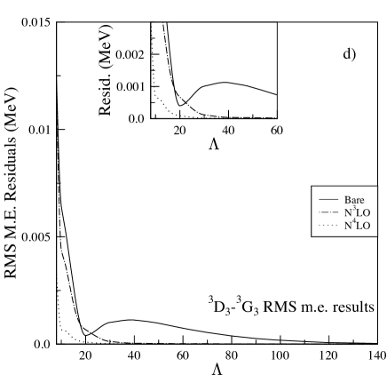
Figure 11: As in Fig. 4, but for the ${}^{3}D_{3}-{}^{3}G_{3}$ channel. The N⁴LO contribution is also shown.

The remaining positive-parity channels that can be constrained at N³LO are given in Figs. 6 through 11: ${}^{3}S_{1}-{}^{3}D_{1}$ (leading order contribution NLO); ${}^{1}D_{2}-{}^{1}D_{2}$, ${}^{3}D_{1}-{}^{3}D_{1}$, ${}^{3}D_{2}-{}^{3}D_{2}$, and ${}^{3}D_{3}-{}^{3}D_{3}$ (NNLO); and ${}^{3}D_{3}-{}^{3}G_{3}$ (N³LO).

Table 2 gives the resulting fitted couplings at N³LO for all contributing channels, along with numerical results for the root-mean-square $Q$-space contributions to $\Delta_{QT}(\Lambda_{P})$ and the root-mean-square residuals (the deviation between the contact-gradient prediction and $\Delta_{QT}(\Lambda_{P})$ for the remaining unconstrained effective interactions matrix elements). The quality of the agreement found in the ${}^{1}S_{0}$ and ${}^{3}S_{1}$channels is generally typical – residuals at the few kilovolt level – though there are some exceptions and some general patterns that emerge. One of these is the tendency of the triplet channels with spin and angular momentum aligned (${}^{3}S_{1}-{}^{3}S_{1}$, ${}^{3}P_{2}-{}^{3}P_{2}$, ${}^{3}D_{3}-{}^{3}D_{3}$, and ${}^{3}F_{4}-{}^{3}F4$) to exhibit larger residuals than the remaining $S,P,D$ and $F$ channels, respectively. The ${}^{3}D_{3}-{}^{3}D_{3}$, which has contributions at NNLO and N³LO, stands out as the most difficult channel, with a residual of 122 keV, one to two orders of magnitude greater than the typical scale of N³LO residuals.

Table 2: The effective interaction for LO through N³LO, with $\Lambda_{P}=8$ and $b$=1.7 fm.^†

Channel	Couplings (MeV)							$\langle$M.E.$\rangle_{RMS}$ (MeV)	$\langle$Resid.$\rangle_{RMS}$ (keV)
	$a_{LO}^{S}$	$a_{NLO}^{S}$	$a_{NNLO}^{S,22}$	$a_{NNLO}^{S,40}$	$a_{N^{3}LO}^{S,42}$	$a_{N^{3}LO}^{S,60}$
${}^{1}S_{0}-{}^{1}S_{0}$	-32.851	-2.081E-1	-2.111E-3	-1.276E-3	-7.045E-6	-1.8891E-6		7.94	0.53
${}^{3}S_{1}-{}^{3}S_{1}$	-62.517	-1.399	-5.509E-2	-1.160E-2	-5.789E-4	-1.444E-4		11.97	2.71
		$a_{NLO}^{SD}$	$a_{NNLO}^{SD,22}$	$a_{NNLO}^{SD,04}$	$a_{N^{3}LO}^{SD,42}$	$a_{N^{3}LO}^{SD,24}$	$a_{N^{3}LO}^{SD,06}$
${}^{3}S_{1}-{}^{3}D_{1}$		2.200E-1	1.632E-2	2.656E-2	2.136E-4	3.041E-4	-1.504E-4	0.160	2.45
			$a_{NNLO}^{D}$		$a_{N^{3}LO}^{D}$
${}^{1}D_{2}-{}^{1}D_{2}$			-6.062E-3		-1.189E-4			0.027	1.21
${}^{3}D_{1}-{}^{3}D_{1}$			-1.034E-2		-1.532E-4			0.051	2.27
${}^{3}D_{2}-{}^{3}D_{2}$			-3.048E-2		-5.238E-4			0.141	1.20
${}^{3}D_{3}-{}^{3}D_{3}$			-9.632E-2		-4.355E-3			0.303	122‡
					$a_{N^{3}LO}^{SD}$
${}^{3}D_{3}-{}^{3}G_{3}$					3.529E-4			0.012	12.2‡
		$a_{NLO}^{P}$	$a_{NNLO}^{P}$		$a_{N^{3}LO}^{P,33}$	$a_{N^{3}LO}^{P,51}$
${}^{1}P_{1}-{}^{1}P_{1}$		-8.594E-1	-7.112E-3		-6.822E-5	1.004E-5		0.694	0.11
${}^{3}P_{0}-{}^{3}P_{0}$		-1.641	-1.833E-2		-2.920E-4	-1.952E-4		1.283	2.26
${}^{3}P_{1}-{}^{3}P_{1}$		-1.892	-1.588E-2		-1.561E-4	-6.737E-6		1.526	0.08
${}^{3}P_{2}-{}^{3}P_{2}$		-4.513E-1	-1.257E-2		-5.803E-4	-1.421E-4		0.285	5.61
			$a_{NNLO}^{PF}$		$a_{N^{3}LO}^{PF,33}$	$a_{N^{3}LO}^{PF,15}$
${}^{3}P_{2}-{}^{3}F_{2}$			-4.983E-3		1.729E-5	-5.166E-5		0.034	1.43
					$a_{N^{3}LO}^{F}$
${}^{1}F_{3}-{}^{1}F_{3}$					-3.135E-4			0.007	1.03
${}^{3}F_{2}-{}^{3}F_{2}$					-8.537E-4			0.020	2.34
${}^{3}F_{3}-{}^{3}F_{3}$					-2.647E-4			0.006	0.61
${}^{3}F_{4}-{}^{3}F_{4}$					-5.169E-4			0.008	6.23

Figures 12 through 18 show the convergence for the various channels involving odd-parity states and contributing through N³LO: ${}^{1}P_{1}-{}^{1}P_{1}$, ${}^{3}P_{J}-{}^{3}P_{J}$, ${}^{3}P_{2}-{}^{3}F_{2}$, ${}^{1}F_{3}-{}^{1}F_{3}$, and ${}^{3}F_{J}-{}^{3}F_{J}$. While the spin-aligned channels show slightly large residuals, overall the RMS errors at N³LO are at the one-to-few keV level. Thus a simple and essentially exact representation for the effective interaction exists.

Figure 12: As in Fig. 4, but for the ${}^{1}P_{1}$ channel.

Figure 13: As in Fig. 4, but for the ${}^{3}P_{0}$ channel.

Figure 14: As in Fig. 4, but for the ${}^{3}P_{1}$ channel.

Figure 15: As in Fig. 4, but for the ${}^{3}P_{2}$ channel.

Figure 16: As in Fig. 4, but for the ${}^{3}P_{2}-{}^{3}F_{2}$ channel.

Figure 17: The lowest contributing order to the $1F_{3}$ channel is N³LO. $\Delta_{QT}(\Lambda)$ and the N³LO residuals for the five unconstrained matrix elements are shown.

Figure 18: As in Fig. 17, but for the ${}^{3}F_{J}-{}^{3}F_{J}$ channels. As has been noted in other cases, the stretched ${}^{3}F_{4}$ case has the largest residual.

Expansion parameters, naturalness: The approach followed here differs from EFT, where the formalism is based on an explicit expansion parameter, the ratio of the momentum to a momentum cutoff. The input into the present calculation is a set of numerical matrix elements of an iterated, nonrelativistic potential operating in $Q$. Potentials like $v_{18}$ are also effectively regulated at small $r$ by some assumed form, e.g., a Gaussian, matched smoothly to the region in $r$ that is constrained by scattering data. Thus there are no singular potentials iterating in $Q$.

Intuitively it is clear that the convergence apparent in Table 2 is connected with the range of hard-core interactions (once edge states are transformed by summing $T$). A handwaving argument can be made by assuming rescattering in $Q$ effectively generates a potential of the form

$$V_{0}e^{-r_{12}^{2}/a^{2}},$$

where $r_{12}=|\vec{r_{1}}-\vec{r_{2}}|$. This ansatz is local, so there is some arbitrariness in mapping it onto contact-gradient expansion coefficients, which correspond to the most general nonlocal potential. But a sensible prescription is to equate terms with equivalent powers of $r^{2}$, in the bra and ket, when taking HO matrix of this potential. Then one finds, for S-wave channels

$$a(m^{\prime},m)\equiv a_{N^{m^{\prime}+m}LO}^{S,2m^{\prime}2m}={1\over 4^{m^{\prime}+m}m^{\prime}!m!}{(2m^{\prime}+2m+1)!!\over(2m^{\prime}+1)!!(2m+1)!!}V_{0}\left[{\pi a^{2}\over a^{2}+2b^{2}}\right]^{3/2}\left[a^{2}\over a^{2}+2b^{2}\right]^{m^{\prime}+m}$$ (38)

where $b$ is the oscillator parameter. (The notation is such that, e.g., $a(m^{\prime}=3,m=0)=a_{N^{3}LO}^{S,60}$.) The last term is thus the expansion parameter: if the range of the hard-core physics residing in $Q$ is small compared to the natural nuclear size scale $b$, then each additional order in the expansion should be suppressed by $\sim(a/b)^{2}$.

One can use this crude ansatz to assess whether the convergence shown in Table 2 is natural, or within expectations. The LO and NLO ${}^{1}S_{0}-{}^{1}S_{0}$ results effectively determine $V_{0}$ and $a$; thus the strengths of four NNLO and N³LO potentials can be predicted relative to that of $a_{LO}$ and $a_{NLO}$. The predicted hierarchy $a_{LO}:a_{NLO}:a_{NNLO}^{22}:a_{NNLO}^{40}:a_{N^{3}LO}^{42}:a_{N^{3}LO}^{60}$ of

$$1:6.3\times 10^{-3}:6.7\times 10^{-5}:2.0\times 10^{-5}:3.0\times 10^{-7}:4.2\times 10^{-8}$$

matches the relative strengths of the couplings in the table quite well,

$$1:6.3\times 10^{-3}:6.4\times 10^{-5}:3.9\times 10^{-5}:2.1\times 10^{-7}:5.7\times 10^{-8},$$

including qualitatively reproducing the ratios of the two NNLO and two N³LO coefficients. The parameters derived from $a_{LO}$ and $a_{NLO}$ are $a\sim 0.39$ fm and $V_{0}\sim-1.5$ GeV. In the ${}^{1}S_{0}$ channel the bare Argonne $v_{18}$ potential at small $r$ can be approximated by a Gaussian with $a\sim 0.33$ fm and $V_{0}\sim 3.0$ GeV. So again the crude estimates of range and even the strength are not unreasonable. [Note that the signs of the two $V_{0}$s are correct – the $P$-space lacks the appropriate short-range repulsion and thus samples the iterated bare potential at small $r$, a contribution that then must be subtracted off when $H^{eff}$ is evaluated.]

A similar exercise in the ${}^{3}S_{1}$ channel yields the predicted hierarchy

$$1:2.2\times 10^{-2}:8.3\times 10^{-4}:2.5\times 10^{-4}:13.1\times 10^{-6}:1.9\times 10^{-6}$$

which compares with the coupling ratios calculated from Table 2

$$1:2.2\times 10^{-2}:8.8\times 10^{-4}:1.9\times 10^{-4}:9.3\times 10^{-6}:2.3\times 10^{-6}.$$

The convergence is very regular but slower: in this case the effective Gaussian parameter needed to describe these trend is $a\sim 0.75$ fm. The overall strength, $V_{0}\sim-0.42$, differs substantially from that found for the ${}^{1}S_{0}$ channel, though the underlying $v_{18}$ potentials for ${}^{3}S_{1}-{}^{3}S_{1}$ and ${}^{1}S_{0}-{}^{1}S_{0}$ scattering are quite similar (see Fig. 19).

The ${}^{3}S_{1}-{}^{3}S_{1}$ behavior is similar to that found in the other spin-aligned channels, such as ${}^{3}D_{3}-{}^{3}D_{3}$ and ${}^{3}P_{2}-{}^{3}P_{2}$, where the scattering in $Q$ includes contributions from the tensor force. The tensor force contributes to the LO s-wave coupling through intermediate $D$-states in $Q$, e.g.,

$$\langle n^{\prime}l^{\prime}=0|V_{SD}Q|n^{\prime\prime}l=2\rangle{1\over\langle E\rangle}\langle n^{\prime\prime}l=2|QV_{SD}|nl=0\rangle,$$

as the product of two tensor operators has an s-wave piece. The radial dependence of $V_{SD}$ for $v_{18}$, shown in Fig. 19, is significantly more extended than in central-force ${}^{3}S_{1}-{}^{3}S_{1}$ and ${}^{1}S_{0}-{}^{1}S_{0}$ cases. This has the consequences that (1) the mean excitation energy $\langle E\rangle$ for ${}^{3}S_{1}-{}^{3}D_{1}$ will be lower (enhancing the importance of the tensor force) and (2) the $P$-space $\langle^{3}S_{1}|H^{eff}|^{3}S_{1}\rangle$ matrix element will reflect the extended range.

Once this point is appreciated – that the effective expansion parameter are naturally channel-dependent because of effects like the tensor force – the results shown in Table 2 are very pleasing:

• In each channel the deduced couplings $a_{LO},~{}a_{NLO},~{}a_{NNLO},~{}a_{N^{3}LO},...$ evolve in a very orderly, or natural, fashion: one can reliably predict the size of the next omitted term. The convergence appears related to an effective range characterizing scattering in $Q$.

• The convergence varies from channel to channel, but this variation reflects underlying physics, such as role of the tensor force, governing the channel’s range. One does not find, nor perhaps should one expect to find, some single parameter $p/\Lambda$ to characterize convergence independent of channel.

• The convergence is very satisfactory in all channels: the measure used in Table 2, $\langle$Resid.$\rangle_{RMS}$, is an exceedingly conservative one, as discussed below. But even by by this standard, in only one channel (${}^{3}D_{3}-{}^{3}D_{3}$) do the RMS residual discrepancies among unconstrained matrix elements exceed $\sim$ 10 keV. Given the arguments above, it is perfectly sensible to work to order NNLO in rapidly-converging channels like ${}^{1}S_{0}-{}^{1}S_{0}$ and N⁴LO in slowly converging channels like ${}^{3}D_{3}-{}^{3}D_{3}$. As noted in the table, at N⁴LO the residual in the ${}^{3}D_{3}-{}^{3}D_{3}$ channel is reduced to 22 keV.

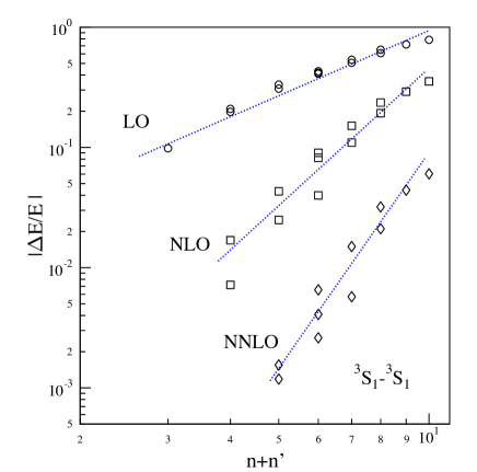
Figure 19: (Color online) The left panel shows the radial dependence of the Argonne $v_{18}$ potential in the ${}^{1}S_{0}-{}^{1}S_{0}$, ${}^{3}S_{1}-{}^{3}S_{1}$, and ${}^{3}S_{1}-{}^{3}D_{1}$ (tensor) channels. The last is clearly more extended. The right panel is a “Lepage plot” displaying fractional errors as a function of the order of the calculation, on log scales. The steepening of the slope with order is the sign of a well behaved, converging effective theory.

Convergence and the “Lepage” plot: The procedure often followed in an effective theory is to use information about the low-lying excitations to parameterize an effective Hamiltonian, which is then used to predict properties of other states near the ground state. In contrast, the goal here has been to characterize the entire effective interaction to high accuracy. As described below, the residual errors in the procedure are typically dominated by matrix elements with the largest $n$ and $n^{\prime}$, corresponding to minor components in the deuteron ground state, for example. The difference in the deuteron binding energy using exact matrix elements of $H^{eff}$ versus using the N³LO expansion is quite small ($\sim$ 40 eV).

Order-by-order improvement should be governed by nodal quantum numbers. For example, in LO in the ${}^{3}S_{1}$ channel the omitted NLO term would be

$$-{8a_{NLO}^{3S1}\over\pi^{2}}(n^{\prime}+n-2)\left[{\Gamma[n^{\prime}+1/2]\Gamma[n+1/2]\over(n^{\prime}-1)!(n-1)!}\right]^{1/2}\stackrel{{\scriptstyle n^{\prime},n~{}\mathrm{large}}}{{\longrightarrow}}-{2a_{NLO}^{3S1}\over\pi^{2}}\left[(4n^{\prime}-1)(4n-1)\right]^{1/2}(n^{\prime}+n-2)$$ (39)

Thus the fractional error associated with the omission of the NLO terms relative to LO should to be linear in the sum of the nodal quantum numbers, if the expansion is capturing the correct physics. That is, the expected absolute (e.g., in keV) error for ($n^{\prime},n$)=(5,5) would be about 16 times that for (1,2).

In higher orders this distinction between large and small $n$ grows. At LO+NLO, the expected fractional errors in matrix elements from omitted NNLO terms would be quadratic in $n$ and $n^{\prime}$: the explicit functional dependence is no longer simple as there are two NNLO operators, and one would not know a priori the relevant quadratic combination of $n^{\prime}$ and $n$ governing the error. At NNLO the fractional error would be a cubic polynomial in $n$ and $n^{\prime}$.

While beyond LO the expected fractional errors have a dependence on both $n$ and $n^{\prime}$, it is still helpful to display results as a 2D “Lepage plot” using $n+n^{\prime}$ – proportional to the average $\langle p^{2}\rangle$ of bra and ket – as the variable. Such a plot makes clear whether improved fits in an effective theory are systematic – that is, due to a correct description of the underlying physics, not just additional parameters. The use of a single parameter, $n+n^{\prime}$, of course maps multiple matrix elements onto the same $x$ coordinate, when the ET indicates this is a bit too simple beyond LO. Nevertheless, the right panel in Fig. 19 still shows rather nicely that the nuclear effective interactions problem is a very well behaved effective theory. In LO the residual errors do map onto the single parameter $n+n^{\prime}$ to very good accuracy, and the residual error is linear. The steepening of the convergence with order is consistent with the expected progression from linear to quadratic to cubic behavior in nodal quantum numbers. By NNLO, errors in unconstrained matrix elements for small $n+n^{\prime}$ are tiny, compared to those with high $n+n^{\prime}$. That is, the expansion converges most rapidly for matrix elements between long-wavelength states, as it should. However, improvement is substantial and systematic everywhere, including at the largest $n+n^{\prime}$.

IV Properties and Energy Dependence of the Effective Interaction

The results of the previous section demonstrate the existence of a simple systematic operator expansion for the HOBET effective interaction. Its behavior order-by-order and in the Lepage plot indicates that the short-wavelength physics is being efficiently captured in the associated operator coefficients.

The error measure used in the N³LO fit is dominated by the absolute errors in matrix elements involving the highest nodal quantum numbers: these matrix elements are large even though they may not play a major role in determining low-lying eigenvalues. (It might have been better to use the fractional error in matrix elements, a measure that would be roughly independent of $n^{\prime}$ and $n$.) Other possible measures of error are the ground state energy; the first energy-moment of the effective interaction matrix (analogous to the mean eigenvalue in the SM); the fluctuation between neighboring eigenvalues of that matrix (analogous to the level spacing in the SM); and the overlap of the eigenfunctions of that matrix with the exact eigenfunctions (analogous to wave function overlaps in the SM). The N³LO interaction in the coupled ${}^{3}S_{1}-{}^{3}D_{1}$ channel produces a ground state energy accurate to $\sim$ 40 eV; a spectral first moment accurate to 1.81 keV; an RMS average deviation in the level spacing of 3.52 keV; and wave function overlaps that are unity to better than four significant digits. As rescattering in $Q$ contributes $\sim$ -10 MeV to eigenvalues, the accuracy of the N³LO representation of the effective interaction is, by these spectral measures, on the order of 0.01%. As the best excited-state techniques in nuclear physics currently yield error bars of about 100 keV for the lightest nontrivial nuclei, this representation of the two-body effective interaction is effectively exact argonne ; nocore .

The approach requires one to sum $QT$ to all orders, producing a result that depends explicitly on $|E|$ – which in this context should be measured relative to the first breakup channel. While the associated effects increase with decreasing $|E|$, it will be shown later that the renormalization is substantial even for well-bound nuclear states. The deuteron is definitely not an extreme case. The effects are also sensitive to the choice of $P$, through $b$, which controls the mean momentum within $P$ – a small $b$ reduces the missing hard-core physics, but exacerbates the problems at long wavelengths, and conversely. Figure 1 suggests factor-of-two changes in the $Q$-space contribution to the deuteron binding energy can result from $\sim$ 20% changes in $b$. At the outset, the dependence on $|E|$ and $b$ seems like a difficulty for nuclear physics, as modest changes in these parameters alter predictions.

One of the marvelous properties of the HO is that the $QT$ sum can be done. The two effects discussed above turn out to be governed by a single parameter, $\kappa$. The associated effects are nonperturbative in both $QT$ and $QV$. In the case of $QT$ an explicit sum to all orders is done. The effects are also implicitly nonperturbative in $QV$, because of the dependence on $|E|$. This is why the BH approach is so powerful: because $|E|$ is determined self-consistently, it is simple to incorporate this physics directly into the iterative process (which has been shown to converge very rapidly in the HOBET test cases A=2 and 3). When this is done, one finds that $\kappa$ affects results in three ways:

• the rescattering of $QT$ to all orders, $T(E-QT)^{-1}QT$, is absorbed into a new “bare” matrix element $\langle\alpha|T|\widetilde{\beta}(\kappa)\rangle$;

• the new “bare” matrix element $\langle\widetilde{\alpha}(\kappa)|V|\widetilde{\beta}(\kappa)\rangle$ captures the effects of $QT$ in all orders on the contribution first-order in $V$; and

• the matrix elements of the short-range operators $\bar{O}$, which contain all the multiple scattering of $QV$, are similarly modified, $\langle\widetilde{\alpha}(\kappa)|\bar{O}|\widetilde{\beta}(\kappa)\rangle$.

So far the discussion has focused on the problem of a single bound state of fixed binding energy $|E|$, the deuteron ground state. No discussion has occurred of expectations for problems in which multiple bound states, each with a different $H^{eff}(|E|)$, might arise. But 1) the dependence of $H^{eff}(|E|)$ on $\kappa$ arises already in the single-state case, which was not a priori obvious; and 2) state dependence (energy dependence in the case of BH) must arise in the case of multiple states, as this is the source of the required nonorthogonality of states when restricted to $P$, a requirement for a proper effective theory. So a question clearly arises about the connection between the explicit $\kappa$ dependence found for fixed $|E|$, and the additional energy dependence that might occur for a spectrum of states.

Because other techniques, like Lee-Suzuki, have been used to address problem 2), it is appropriate to first stress the relationship between $\kappa$ and the strong interaction parameters provided in Table 2. The choice $\Lambda_{P}$=8 is helpful, as it shows there is no relation. Every short-range coefficient arising through order N³LO was determined from nonedge matrix elements: the fitting procedure matches the coefficients to the set of matrix elements with $n^{\prime}+n\leq 5$, and there are no edge states satisfying this constraint. Nothing in the treatment of the strong interaction “knows” about edge states. This then makes clear how efficiently $\kappa$ captures the remaining missing physics. Without $\kappa$ one would have, in the contact-gradient expansion to N³LO, a total of 78 poorly reproduced edge-state matrix elements, 10 of which would be $S$-state matrix elements with errors typically of several MeV. With $\kappa$ – a parameter nature (and the choice of $b$) determines – all of the 78 matrix elements are properly reproduced, consistent with the general $\sim$ keV accuracy of the N³LO description of $H^{eff}$.

Suppose someone were to prefer an $H^{eff}$ free of any dependence on $|E|$, again in the context of an isolated state of energy $|E|$. Could this be done? Yes, but at the cost of a cumbersome theory that obscures the remarkably simple physics behind the proper description of the edge state matrix elements. Suppose one wanted merely to fix the five ${}^{3}S_{1}-{}^{3}S_{1}$ edge state matrix elements, those where $n^{\prime}=5$ couples to $n$=1, 2, 3,4, and 5. One could introduce operators corresponding to the coefficients

$$a_{N^{4}LO}^{S,80},~{}a_{N^{5}LO}^{S,82},~{}a_{N^{6}LO}^{S,84},~{}a_{N^{7}LO}^{S,86},~{}a_{N^{8}LO}^{S,88}$$

to correct these matrix elements. It is clear all five couplings would be needed – that’s the price one would pay for mocking up long-range physics (a long series of high-order Talmi integrals) with a set of short-range operators of this sort.

This would be a rather poorly motivated exercise:

• The problems in these matrix elements have nothing to do with high-order generalized Talmi integrals of the strong potential, as was demonstrated in the previous section.

• This approach does not “heal” the effective theory: the poor running of matrix elements would remain. There would be no systematic improvement, for all matrix elements, as a function of $\Lambda$, as one progresses from LO, to NLO, etc. The five parameters introduced above would remove the numerical discrepancies at $\Lambda_{P}$, but not fix the running as a function of $\Lambda$, even for just the edge-state matrix elements.

• This approach amounts to parameter fitting, in contrast to the systematic improvement demonstrated in the Lepage plot. The parameter $a_{N^{4}LO}^{S,80}$ introduced to fix the $n=1$ to $n=5$ matrix element will not properly correct the $n=2$ to $n=5$ matrix element, as the underlying physics has nothing to do with the $r_{1}^{8}r_{2}^{0}$-weighted Talmi integral of any potential.

• If $\Lambda_{P}$ is increased, the number of such edge-state matrix elements that will need to be corrected by the fictitious potential increases. This contrasts with the approach where $|E|$ is explicitly referenced: there the number of short-range coefficients needed to characterize $Q$ will decrease (that is, the LO, NLO, … expansion becomes more rapidly convergent), while $\kappa$ remains the single parameter governing the renormalization of those coefficients for edge-state matrix elements.

While these reasons are probably sufficient to discard any such notion of building a $\kappa$-independent $H^{eff}$, consider now the consequences of changing $b$ – which after all is an arbitrary choice. The short-range coefficients in Table 2 will change: there is an underlying dependence on $QV(\vec{r}_{12}/b)$. This governs natural variations in the coefficients – one could estimate those variations based on some picture of the range of multiple scattering in $Q$, as was done in the “naturalness” discussion. But there would be additional changes in the ratios of edge to nonedge matrix elements, reflecting the changes in $\kappa$. This would induce in any $\kappa$-independent potential unnatural evolution in $b$. That is, the fake potential would look fake, as $b$ is changed.

The arguments above apply equally well to the case of the state-dependence associated with techniques like Lee-Suzuki. To an accuracy of about 95%, the $\kappa$-dependence isolated in $H^{eff}$ is also the state-dependence that one encounters when $|E|$ is changed. This is a lovely result: the natural $\kappa$-dependence that is already present in the case of a short-range expansion of $H^{eff}$ for a fixed state, also gives us “for free” the BH state-dependence. The result is not at all surprising, physically: changes in $|E|$ will alter the balance between $QT$ and $QV$, and that is precisely the physics that was disentangled by introducing $\kappa$. Mathematically, it is also not surprising: changing $b$ at fixed $|E|$ alters $\kappa$, just as changes in $|E|$ for fixed $b$ would. Thus all of the $QT$ effects identified above, in considering a single state, must also arise when one considers spectral properties.

This argument depends on showing that other, implicit energy dependence in $H^{eff}$ is small compared in the explicit dependence captured in $\kappa$. Such implicit dependence can reside in only one place, the fitted short-range coefficients.

IV.1 Energy Dependence

The usual procedure for solving the BH equation,

$$H^{eff}=H+HQ{1\over E-QH}QH,$$

involves steps to ensure self-consistency. As the energy appearing in the Green’s function is the energy of the state being calculated, self-consistency requires iteration on this energy until convergence is achieved: an initial guess for $E$ yields an $H^{eff}(E)$ and thus an eigenvalue $E^{\prime}$, which then can be used in a new calculation of the interaction $H^{eff}(E^{\prime})$. This procedure is iterated until the eigenvalue coresponds to the energy used in calculating $H^{eff}$. In practice, the convergence is achieved quite rapidly, typically after about five cycles.

As the BH procedure produces a Hermitian $H^{eff}$, this energy dependence is essential in building into the formalism the correct relationship between the $P$-space and full-space wave functions, that the former are the restrictions of the latter (and thus cannot form an orthonormal set). This relationship allows the wave function to evolve smoothly to the exact result, in form and in normalization, as $\Lambda_{P}\rightarrow\infty$.

Generally this energy dependence remains implicit because the BH equation is solved numerically: one obtains distinct sets of matrix elements $\langle\alpha|H^{eff}(E_{i})|\beta\rangle$ for each state $i$, but the functional dependence on $E_{i}$ is not immediately apparent. But that is not the case in the present treatment, where an analytic representation for the effective interaction has been obtained.

While significant energy-dependent effects governed by $\kappa$ have been isolated, additional sources remain in the case of a spectrum of bound states. The identified energy-dependent terms are

• $\langle\alpha|T+{E\over E-QT}QT|\beta\rangle=\langle\alpha|T|\widetilde{\beta}(\kappa)\rangle$;

• $\langle\alpha|{E\over E-TQ}V{E\over E-QT}|\beta\rangle=\langle\widetilde{\alpha}(\kappa)|V|\widetilde{\beta}(\kappa)\rangle$; and

• $\langle\alpha|{E\over E-TQ}\bar{O}{E\over E-QT}|\beta\rangle=\langle\widetilde{\alpha}(\kappa)|\bar{O}|\widetilde{\beta}(\kappa)\rangle$

The implicit energy dependence not yet isolated resides in the coefficients of the contact-gradient expansion,

• $\langle\alpha|V{E\over E-QH}QV|\beta\rangle=\langle\alpha|\bar{O}(E)|\beta\rangle$.

To isolate this dependence, one must repeat the program that was executed for the deuteron ground state at a variety of energies, treating $H^{eff}(|E|)$ as a function of $|E|$. The resulting variations in the extracted coefficients will then determine the size of the implicit energy dependence. Of course, all of the explicit energy dependence is treated as before, using the appropriate $\kappa.$

The simplest of the explicit terms is the “bare” kinetic energy

$$\langle n^{\prime}l|T|\widetilde{n}\widetilde{l}(\kappa)\rangle\equiv\langle n^{\prime}l|T+T{1\over E-QT}QT|nl\rangle=\langle n^{\prime}l|T|nl\rangle+{\hbar\omega\over 2}\delta_{n^{\prime}n}\sqrt{n(n+l+1/2)}~{}\widetilde{g}_{1}(-\kappa^{2};n,l).$$

where effects only arise in the double-edge-state case. Two limits define the range of variation. As $|E|\rightarrow\infty$, $\widetilde{g}_{1}\rightarrow 0$, so the edge-state matrix element takes on its bare value, $(2n+l-1/2)\hbar\omega/2$. Similarly one can show $\widetilde{g}_{1}(-\kappa^{2};n,l)\rightarrow n$ as the binding energy $|E|$ approaches zero. Thus for small binding, the matrix element approaches $(n+l-1/2)\hbar\omega/2$. Thus the range is a broad one, $n\hbar\omega/2$, about 35 MeV for the parameters used in this paper. The behavior between these limits can be calculated. The results over 20 MeV in binding are shown in the upper left panel of Fig. 20 for $S$, $P$, and $D$ states. One finds that even deeply bound (E=-20 MeV) states have very significant corrections due to $QT$: the scattering in $Q$ reduces the edge-state kinetic energy matrix elements by (2-3) $\hbar\omega/2$, which serves to lower the energy of the bound state. The kinetic energy decreases monitonically as $|E|\rightarrow 0$.

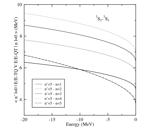
Figure 20: Contributions to $H^{eff}$ with explicit energy dependence, for $P$ defined by $\Lambda_{P}=8$ and $b=1.7$ fm. The upper left panel shows the diagonal “bare” kinetic energy term $\langle\alpha|T|\widetilde{\alpha}\rangle$ for the edge states $|\alpha\rangle=|n=5~{}l=0\rangle$, $|n=4~{}l=1\rangle$, and $|n=4~{}l=2\rangle$. The dots indicate the limiting values for very large and very small binding energies. The kinetic energy plotted is dimensionless, given in terms of $\hbar\omega/2$. The lower left panel gives the matrix elements of the bare potential $V$ between ${}^{3}S_{1}$ edge states, as a function of $E$. The upper right panel shows the evolution of the quantities $a_{LO}^{\prime}(E;n^{\prime},l^{\prime},n,l)/a_{LO}(n^{\prime},l^{\prime},n,l)$, $a_{NLO}^{\prime}(E;n^{\prime},l^{\prime},n,l)/a_{NLO}(n^{\prime},l^{\prime},n,l)$, etc., through N³LO for the diagonal matrix element with $|n=5~{}l=0\rangle.$ The general softening of such matrix elements is apparent, for small binding energy – repeated scattering by $T$ through high-energy oscillator states in $Q$ spreads the wave function and thus reduces the effects of the strong potential at short range. This effect is carried by the edge states, because their renormalization is affected by the missing long-range physics. See the text for further discussion.

The second $\kappa$-dependent term, the “bare” potential energy $\langle\widetilde{\alpha}(\kappa)|V|\widetilde{\beta}(\kappa)\rangle$, is displayed over the same range in the lower left panel of Fig. 20 for the five ${}^{3}S_{1}-{}^{3}S_{1}$ edge-state matrix elements. These matrix elements are again quite sensitive to $|E|$, varying by 2-3 MeV over the 20 MeV range displayed in the figure.

The third $\kappa$-dependence is the renormalization of the contact-gradient coefficients for edge states,

$$\langle n^{\prime}~{}l^{\prime}|{E\over E-TQ}\bar{O}{E\over E-QT}|n~{}l\rangle=\sum_{i,j=0}\widetilde{g}_{j}(-\kappa^{2};n^{\prime},l^{\prime})\widetilde{g}_{i}(-\kappa^{2};n,l)~{}\langle n^{\prime}+j~{}l^{\prime}|~{}\bar{O}~{}|n+i~{}l\rangle$$ (40)

Here $\bar{O}$ is fixed, while the explicit energy dependence carried by the $\widetilde{g}_{i}$ (i.e., the effects of the interplay between $QT$ and $QV$) is evaluated. The upper left panel in Fig. 20 gives the result for the diagonal edge-state matrix element, $|n^{\prime}~{}l^{\prime}\rangle=|n~{}l\rangle=|5~{}0\rangle$. As has been seen in other cases, the reduction due to the $QT-QV$ interplay is substantial throughout the illustrated 20 MeV range. Thus the large effects observed for the deuteron, a relatively weakly bound state, are in fact generic. But weakly bound states are more strongly affected, with the differences between the corrections for the double-edge states changing by a factor of nearly two between $|E|$=20 MeV and $|E|\sim 0$ MeV. The results for single-edge-state matrix elements are similar, but the changes are smaller by a factor of two.

In doing these calculations, some care is needed in going to the limit of very small binding energies. One can show for edge states

$$\widetilde{g}_{i}(-\kappa^{2};n,l)\stackrel{{\scriptstyle\mathrm{small}~{}\kappa}}{{\longrightarrow}}(-1)^{i}\left[{\Gamma(n+l+1/2)(n-1+i)!\over\Gamma(n+l+1/2+i)(n-1)!}\right]^{1/2}$$ (41)

If one uses this in Eq. (40) with $\kappa\equiv 0$, one finds that

$${\sum_{i=0}\widetilde{g}_{i}(0;n,l)\langle\vec{r}=0~{}|~{}n+i~{}l\rangle\over\langle\vec{r}=0~{}|~{}n~{}l\rangle}$$

oscillates (for an edge state) between 0 and 1, with every increment in $i$. However, a nonzero $\kappa^{2}$ acts as a convergence factor. If it is quite small, but not zero, the ratio then goes smoothly to 1/2. Consequently, as Fig. 20 shows, $a_{LO}^{\prime}/a_{LO}\rightarrow$ 1/4 in the limit of small, but nonzero $\kappa$.

The effects illustrated in Fig. 20 – the three effects explicitly governed by $\kappa$ – are associated with the coupling between $P$ and $Q$ generated by $T$. Because this operator connects states with $\Delta n=\pm 1$, there is no large energy scale associated with excitations. As the effects are encoded into a subset of the matrix elements, the overall scale of the $\kappa$ dependence on spectral properties is, at this point, still not obvious.

This leaves us with one remaining term that, qualitatively, seems quite different,

$$V{1\over E-QH}QV\leftrightarrow\{a_{LO}(|E|),~{}a_{NLO}(|E|),~{}a_{NNLO}(|E)|,~{}a_{N^{3}LO}(|E|),...\}.$$ (42)

Here the energy dependence is implicit, encoded in the parameters fitted to the lowest energy matrix elements of $H^{eff}$. The underlying potentials are dominated by strong, short-ranged potentials, much larger than nuclear binding energies. Thus the implicit ratio governing this energy dependence – $|E|$ vs. the strength of the hard-core potential – is a small parameter. For this reason one anticipates that the resulting energy dependence might be gentler than in the cases just explored.

After repeating the fitting procedure over a range of energies, one obtains the results shown in Fig. 21. Because the energy variation is quite small, results are provided only for the channels that contribute in low order, ${}^{1}S_{0}$, ${}^{3}S_{1}$, ${}^{1}P_{1}$ and ${}^{3}P_{J}$. The variation is very modest and regular, varying inversely with $|E|$ and well fit by the assumption (motivated by the form of $V(E-QH)^{-1}QV$)

$$a(E)={a(10MeV)\over 1+\alpha|E|}.$$

The variation is typically at the level of a few percent, over 20 MeV. The progression in the slopes within each channel, order by order, correspond to expectation: the lowest order terms, which account for the hardest part of the scattering in $Q$, have the weakest dependence on $|E|$. Comparisons between channels also reflect expectations. In the earlier discussion of naturalness, the rapid convergence in the ${}^{1}S_{0}$ channel, order by order, was consistent with very short range interactions in $Q$. Accordingly, $a_{LO}^{1S0}$ varies by just 0.72% over a 10 MeV interval, and $a_{NLO}^{1S0}$ by 1.10%. This channel contrasts with the ${}^{3}S_{1}$ channel, where convergence in the contact-gradient expansion is slower, consistent with somewhat longer range interactions in $Q$. For the ${}^{3}S_{1}$ case one finds 2.64% variations in $a_{LO}(^{3}S_{1})$ and 5.17% variations in $a_{NLO}(^{3}S_{1})$ per 10 MeV interval.

Are such variations of any numerical significance, compared to the explicit variations isolated in $\kappa$? That is, if one were to determine a HOBET interaction directly from bound-state properties of light nuclei, would the neglect of this implicit energy dependence lead to significant errors in binding energies? One can envision doing such a fit over bound-state data spanning $\sim$ 10 MeV, finding the couplings as a function of $|E|$, so that the error induced by using average energy-independent couplings $a_{LO}(|\bar{E}|)$ can be assessed. These errors would reflect variations in the matrix elements to which these couplings are fit, following the procedures previously described. Such a study showed that only two channels exhibited drifts $\Delta$ in excess of 15 keV over 10 MeV,

$$a_{LO}^{1S0}:\Delta\sim\pm 21\mathrm{~{}keV}~{}~{}~{}a_{LO}^{3S1}:\Delta\sim\pm 148\mathrm{~{}keV}~{}~{}~{}a_{NLO}^{3S1}:\Delta\sim\pm 32\mathrm{~{}keV}$$

One concludes that the ${}^{3}S_{1}$ channel is, by a large factor, the dominant source of implicit energy dependence in the HOBET interaction.

Figure 21: The calculated energy dependence of derived coefficients for the contact-gradient expansion are indicated by the markers, for the various $S-S$ and $P-P$ channels. Over a 10 MeV interval typical of bound-state nuclear spectra, variations are typically at the few percent level. The continuous lines represent simple linear fits, $a$(10 MeV)/$a(E)$ = 1 + $\alpha|E|$, to the results. The fit is generally excellent.

This allows one to do a more quantitative calculation that focuses on the most difficult channel (${}^{3}S_{1}$) and compares the relative sizes of the $\kappa$-dependent and implicit energy dependences, as reflected in changes in the matrix $H^{eff}(|E|)$. Thus this matrix is constructed at $|E|=10$ MeV and at $|E|\sim 0$ MeV (including the coupling to ${}^{3}D_{1}$), and changes in global quantities of that matrix over 10 MeV are examined: shifts in the first moment (the average eigenvalue) , the RMS shifts of levels relative to the first moment (related to the stability of level splittings), and eigenvalue overlaps. The four energy-dependent effects discussed here are separately turned on and off. Thus this exercise should provide a good test of the relative importance of these effects. The results are shown in Table 3.

Table 3: Spectral property variations in $H^{eff}(E)$ over 10 MeV

Term	Parameter	1st Moment Shift (MeV)	RMS Level Variation (MeV)	Wave Function Overlaps
$\langle\alpha|T|\widetilde{\beta}\rangle$	$\kappa$	2.554	1.107	95.75-99.74%
$\langle\widetilde{\alpha}|V|\widetilde{\beta}\rangle$	$\kappa$	0.272	0.901	99.35-99.82%
$\langle\widetilde{\alpha}|\bar{O}|\widetilde{\beta}\rangle$	$\kappa$	-0.239	0.957	99.51-99.99%
$\langle\alpha|\bar{O}(E)|\beta\rangle$	implicit	0.135	0.107	99.95-100%

Despite the selection of the worst channel, ${}^{3}S_{1}$, the implicit energy dependence is small, intrinsically and in comparison with the implicit energy dependence embedded in $\kappa$. The implicit dependence in the first moment – a quantity important to absolute binding energies – is 5% that of the explicit dependence in $\langle\alpha|T|\widetilde{\beta}\rangle$. The RMS shifts in levels relative the first moment are at the $\sim$ 1 MeV level for each of the implicit terms, but $\sim$ 100 keV for the implicit term. Eigenfunction overlaps show almost no dependence on the implicit term, exceeding 99.95% in all cases: variations 10-100 times larger arise from the analytical terms in $\kappa$.

Thus a simple representation of the HOBET effective interaction exists:

• The requirements for a state of fixed $|E|$ are a series of short-range coefficients and a single parameter $\kappa$ that governs long-range corrections residing in $Q$, including certain terms that couple $QV$ and $QT$. By various measures explored here, an N³LO expansion is accurate to about a few keV

• The $\kappa$ dependence found for a state of definite energy $|E|$ also captures almost all of the energy dependence resulting from varying $|E|$, the state-dependence in BH. Even in the most troublesome channel, calculations show that $\sim$ 95% of the energy dependence associated with changes in $|E|$ is explicit. It appears that neglect of the implicit energy dependence would induce errors of $\mathrel{\hbox to0.0pt{\lower 4.0pt\hbox{\hskip 1.0pt$\sim$}\hss}\raise 1.0pt\hbox{$<$}}$ 100 keV, for a spectrum spanning $\pm$ 10 MeV. This kind of error would be within the uncertainties of the best ab initio excited-state methods for light (p-shell) nuclei, such as Green’s function Monte Carlo argonne or large-basis no-core SM diagonalizations nocore .

• If better results are desired, the program described here can be extended to include the implicit energy dependence. The expansion around an average energy $E_{0}$

  $$V{1\over E-QH}QV=V\left[{1\over E_{0}-QH}-{1\over E_{0}-QH}(E-E_{0}){1\over E_{0}-QH}+\cdots\right]QV$$

  generates the correction linear in $E$ that is seen numerically. This second term is clearly quite small, explicitly suppressed by the ratio of scales discussed above. But, in any troublesome channel, the second term could be represented by contact-gradient operators of low order, with the contribution suppressed by an overall factor of $(E-E_{0})$.

V Discussion and Summary

One of the important motivations for trying to formulate an effective theory for nuclei in a harmonic oscillator basis is the prospect of incorporating into the approach some of the impressive numerical technology of approaches like the SM. Numerical techniques could be used to solve significant $P$-space problems, formulated in spaces, such as completed $N\hbar\omega$ bases, that preserve the problem’s translational invariance.

My collaborators and I made an initial effort to construct a HOBET some years ago, using a contact-gradient expansion modeled after EFT. We performed a shell-by-shell integration, in the spirit of a discrete renormalization group method, but encountered several abnormalities connected with the running of the coefficients of the expansion. Subsequent numerical work in which we studied individual matrix elements revealed the problems illustrated in Fig. 3. These problems – the difficulty of representing $Q$-space contributions that are both long range and short range – are not only important for HOBET, but also are responsible for the lack of convergence of perturbative expansions of the effective interaction. Fig. 1 provides one example. In other work luu we have shown that convergent expansions in the bare interaction (deuteron) or g-matrix (³He/³H) for $H^{eff}$ do exist, if the long-range part of this problem is first solved, as we have done here.

Thus the current paper returns to the problem of constructing a contact-gradient expansion for the effective interaction, taking into account what has been learned since the first, less successful effort. This paper introduces a form for that expansion that eliminates operator mixing, simplifying the fitting of coefficients and guaranteeing that coefficients determined in a given order remain fixed when higher-order terms are added. Thus the N³LO results presented here contain the results of all lower orders. The expansion is one in nodal quantum numbers, and is directly connected with traditional Talmi integral expansions, generalized for nonlocal interactions.

Convergence does vary from channel to channel, but in each channel the order-by-order convergence is very regular. Each new order brings down the scale $\Lambda$ at which deviations appear, and in each new order the Lepage plot steepens, showing that the omitted physics does have the expected dependence on higher-order polynomials in $(n^{\prime},n)$. The channel-by-channel variations in convergence reflect similar behavior seen in EFT approaches, where the need for alternative power counting schemes has been noted to account for this behavior. From a practical standpoint, however, the N³LO results are effectively exact: in the most important difficult channel, ${}^{3}S_{1}$, measures of the quality of the matrix $H^{eff}$ yielded results on the order of (1-3) keV.

The summation done over $QT$ yields a simple result, but still one that is quite remarkable in that long-range physics is governed by a single parameter $\kappa$, that depends on the ratio of $|E|$ and $\hbar\omega$. Despite all of the attractive analytic properties of the HO as a basis for bound states, its unphysical binding at large $r$ has been viewed as a shortcoming. But the ladder properties of the HO in fact allow an exact summation of $QT$. It seems unlikely that any other bound-state basis would allow the coupling of $P$ and $Q$ by $T$ to be exactly removed. That is, the HO basis may be the only one that allows the long-range physics in $Q$ to be fully isolated, and thus subtracted systematically. In this sense it may be the optimal basis for correctly describing the asymptotic behavior of the wave function. Note, in particular, that the right answer is not going to result from using “improved” single-particle bases: $\kappa$ depends of $|E|$, not on single-particle energies of some mean field.

The effects associated with $\kappa$ are large, typically shifting edge-state matrix elements by several MeV, and altering spectral measures, like the first energy moment of $H^{eff}$, by similar amounts. This dependence, if not isolated, destroys the systematic order-by-order improvement important to HOBET, as Fig. 3 clearly illustrates.

The explicit energy dependence captured in $\kappa$ accounts for almost all of the energy dependence of $H^{eff}(|E|)$. In more complicated calculations this dependence, in the BH formulation used here, generates the state-dependence that allows ET wave functions to have the proper relationship to the exact wave functions, namely that the former are the $P$-space restrictions of the latter. While in principle additional energy dependence important to this evolution resides in $V(E-QH)^{-1}QV$ and thus in the coefficients of the contact-gradient expansion, in practice this residual implicit energy dependence was found to be very weak. This dependence was examined channel by channel, and its impact on global properties of $H^{eff}(|E|)$ was determined for the most troublesome channel, ${}^{3}S_{1}$. Even in this channel, the impact of the remaining implicit energy dependence on $H^{eff}(|E|)$ spectral properties such as the first moment, eigenvalue spacing, and eigenvalue overlaps, was found to be quite small compared to the explicit dependence isolated in $\kappa$. This is physically very reasonable: $QT$ generates nearest-shell couplings between $P$ and $Q$, so that excitation scales are comparable to typical nuclear binding energies. Thus this physics, extracted and expressed as a function of $\kappa$, should be sensitive to binding energies. In contrast, $V(E-QH)^{-1}QV$ involves large scales associated with the hard core, and thus should be relatively insensitive to variations in $|E|$. In the ${}^{3}S_{1}$ channel, the explicit dependence captured in $\kappa$ is about 20 times larger than the implicit energy dependence buried in the contact-gradient coefficients. Numerically, the latter could cause drifts on the order of 100 keV over 10 MeV intervals. Thus, to an excellent approximation, one could treat these coefficients as constants in fitting the properties of low-lying spectra. Alternatively, the HOBET procedure for accounting for this implicit energy dependence has been described, and could be used in any troublesome channel.

The weakness of the implicit energy dependence will certainly simplify future HOBET efforts to determine $H^{eff}(E,b,\Lambda_{P})$ directly from data (rather than from an NN potential like $v_{18}$). Indeed, such an effort will be the next step in the program. The approach outlined here is an attractive starting point, as it can be shown that the states $|\widetilde{\alpha}(\kappa)\rangle$ become asymptotic plane-wave states, when $E$ is positive. Thus the formalism relates bound and continuum states through a common set of strong-interaction coefficients operating in a finite orthogonal basis.

The relationship between current work and some more traditional treatments of the $H^{eff}$ for model-based approaches, like the SM, should be mentioned. Efforts like those of Kuo and Brown are often based on the division $H=H_{0}+(V-V_{0})$, where $H_{0}$ is the HO Hamiltonian kuobrown . Such a division would allow the same BH reorganization done here: $QT$ and $Q(H_{0}-V_{0})$ are clearly equivalent. But in practice terms are, instead, organized in perturbation theory according to $H_{0}$, i.e., so that Green’s functions involve single-particle energies. This would co-mingle the long- and short-range physics is a very complicated way. In addition, often the definitions of $Q$ and $P$ used in numerical calculations are not those of the HO: instead, a plane-wave momentum cut is often used, which simplifies the calculations but introduces uncontrolled errors. Either this approximation (plane waves are diagonal in $T$) or the use of perturbation theory (because of the co-mingling) would appear to make it impossible to separate long- and short-range physics correctly, as has been done here.

Another example is $V_{low~{}k}$, in which a softer two-nucleon potential is derived by integration over high-momentum states achim . This is a simpler description of $Q$ than arises in bound-state bases problems, like those considered here: the division between $P$ and $Q$ is a specified momentum, and $T$ is diagonal. There would be no analog of the $\kappa$-dependence found in HOBET. However, HOBET and $V_{low~{}k}$ may have an interesting relationship. Effective operators for HOBET and for EFT approaches (which also employ a momentum cutoff) agree in lowest contributing order. When there are differences in higher order, it would seem that these differences must vanish by taking the appropriate limit, namely the limit of the HOBET $Q(b,\Lambda_{P})$ where $b\rightarrow\infty$ while $\Lambda_{P}/b$ is kept fixed. This keeps the average $\langle p^{2}\rangle$ of the last included shell fixed, while forcing the number of shells to infinity and the shell splitting to zero. Numerically it would be sufficient to approach this limit, so that $Q$ resembles the plane-wave limit over a distance characteristic of the nuclear size. It is a reasonable conjecture that $V_{low~{}k}$ would emerge from such a limit of the HOBET $H^{eff}(b,\Lambda_{P})$. It would follow that all $\kappa$ dependence should vanish in that limit. It would be interesting to try to verify these conjectures in future work, and to study the evolution of the HOBET effective interaction coefficients as this limit is taken

The state-dependence of effective interactions is sometimes treated in nuclear physics by the method of Lee and Suzuki. One form of Lee-Suzuki produces a Hermitian energy-independent interaction. While it is always possible to find such an $H$ to reproduce eigenvalues, it is clear that basic wave function requirements of an effective theory – that the included wave functions correspond to restrictions of the true wave functions to $P$ – are not consistent with such an $H$.

Another form produces an energy-independent but nonHermitian $H$. This can be done consistently in an effective theory. However, the results presented here make it difficult to motivate such a transformation. It appears that the state-dependence is almost entirely attributable to the interplay between $QT$ and $QV$, removed here analytically in terms of a function of one parameter $\kappa$, which relates the bound-state momentum scale (in $\hbar\omega$) to a state’s energy. There is no obvious benefit in obscuring this simple dependence in a numerical transformation of the potential, given that the Lee-Suzuki method is not easy to implement. The physics is far more transparent in the BH formulation, and the self-consistency required in BH makes the use of an energy-dependent potential as easy as an energy-independent one. More to the point, the necessary $\kappa$ dependence is already encoded in the potential for a single state of definite energy $|E|$ – thus no additional complexity is posed by the state-dependence of the potential.

I thank Tom Luu and Martin Savage for helpful discussions. This work was supported in part by the Office of Nuclear Physics and SciDAC, US Department of Energy.

VI References

VII APPENDIX: Effective Interaction Matrix Elements

This appendix provides details on the evaluation of the modified HO states

$${E\over E-QT}|n~{}l\rangle.$$ (A-1)

for nodal quantum numbers $n=1,2,3,...$, and for corresponding contact-gradient effective interaction matrix elements between such states. Closed-form expressions allow these matrix elements to be evaluated quickly to any order. Here two alternative evaluations are provided, one based on a harmonic oscillator expansion and one on the free Green’s function.

Harmonic Oscillator Expansion: The harmonic oscillator Green’s function expansion is

$${E\over E-QT}|n~{}l\rangle=\sum_{i=0}^{\infty}\widetilde{g}_{i}(-\kappa^{2};n,l)|n+i~{}l\rangle$$ (A-2)

where the $\widetilde{g}_{i}$ are determined by a set of continued fractions generated from the ladder properties of the operator $QT$. In practice the sum can be truncated: numerical convergence is discussed below, in comparison with the Green’s function approach. While this paper focuses on the simple example of the deuteron, the approach is more general : the relationship between the relative kinetic energy and the three-dimensional harmonic oscillator can be extended to the n-dimensional harmonic oscillator, with the hyperspherical harmonics replacing the spherical harmonics as eigenfunctions of the kinetic energy. The corresponding ladder properties for the harmonic oscillator in hyperspherical coordinates are known hyper : this is the essential requirement for the expansion.

As discussed in the text, it is convenient to modify the usual contact-gradient expansion, to remove operator mixing and create an expansion in nodal quantum numbers. Each term $O$ in the usual contact-gradient expansion is replaced by

$$O\rightarrow\bar{O}\equiv e^{r^{2}/2}Oe^{r^{2}/2}$$ (A-3)

where $r$ is the dimensionless Jacobi coordinate $|\vec{r}_{1}-\vec{r}_{2}|/(b\sqrt{2})$. Gradients appearing in $O$ are also defined in terms of this dimensionless coordinate.

In each partial wave the lowest contributing operators are based on gradients, maximally coupled, acting on wave functions, with the result evaluated at $\vec{r}=0$. For example, for $S$, $P$, and $D$ states

$$e^{r^{2}/2}R_{nl}(r)Y_{l0}(\Omega_{r})\big{|}_{\vec{r}=0} = \delta_{l0}{1\over\pi}\left[{2\Gamma(n+1/2)\over(n-1)!}\right]^{1/2}$$

$$\overrightarrow{\nabla}_{10}~{}e^{r^{2}/2}R_{nl}(r)Y_{l0}(\Omega_{r})\big{|}_{\vec{r}=0} = \delta_{l1}\sqrt{{2(2n+1)\over 3}}R_{n0}(r)Y_{00}(\Omega_{r})\big{|}_{r=0}=\delta_{l1}~{}2\left[{1!\over 3!!}\right]^{1/2}{1\over\pi}\left[{2~{}\Gamma[n+3/2]\over(n-1)!}\right]^{1/2}$$

$$(\overrightarrow{\nabla}\otimes\vec{\nabla})_{20}e^{r^{2}/2}R_{nl}(r)Y_{l0}(\Omega_{r})\big{|}_{\vec{r}=0} = \delta_{l2}\sqrt{{8(2n+1)(2n+3)\over 15}}R_{n0}(r)Y_{00}(\Omega_{r})\big{|}_{\vec{r}=0}=\delta_{l2}~{}2^{2}\left[{2!\over 5!!}\right]^{1/2}{1\over\pi}\left[{2~{}\Gamma[n+5/2]\over(n-1)!}\right]^{1/2}$$

As the gradients are maximally coupled, all coupling schemes are equivalent. If one defines by $(\overrightarrow{\nabla}^{q})_{q0}$ the expressions with $q$ gradients maximally coupled, the results of Eq. (LABEL:eq:ex) are examples of the more general formula

$$({\overrightarrow{\nabla}}^{q})_{q0}~{}e^{r^{2}/2}R_{nl}(r)Y_{l0}(\Omega_{r})\big{|}_{\vec{r}=0}=\delta_{lq}~{}2^{l}\left[{l!\over(2l+1)!!}\right]^{1/2}{1\over\pi}\left[{2~{}\Gamma[n+l+1/2]\over(n-1)!}\right]^{1/2}.$$ (A-5)

A form of this equation that will be used below is

$$(\overrightarrow{\nabla}^{q})_{q0}~{}e^{r^{2}/2}R_{n-p~{}l}(r)Y_{l0}(\Omega_{r})\big{|}_{\vec{r}=0}=\delta_{lq}~{}2^{l}\left[{l!\over(2l+1)!!}\right]^{1/2}{1\over\pi}\left[{2~{}\Gamma[n+l+1/2-p]\over(n-1-p)!}\right]^{1/2}$$

$$~{}~{}~{}~{}~{}~{}=\left[{(n-1)!~{}\Gamma[n+l+1/2-p]\over(n-1-p)!~{}\Gamma[n+l+1/2]}\right]^{1/2}\delta_{lq}~{}2^{l}\left[{l!\over(2l+1)!!}\right]^{1/2}{1\over\pi}\left[{2~{}\Gamma[n+l+1/2]\over(n-1)!}\right]^{1/2}$$ (A-6)

Contact-gradient operators beyond the lowest contributing order involve $\overrightarrow{\nabla}^{2}$ acting on harmonic oscillator wave functions. One can quickly verify

$$\overrightarrow{\nabla}^{2}e^{r^{2}/2}R_{nl}(r)Y_{lm}(\Omega_{r})=-4\sqrt{(n-1)(n+l-1/2)}e^{r^{2}/2}R_{n-1~{}l}(r)Y_{lm}(\Omega_{r})$$ (A-7)

so that

$$(\overrightarrow{\nabla}^{2})^{p}e^{r^{2}/2}R_{nl}(r)Y_{lm}(\Omega_{r})=(-4)^{p}\left[{(n-1)!~{}\Gamma[n+l+1/2]\over(n-1-p)!~{}\Gamma[n+l+1/2-p]}\right]^{1/2}e^{r^{2}/2}R_{n-p~{}l}(r)Y_{lm}(\Omega_{r}).$$ (A-8)

Thus by first using Eq. (A-8) and then applying Eq. (A-6), one finds the general expression for a contact-gradient operator of arbitrary order acting on a harmonic oscillator state

$$(\overrightarrow{\nabla}^{2})^{p}(\overrightarrow{\nabla}^{q})_{q0}e^{r^{2}/2}R_{nl}(r)Y_{lm}(\Omega_{r})\big{|}_{\vec{r}=0}=\delta_{lq}~{}(-4)^{p}{(n-1)!\over(n-1-p)!}\left(2^{l}\left[{l!\over(2l+1)!!}\right]^{1/2}{1\over\pi}\left[{2~{}\Gamma[n+l+1/2]\over(n-1)!}\right]^{1/2}\right)$$ (A-9)

Equation (A-9) defines the needed matrix elements, evaluated below for each partial-wave channel contributing through N³LO. [Note that if one wanted to write a potential, as opposed to partial-wave matrix elements of that potential that are given here, suitable projection operators could be inserted as needed. For example, the $l=0$ triplet and singlet channels could be distinguished by introducing the projection operators $P(^{3}S_{1})=(3+\vec{\sigma}_{1}\cdot\vec{\sigma}_{2})/4=\vec{S}^{2}/2$ and $(1-\vec{\sigma}_{1}\cdot\vec{\sigma}_{2})/4=1-\vec{S}^{2}/2$, respectively; the three triplet $l=1$ channels could be distinguished from the singlet $l=1$ channel and from each other by the projectors

$$P(^{3}P_{0}) = {(-1+(\vec{l}\cdot\vec{S})^{2})~{}\vec{S}^{2}\over 6}$$

$$P(^{3}P_{1}) = {(2-\vec{l}\cdot\vec{S}-(\vec{l}\cdot\vec{S})^{2})~{}\vec{S}^{2}\over 4}$$

$$P(^{3}P_{2}) = {(2+3~{}\vec{l}\cdot\vec{S}+(\vec{l}\cdot\vec{S})^{2})~{}\vec{S}^{2}\over 12}$$ (A-10)

and so on.] The matrix elements of Table 1, which all are scalar products of spin-spatial tensor operators, are of two types. One is diagonal in $l$, where $O=\overleftarrow{O}^{L}_{l}\cdot\delta(\vec{r})~{}\overrightarrow{O}^{R}_{l}$, with $\overleftarrow{O}^{L}_{l}$ and $\overrightarrow{O}^{R}_{l}$ spatial tensors. In this case

$$\langle n^{\prime}(lS)JMTM_{T}|O|n(lS)JMTM_{T}\rangle=\langle n^{\prime}lm_{l}=0|\overleftarrow{O}^{L}_{l0}~{}\delta({\vec{r}})~{}\overrightarrow{O}^{R}_{l0}|nlm_{l}=0\rangle$$ (A-11)

The second type of operator, $O=\overleftarrow{O}^{L}_{l}\cdot\delta(\vec{r})~{}[\overrightarrow{O}^{R}_{l+2}\otimes[\sigma(1)\otimes\sigma(2)]_{2}]_{l}$, enters for the off-diagonal triplet $S-D$,$P-F$, and $D-G$ cases,

$$\langle n^{\prime}(lS=1)J=l+1~{}MTM_{T}|O|n(l+2~{}S=1)J=l+1~{}MTM_{T}\rangle=$$

$$~{}~{}~{}~{}~{}~{}2\sqrt{{2l+1\over 2l+3}}~{}\langle n^{\prime}~{}l~{}m_{l}=0|\overleftarrow{O}^{L}_{l~{}0}~{}\delta(\vec{r})~{}\overrightarrow{O}^{R}_{l+2~{}0}|n~{}{l+2}~{}m_{l}=0\rangle$$ (A-12)

As both of these expressions reduce the matrix element to a product of terms like Eq. (A-9), the needed N³LO matrix elements follow directly. For the ${}^{3}S_{1}\leftrightarrow{}^{3}S_{1}$ or ${}^{1}S_{0}\leftrightarrow{}^{1}S_{0}$ channels,

$$\langle n^{\prime}(l=0S)JMTM_{T}|e^{r^{2}/2}\biggl{[}a_{LO}^{3S1}\delta(\vec{r})+a_{NLO}^{3S1}(\overleftarrow{\nabla}^{2}\delta(\vec{r})+\delta(\vec{r})\overrightarrow{\nabla}^{2})+a_{NNLO}^{3S1,22}\overleftarrow{\nabla}^{2}\delta(\vec{r})\overrightarrow{\nabla}^{2}+a_{NNLO}^{3S1,40}(\overleftarrow{\nabla}^{4}\delta(\vec{r})+\delta(\vec{r})\overrightarrow{\nabla}^{4})$$ (A-13)

$$+a_{N^{3}LO}^{3S1,42}(\overleftarrow{\nabla}^{4}\delta(\vec{r})\overrightarrow{\nabla}^{2}+\overleftarrow{\nabla}^{2}\delta(\vec{r})\overrightarrow{\nabla}^{4})+a_{N^{3}LO}^{3S1,60}(\overleftarrow{\nabla}^{6}\delta(\vec{r})+\delta(\vec{r})\overrightarrow{\nabla}^{6})\biggr{]}e^{r^{2}/2}|n(l=0S)JMTM_{T}\rangle=\hskip 86.72377pt$$

$$\hskip 21.68121pt{2\over\pi^{2}}\left[{\Gamma[n^{\prime}+1/2]\Gamma[n+1/2]\over(n^{\prime}-1)!(n-1)!}\right]^{1/2}~{}\biggl{(}a_{LO}^{3S1}-4((n^{\prime}-1)+(n-1))a_{NLO}^{3S1}+$$

$$\hskip 21.68121pt+16\bigl{[}(n^{\prime}-1)(n-1)a_{NNLO}^{3S1,22}+((n^{\prime}-1)(n^{\prime}-2)+(n-1)(n-2))a_{NNLO}^{3S1,40}\bigr{]}-64\bigl{[}((n^{\prime}-1)(n^{\prime}-2)(n-1)+$$

$$\hskip 21.68121pt(n^{\prime}-1)(n-1)(n-2))a_{N3LO}^{3S1,42}+((n^{\prime}-1)(n^{\prime}-2)(n^{\prime}-3)+(n-1)(n-2)(n-3))a_{N3LO}^{3S1,60}\bigr{]}\biggr{)};$$

For the ${}^{3}S_{1}\leftrightarrow{}^{3}D_{1}$ channel, recalling $\overrightarrow{D}^{0}_{0}\equiv((\overrightarrow{\nabla}\otimes\overrightarrow{\nabla})_{2}\otimes(\sigma(1)\otimes\sigma(2))_{2})_{00}$,

$$\langle n^{\prime}(l=0S=1)J=1MTM_{T}|e^{r^{2}/2}\biggl{[}a_{NLO}^{SD}(\delta(\vec{r})\overrightarrow{D}^{0}_{0}+\overleftarrow{D}^{0}_{0}\delta(\vec{r}))+a_{NNLO}^{SD,22}(\overleftarrow{\nabla}^{2}\delta(\vec{r})\overrightarrow{D}^{0}_{0}+\overleftarrow{D}^{0}_{0}\delta(\vec{r})\overrightarrow{\nabla}^{2})+$$ (A-14)

$$a_{NNLO}^{SD,04}(\delta(\vec{r})\overrightarrow{\nabla}^{2}\overrightarrow{D}^{0}_{0}+\overleftarrow{D}^{0}_{0}\overleftarrow{\nabla}^{2}\delta(\vec{r}))+a_{N^{3}LO}^{SD,42}(\overleftarrow{\nabla}^{4}\delta(\vec{r})\overrightarrow{D}^{0}_{0}+\overleftarrow{D}^{0}_{0}\delta(\vec{r})\overrightarrow{\nabla}^{4})+$$

$$a_{N^{3}LO}^{SD,24}(\overleftarrow{\nabla}^{2}\delta(\vec{r})\overrightarrow{\nabla}^{2}\overrightarrow{D}_{0}^{0}+\overleftarrow{D}^{0}_{0}\overleftarrow{\nabla}^{2}\delta(\vec{r})\overrightarrow{\nabla}^{2})+a_{N^{3}LO}^{SD,06}(\delta(\vec{r})\overrightarrow{\nabla}^{4}\overrightarrow{D}_{0}^{0}+\overleftarrow{D}^{0}_{0}\overleftarrow{\nabla}^{4}\delta(\vec{r}))\biggr{]}e^{r^{2}/2}|n(l=2S=1)J=1MTM_{T}\rangle=$$

$$\hskip 21.68121pt{8\over 15}\sqrt{10}{2\over\pi^{2}}\left[{\Gamma[n^{\prime}+1/2]\Gamma[n+5/2]\over(n^{\prime}-1)!(n-1)!}\right]^{1/2}\biggl{(}a_{NLO}^{SD}-4\bigl{[}(n^{\prime}-1)a_{NNLO}^{SD,22}+(n-1)a_{NNLO}^{SD,04}\bigr{]}+$$

$$\hskip 21.68121pt16\bigl{[}(n^{\prime}-1)(n^{\prime}-2)a_{N^{3}LO}^{SD,42}+(n^{\prime}-1)(n-1)a_{N^{3}LO}^{SD,24}+(n-1)(n-2)a_{N^{3}LO}^{SD,06}\bigr{]}\biggr{)};$$

For the ${}^{1}D_{2}\leftrightarrow{}^{1}D_{2}$ or ${}^{3}D_{J}\leftrightarrow{}^{3}D_{J}$ channels, recalling $\overrightarrow{D}^{2}_{M}\equiv(\overrightarrow{\nabla}\otimes\overrightarrow{\nabla})_{2M}$,

$$\langle n^{\prime}(l=2S)J=1MTM_{T}|e^{r^{2}/2}\biggl{[}a_{NNLO}^{1D2}\overleftarrow{D}^{2}\cdot\delta(\vec{r})\overrightarrow{D}^{2}+a_{N^{3}LO}^{1D2}(\overleftarrow{D}^{2}\overleftarrow{\nabla}^{2}\cdot\delta(\vec{r})\overrightarrow{D}^{2}+\overleftarrow{D}^{2}\cdot\delta(\vec{r})\overrightarrow{\nabla}^{2}\overrightarrow{D}^{2})\biggr{]}e^{r^{2}/2}$$ (A-15)

$$|n(l=2S)J=1MTM_{T}\rangle={32\over 15}{2\over\pi^{2}}\left[{\Gamma[n^{\prime}+5/2]\Gamma[n+5/2]\over(n^{\prime}-1)!(n-1)!}\right]^{1/2}\biggl{(}a_{NNLO}^{1D2}-4\bigl{[}(n^{\prime}-1)+(n-1)\bigr{]}a_{N^{3}LO}^{1D2}\biggr{)};\hskip 38.30301pt$$

For the ${}^{3}D_{3}\leftrightarrow{}^{3}G_{3}$ channel, recalling $\overrightarrow{G}^{2}_{M}\equiv\left[((\overrightarrow{\nabla}\otimes\overrightarrow{\nabla})_{2}\otimes(\overrightarrow{\nabla}\otimes\overrightarrow{\nabla})_{2})_{4}\otimes(\sigma(1)\otimes\sigma(2))_{2}\right]_{2M}$,

$$\langle n^{\prime}(l=2S=1)J=3MTM_{T}|e^{r^{2}/2}a_{N^{3}LO}^{DF}(\overleftarrow{D}^{2}\cdot\delta(\vec{r})\overrightarrow{G}^{2}+\overleftarrow{G}^{2}\cdot\delta(\vec{r~{}~{}})\overrightarrow{D}^{2})e^{r^{2}/2}|n(l=4S=1)J=3MTM_{T}\rangle=$$ (A-16)

$$\hskip 21.68121pt{512\over 315}\sqrt{15}{2\over\pi^{2}}\left[{\Gamma[n^{\prime}+5/2]\Gamma[n+9/2]\over(n^{\prime}-1)!(n-1)!}\right]^{1/2}a_{N^{3}LO}^{DF};\hskip 260.17244pt$$

For the ${}^{1}P_{1}\leftrightarrow{}^{1}P_{1}$ or ${}^{3}P_{J}\leftrightarrow{}^{3}P_{J}$ channels,

$$\langle n^{\prime}(l=1S)JMTM_{T}|e^{r^{2}/2}\biggl{[}a_{NLO}^{1P1}\overleftarrow{\nabla}\cdot\delta(\vec{r})\overrightarrow{\nabla}+a_{NNLO}^{1P1}(\overleftarrow{\nabla}\overleftarrow{\nabla}^{2}\cdot\delta(\vec{r})\overrightarrow{\nabla}+\overleftarrow{\nabla}\cdot\delta(\vec{r})\overrightarrow{\nabla}^{2}\overrightarrow{\nabla})+$$ (A-17)

$$a_{N^{3}LO}^{1P1,33}\overleftarrow{\nabla}\overleftarrow{\nabla}^{2}\cdot\delta(\vec{r})\overrightarrow{\nabla}^{2}\overrightarrow{\nabla}+a_{N^{3}LO}^{1P1,51}(\overleftarrow{\nabla}\overleftarrow{\nabla}^{4}\cdot\delta(\vec{r})\overrightarrow{\nabla}+\overleftarrow{\nabla}\cdot\delta(\vec{r})\overrightarrow{\nabla}^{4}\overrightarrow{\nabla})\biggr{]}e^{r^{2}/2}|n(l=1S)JMTM_{T}\rangle=$$

$$\hskip 21.68121pt{4\over 3}{2\over\pi^{2}}\left[{\Gamma[n^{\prime}+3/2]\Gamma[n+3/2]\over(n^{\prime}-1)!(n-1)!}\right]^{1/2}~{}\biggl{(}a_{NLO}^{1P1}-4((n^{\prime}-1)+(n-1))a_{NNLO}^{1P1}+\hskip 137.31255pt$$

$$\hskip 21.68121pt+16\bigl{[}(n^{\prime}-1)(n-1)a_{N^{3}LO}^{1P1,33}+((n^{\prime}-1)(n^{\prime}-2)+(n-1)(n-2))a_{N^{3}LO}^{1P1,51}\bigr{]}\biggr{)};$$

For the ${}^{3}P_{2}\leftrightarrow{}^{3}F_{2}$ channel, recalling $\overrightarrow{F}^{1}_{M}\equiv\left[(\overrightarrow{\nabla}\otimes(\overrightarrow{\nabla}\otimes\overrightarrow{\nabla})_{2})_{3}\otimes(\sigma(1)\otimes\sigma(2))_{2}\right]_{1M}$,

$$\langle n^{\prime}(l=1S=1)J=2MTM_{T}|e^{r^{2}/2}\biggl{[}a_{NNLO}^{PF}(\overleftarrow{\nabla}\cdot\delta(\vec{r})\overrightarrow{F}^{1}+\overleftarrow{F}^{1}\cdot\delta(\vec{r})\overrightarrow{\nabla})+a_{N^{3}LO}^{PF,33}(\overleftarrow{\nabla}\overleftarrow{\nabla}^{2}\cdot\delta(\vec{r})\overrightarrow{F}^{1}+$$ (A-18)

$$\overleftarrow{F}^{1}\cdot\delta(\vec{r})\overrightarrow{\nabla}^{2}\overrightarrow{\nabla})+a_{N^{3}LO}^{PF,15}(\overleftarrow{\nabla}\cdot\delta(\vec{r})\overrightarrow{\nabla}^{2}\overrightarrow{F}^{1}+\overleftarrow{F}^{1}\overleftarrow{\nabla}^{2}\cdot\delta(\vec{r})\overrightarrow{\nabla})\biggr{]}e^{r^{2}/2}|n(l=3S=1)J=2MTM_{T}\rangle=$$

$$\hskip 21.68121pt{32\over 35}\sqrt{14}{2\over\pi^{2}}\left[{\Gamma[n^{\prime}+3/2]\Gamma[n+7/2]\over(n^{\prime}-1)!(n-1)!}\right]^{1/2}~{}\biggl{(}a_{NNLO}^{PF}-4\bigl{[}(n^{\prime}-1)a_{N^{3}LO}^{PF,33}+(n-1)a_{N^{3}LO}^{PF,15}\bigr{]}\biggr{)};\hskip 93.95122pt$$

And finally, for the ${}^{1}F_{3}\leftrightarrow{}^{1}F_{3}$ or ${}^{3}F_{J}\leftrightarrow{}^{3}F_{J}$ channels, recalling $\overrightarrow{F}^{3}_{M}\equiv(\overrightarrow{\nabla}\otimes(\overrightarrow{\nabla}\otimes\overrightarrow{\nabla})_{2})_{3M}$,

$$\langle n^{\prime}(l=3S)JMTM_{T}|e^{r^{2}/2}\biggl{[}a_{N^{3}LO}^{1F3}\overleftarrow{F}^{3}\cdot\delta(\vec{r})\overrightarrow{F}^{3}\biggr{]}e^{r^{2}/2}|n(l=3S)JMTM_{T}\rangle$$ (A-19)

$$\hskip 21.68121pt{128\over 35}{2\over\pi^{2}}\left[{\Gamma[n^{\prime}+7/2]\Gamma[n+7/2]\over(n^{\prime}-1)!(n-1)!}\right]^{1/2}~{}a_{N^{3}LO}^{PF}.\hskip 281.85255pt$$

In each case the general matrix element of the effective interaction, for edge amd nonedge states, can then be expanded in terms of Eqs. (A-13-A-19),

$$\langle n^{\prime}(l^{\prime}S)JMTM_{T}|{E\over E-TQ}\bar{O}{E\over E-QT}|n(lS)JMTM_{T}\rangle=$$ (A-20)

$$\hskip 21.68121pt\sum_{i,j=0}\widetilde{g}_{j}(-\kappa^{2};n^{\prime},l^{\prime})\widetilde{g}_{i}(-\kappa^{2};n,l)~{}\langle n^{\prime}+j~{}(l^{\prime}S)JMTM_{T}|~{}\bar{O}~{}|n+i~{}(lS)JMTM_{T}\rangle~{}.\hskip 108.405pt$$

Free Green’s Function Results: An equivalent set of results can be derived by making use of Eq. (36)

$$\langle\vec{r}|{E\over E-QT}|n~{}l~{}m_{l}\rangle\equiv\langle\vec{r}|\widetilde{\alpha}_{nlm_{l}}\rangle=-Y_{lm_{l}}(\Omega_{r})\biggl{[}{1\over\sqrt{r}}~{}I_{l+1/2}(\kappa r)\int_{r}^{\infty}{r^{\prime}}^{2}dr^{\prime}{1\over\sqrt{r^{\prime}}}K_{l+1/2}(\kappa r^{\prime})~{}\langle\vec{r}^{~{}\prime}|\alpha_{nlm_{l}}>$$ (A-21)

$$\hskip 21.68121pt+{1\over\sqrt{r}}~{}K_{l+1/2}(\kappa r)\int_{0}^{r}{r^{\prime}}^{2}dr^{\prime}{1\over\sqrt{r^{\prime}}}I_{l+1/2}(\kappa r^{\prime})~{}\langle\vec{r}^{~{}\prime}|\alpha_{nlm_{l}}>\equiv\widetilde{R}^{\alpha}_{nl}(r)Y_{lm_{l}}(\Omega_{r})\hskip 144.54pt$$

where the source term in the Green’s function is

$$|\alpha_{nlm_{l}}\rangle\equiv\bigl{[}-\kappa^{2}-(2n+l-1/2)-\widetilde{g}_{1}(-\kappa^{2};n,l)\sqrt{n(n+l+1/2)}~{}\bigr{]}|nlm_{l}>-\sqrt{(n-1)(n+l-1/2)}|n-1lm_{l}\rangle$$ (A-22)

$$\hskip 21.68121pt-\sqrt{n(n+l+1/2)}P[n+1,l]|n+1lm_{l}\rangle~{}.\hskip 296.30743pt$$

The inclusion of the last term makes this equation valid for non-edge as well as edge states: $P[n+1,l]=1$ if and only if $|n+1~{}l\rangle$ belongs to $P$. The reproduction of simple HO nonedge states is a helpful numerical check. Here $\langle\vec{r}|\alpha_{nlm_{l}}\rangle\equiv R^{\alpha}_{nl}(r)Y_{lm_{l}}(\Omega_{r})$.

The first task is to evaluate $(\overrightarrow{\nabla}^{2})^{p}e^{r^{2}/2}$ on this wave function. The inclusion of $e^{r^{2}/2}$ – which eliminates mixing among HO states and simplifies other HO expressions – is a bit of an annoyance in the Green’s function case, generating a series of surface terms. One finds the generic result, analogous to Eq. (A-7),

$$(\overrightarrow{\nabla}^{2})^{p}~{}e^{r^{2}/2}\widetilde{R}^{\alpha}_{nl}(r)Y_{lm_{l}}(\Omega_{r})=e^{r^{2}/2}Y_{lm_{l}}(\Omega_{r})\times$$ (A-23)

$$\hskip 21.68121pt\biggl{\{}\biggl{[}-f_{I}^{p}(\kappa^{2},r^{2}){1\over\sqrt{r}}I_{l+1/2}(\kappa r)-f_{I^{\prime}}^{p}(\kappa^{2},r^{2})2r{d\over dr}\biggl{(}({1\over\sqrt{r}}I_{l+1/2}(\kappa r)\biggr{)}\biggr{]}\int_{r}^{\infty}x^{2}dx{1\over\sqrt{x}}K_{l+1/2}(\kappa x)R^{\alpha}_{nl}(x)$$

$$\hskip 21.68121pt+\biggl{[}-f_{K}^{p}(\kappa^{2},r^{2}){1\over\sqrt{r}}K_{l+1/2}(\kappa r)-f_{K^{\prime}}^{p}(\kappa^{2},r^{2})2r{d\over dr}\biggl{(}({1\over\sqrt{r}}K_{l+1/2}(\kappa r)\biggr{)}\biggr{]}\int_{0}^{r}x^{2}dx{1\over\sqrt{x}}I_{l+1/2}(\kappa x)R^{\alpha}_{nl}(x)\biggr{\}}\hskip 36.135pt$$

$$\hskip 28.90755pt+f_{\alpha}^{p}(\kappa^{2},r^{2})e^{r^{2}/2}R^{\alpha}_{nl}(r)Y_{lm_{l}}(\Omega_{r})+f_{\alpha^{\prime}}^{p}(\kappa^{2},r^{2})2r{d\over dr}\bigl{(}e^{r^{2}/2}R^{\alpha}_{nl}(r)Y_{lm_{l}}(\Omega_{r})\bigr{)}$$

$$\hskip 28.90755pt+f_{\alpha^{\prime\prime}}^{p}(\kappa^{2},r^{2})\overrightarrow{\nabla}^{2}\bigl{(}e^{r^{2}/2}R^{\alpha}_{nl}(r)Y_{lm_{l}}(\Omega_{r})\bigr{)}+f_{\alpha^{3\prime}}^{p}(\kappa^{2},r^{2})2r{d\over dr}\overrightarrow{\nabla}^{2}\bigl{(}e^{r^{2}/2}R^{\alpha}_{nl}(r)Y_{lm_{l}}(\Omega_{r})\bigr{)}$$

$$\hskip 28.90755pt+f_{\alpha^{4\prime}}^{p}(\kappa^{2},r^{2})\overrightarrow{\nabla}^{4}\bigl{(}e^{r^{2}/2}R^{\alpha}_{nl}(r)Y_{lm_{l}}(\Omega_{r})\bigr{)}+f_{\alpha^{5\prime}}^{p}(\kappa^{2},r^{2})2r{d\over dr}\overrightarrow{\nabla}^{4}\bigl{(}e^{r^{2}/2}R^{\alpha}_{nl}(r)Y_{lm_{l}}(\Omega_{r})\bigr{)}~{}~{}+...\biggr{\}}\hskip 57.81621pt$$

where each $f(\kappa^{2},r^{2})$ is a polynomial that can be evaluated using standard gradient formulas for spherical harmonics. At N³LO $f_{\alpha^{4\prime}}^{p}$ is the highest contributing surface term. This form allows one to use Eq. (A-7) to evaluate repeated operations of $\overrightarrow{\nabla}^{2}$. One can show, by expanding this expression around $r=0$, that the leading order terms, which come from the second line above and from the surface terms in line four and the following lines, are proportional to the solid harmonics $r^{l}Y_{lm}(\Omega_{r})$, with corrections involving additional powers of $r^{2}$. As the lowest order contributing operators, $(\overrightarrow{\nabla}^{q})_{q0}$, can annihilate only the former at the origin, in fact this expression effectively simplifies for contact-gradient purposes

$$(\overrightarrow{\nabla}^{2})^{p}~{}e^{r^{2}/2}\widetilde{R}^{\alpha}_{nl}(r)Y_{lm_{l}}(\Omega_{r})\stackrel{{\scriptstyle eff.}}{{\longrightarrow}}-~{}{r^{l}Y_{lm_{l}}(\Omega_{r})\over(2l+1)!!}\times$$ (A-24)

$$\hskip 7.22743pt\biggl{\{}\biggl{[}f_{I}^{p}(\kappa^{2},0)+2lf_{I^{\prime}}^{p}(\kappa^{2},0)\biggr{]}\sqrt{{2\over\pi}}~{}\biggl{(}\kappa^{l+1/2}\int_{0}^{\infty}x^{2}dx{1\over\sqrt{x}}K_{l+1/2}(\kappa x)R^{\alpha}_{nl}(x)\biggr{)}+~{}2^{l+1}\left[{2\Gamma[n+l+1/2]\over\pi(n-1)!}\right]\times\hskip 36.135pt$$

$$\hskip 7.22743pt\biggl{[}\biggl{[}f_{\alpha}^{p}(\kappa^{2},0)+2lf_{\alpha^{\prime}}^{p}(\kappa^{2},0)\biggr{]}\biggl{(}\kappa^{2}+3n+l-3/2+\widetilde{g}_{1}(-\kappa^{2};n,l)\sqrt{n(n+l+1/2)}+(n+l+1/2)P[n+1,l]\biggr{)}$$

$$\hskip 7.22743pt-4\biggl{[}f_{\alpha^{2\prime}}^{p}(\kappa^{2},0)+2lf_{\alpha^{3\prime}}^{p}(\kappa^{2},0)\biggr{]}\biggl{(}(n-1)\bigl{[}\kappa^{2}+3n+l-5/2+\widetilde{g}_{1}(-\kappa^{2};n,l)\sqrt{n(n+l+1/2)}~{}\bigr{]}$$

$$\hskip 216.81pt+n(n+l+1/2)P[n+1,l]\biggr{)}$$

$$+16\biggl{[}f_{\alpha^{4\prime}}^{p}(\kappa^{2},0)+2lf_{\alpha^{5\prime}}^{p}(\kappa^{2},0)\biggr{]}(n-1)(n-2)\bigl{[}\kappa^{2}+3n+l-7/2+\widetilde{g}_{1}(-\kappa^{2};n,l)\sqrt{n(n+l+1/2)}~{}\bigr{]}$$

$$\hskip 216.81pt+n(n-1)(n+l+1/2)P[n+1,l]\biggr{]}\biggr{\}}$$

For the cases of interest here (through N³LO), the required nonzero polynomials are

$$f_{I}^{p}(\kappa^{2},0)+2lf_{I^{\prime}}^{p}(\kappa^{2},0)=\left\{\begin{array}[]{ll}1&\mbox{~{}~{}$p$=0}\\ 3+\kappa^{2}+2l&\mbox{~{}~{}$p$=1}\\ 15+10\kappa^{2}+\kappa^{4}+4l(l+1)+2l(6+2\kappa^{2})&\mbox{~{}~{}$p$=2}\\ 105+105\kappa^{2}+21\kappa^{4}+\kappa^{6}+4l(l+1)(13+3\kappa^{2})+2l(45+30\kappa^{2}+3\kappa^{4}+4l(l+1))&\mbox{~{}~{}$p$=3}\end{array}\right.$$

$$f_{\alpha}^{p=1}(\kappa^{2},0)+2lf_{\alpha^{\prime}}^{p=1}(\kappa^{2},0)=f_{\alpha^{2\prime}}^{p=2}(\kappa^{2},0)+2lf_{\alpha^{3\prime}}^{p=2}(\kappa^{2},0)=f_{\alpha^{4\prime}}^{p=3}(\kappa^{2},0)+2lf_{\alpha^{5\prime}}^{p=3}(\kappa^{2},0)=1\hskip 108.405pt$$

$$f_{\alpha}^{p=2}(\kappa^{2},0)+2lf_{\alpha^{\prime}}^{p=2}(\kappa^{2},0)=7+\kappa^{2}+2l~{}~{}~{}~{}~{}~{}~{}~{}f_{\alpha^{2\prime}}^{p=3}(\kappa^{2},0)+2lf_{\alpha^{3\prime}}^{p=3}(\kappa^{2},0)=11+\kappa^{2}+2l\hskip 158.99377pt$$

$$~{}f_{\alpha}^{p=3}(\kappa^{2},0)~{}+~{}2lf_{\alpha^{\prime}}^{p=3}(\kappa^{2},0)=57+18\kappa^{2}+\kappa^{4}+4l(l+1)+4l(6+2\kappa^{2})\hskip 245.71754pt$$

The analog of Eq. (A-9) then becomes

$$(\overrightarrow{\nabla}^{2})^{p}(\overrightarrow{\nabla}^{q})_{q0}~{}e^{r^{2}/2}R^{\alpha}_{nl}(r)Y_{lm_{l}}(\Omega_{r})\big{|}_{\vec{r}=0}=-\delta_{lq}~{}\sqrt{l!\over 4\pi(2l+1)!!}~{}\times$$ (A-25)

$$\hskip 7.22743pt\biggl{\{}\biggl{[}f_{I}^{p}(\kappa^{2},0)+2lf_{I^{\prime}}^{p}(\kappa^{2},0)\biggr{]}\biggl{(}\sqrt{{2\over\pi}}~{}\kappa^{l+1/2}\int_{0}^{\infty}x^{2}dx{1\over\sqrt{x}}K_{l+1/2}(\kappa x)R^{\alpha}_{nl}(x)\biggr{)}+~{}2^{l+1}\left[{2\Gamma[n+l+1/2]\over\pi(n-1)!}\right]\times\hskip 28.90755pt$$

$$\hskip 7.22743pt\biggl{[}\biggl{[}f_{\alpha}^{p}(\kappa^{2},0)+2lf_{\alpha^{\prime}}^{p}(\kappa^{2},0)\biggr{]}\biggl{(}\kappa^{2}+3n+l-3/2+\widetilde{g}_{1}(-\kappa^{2};n,l)\sqrt{n(n+l+1/2)}+(n+l+1/2)P[n+1,l]\biggr{)}$$

$$\hskip 7.22743pt-4\biggl{[}f_{\alpha^{2\prime}}^{p}(\kappa^{2},0)+2lf_{\alpha^{3\prime}}^{p}(\kappa^{2},0)\biggr{]}\biggl{(}(n-1)\bigl{[}\kappa^{2}+3n+l-5/2+\widetilde{g}_{1}(-\kappa^{2};n,l)\sqrt{n(n+l+1/2)}~{}\bigr{]}$$

$$\hskip 216.81pt+n(n+l+1/2)P[n+1,l]\biggr{)}$$

$$+16\biggl{[}f_{\alpha^{4\prime}}^{p}(\kappa^{2},0)+2lf_{\alpha^{5\prime}}^{p}(\kappa^{2},0)\biggr{]}(n-1)(n-2)\bigl{[}\kappa^{2}+3n+l-7/2+\widetilde{g}_{1}(-\kappa^{2};n,l)\sqrt{n(n+l+1/2)}~{}\bigr{]}$$

$$\hskip 216.81pt+n(n-1)(n+l+1/2)P[n+1,l]\biggr{]}\biggr{\}}$$

where

$$(\overrightarrow{\nabla}^{q})_{q0}{r^{l}Y_{lm_{l}}(\Omega_{r})\over(2l+1)!!}\bigg{|}_{\vec{r}=0}=\delta_{lq}~{}\sqrt{l!\over 4\pi(2l+1)!!}$$ (A-26)

has been used, and where the remaining integral can be evaluated using

$$\sqrt{{2\over\pi}}~{}\kappa^{l+1/2}\int_{0}^{\infty}x^{2}dx{1\over\sqrt{x}}K_{l+1/2}(\kappa x)R^{\alpha}_{nl}(x)=-\sqrt{2(n-1)!\Gamma[n+l+1/2]}\sum_{m=0}^{n}{(-2)^{m}\over m!(n-m)!\Gamma[l+3/2+m]}$$ (A-27)

$$\hskip 7.22743pt\times\biggl{[}(\kappa^{2}+3n+l-m-3/2+\widetilde{g}_{1}(-\kappa^{2};nl)\sqrt{n(n+l+1/2})(n-m)+n(n+l+1/2)P[n+1,l]\biggr{]}\hskip 79.49744pt$$

$$\hskip 7.22743pt\times\sum_{i=0}^{l}{(\sqrt{2}\kappa)^{l-i}\over 2^{i}}{(l+i)!\over i!(l-i)!}\biggl{[}-\sqrt{2}\kappa\Gamma[m+3/2+(l-i)/2]~{}{}_{1}F_{1}[m+3/2+(l-i)/2;3/2;\kappa^{2}/2]$$

$$\hskip 130.08621pt+\Gamma[m+1+(l-i)/2]~{}{}_{1}F_{1}[m+1+(l-i)/2;1/2;\kappa^{2}/2]\biggr{]}.$$

With the effects of contact-gradient operators on wave functions of the form of Eq. (A-1) thus determined, these results can be plugged into Eqs. (A-11) and (A-12) to produce the needed expressions for matrix elements.

The contact-gradient matrix elements needed through N³LO have been evaluated using both the HO expansion and the free Green’s function. The resulting agreement is a nice check. The sum over HO excitations is truncated at some $N$: at N³LO the choice $N$=400 will give results accurate to at least 0.01% for the most sensitive N³LO operators, which depend on higher derivatives at the origin. The Mathematica script for this summation is simple and efficient, so there is no practical limit to the $N$s that can be handled. Similarly, the Green’s function expressions can be evaluated very easily: this is the recommended scheme for evaluating edge-state matrix elements for contact-gradient operators.

Eq. (A-21) is also an efficient way to generate the wave function at all values of $r$, which is needed for evaluations of edge-state matrix elements of the bare $V$. One finds

$$\widetilde{R}_{nl}(r)=\sqrt{2(n-1)!\Gamma[n+l+1/2]}\sum_{m=0}^{n}{(-1)^{m}\over m!(n-m)!\Gamma[l+3/2+m]}$$ (A-28)

$$\times\biggl{[}\bigl{(}n-m\bigr{)}\biggl{(}\kappa^{2}+3n-m+l-3/2+\widetilde{g}_{1}(-\kappa^{2};nl)\sqrt{n(n+l+1/2)}\biggr{)}+n(n+l+1/2))P[n+1,l]\biggr{]}\hskip 72.26999pt$$

$$\times\left[{1\over\sqrt{r}}I_{l+1/2}(\kappa r)G_{1}[\kappa,l,m,r]+{1\over\sqrt{r}}K_{l+1/2}(\kappa r)G_{2}[\kappa,l,m,r]\right]$$

where

$$G_{1}[\kappa,l,m,r]=e^{-\kappa r-r^{2}/2}\sqrt{\pi}~{}\sum_{i=0}^{l}{(l+i)!\over i!(l-i)!}{2^{m+(l-i)/2}\over(2\kappa)^{i+1/2}}~{}~{}\sum_{j=0}^{2m+1+l-i}{(2m+1+l-i)!\over(2m+1+l-i-j)!j!}({r\over\sqrt{2}})^{2m+1+l-i-j}$$ (A-29)

$$\times\left[-\sqrt{2}(\kappa+r)\Gamma[1+j/2]~{}{}_{1}F_{1}[1+j/2;3/2;(\kappa+r)^{2}/2]+\Gamma[(1+j)/2]~{}{}_{1}F_{1}[(1+j)/2;1/2;(\kappa+r)^{2}/2]\right]\hskip 50.58878pt$$

and

$$G_{2}[\kappa,l,m,r]={1\over\sqrt{\pi}}~{}\sum_{i=0}^{l}~{}{(l-i)!\over i!(l-i)!}~{}{2^{m+(l-i)/2}\over(2\kappa)^{i+1/2}}$$ (A-30)

$$\hskip 43.36243pt\biggl{[}((-1)^{i}+(-1)^{l})\kappa\sqrt{2}~{}\Gamma[m+3/2+(l-i)/2]~{}{}_{1}F_{1}[m+3/2+(l-i)/2;3/2;\kappa^{2}/2]\hskip 86.72377pt$$

$$\hskip 43.36243pt+((-1)^{i}-(-1)^{l})\Gamma[m+1+(l-i)/2]~{}{}_{1}F_{1}[m+1+(l-i)/2;1/2;\kappa^{2}/2]$$

$$\hskip 43.36243pt-e^{-r^{2}/2}~{}\sum_{j=0}^{2m+1+l-i}~{}{(2m+1+l-i)!\over(2m+1+l-i-j)!j!}({r\over\sqrt{2}})^{2m+1+l-i-j}$$

$$\hskip 57.81621pt\biggl{(}(-1)^{i}e^{\kappa r}\sqrt{2}~{}(\kappa-r)~{}\Gamma[1+j/2]~{}{}_{1}F_{1}[1+j/2;3/2;(\kappa-r)^{2}/2]$$

$$\hskip 57.81621pt+(-1)^{l}e^{-\kappa r}\sqrt{2}~{}(\kappa+r)~{}\Gamma[1+j/2]~{}{}_{1}F_{1}[1+j/2;3/2;(\kappa+r)^{2}/2]$$

$$\hskip 57.81621pt+(-1)^{i}e^{\kappa r}~{}\Gamma[(1+j)/2]~{}{}_{1}F_{1}[(1+j)/2;1/2;(\kappa-r)^{2}/2]$$

$$\hskip 57.81621pt-(-1)^{l}e^{-\kappa r}~{}\Gamma[(1+j)/2]~{}{}_{1}F_{1}[(1+j)/2;1/2;(\kappa+r)^{2}/2]\biggr{)}\biggr{]}.$$

References

- (1) S. C. Pieper and R. B. Wiringa, Ann.Rev.Nucl.Part.Sci. 51 (2001) 53.
- (2) S. Weinberg, Phys. Lett. B251, 288 (1990), Nucl. Phys. B363, 3 (1991), and Phys. Lett. 295, 114 (1992).
- (3) D. B. Kaplan, M. J. Savage, and M. B. Wise, Phys. Lett. B 424 (1998) 390; S. R. Beane, P. F. Bedaque, W. C. Haxton, D. R. Philips, and M. J. Savage, in At the Frontier of Particle Physics, Vol. 1 (World Scientific, Singapore, 2001), p. 133; P. Bedaque and U. Van Kolck, Ann. Rev. Nucl. Part. Sci. 52 (2002) 334/
- (4) R. B. Wiringa, V. Stoks, and R. Schiavilla, Phys. Rev. C51 (1995) 38.
- (5) W. C. Haxton and C.-L. Song, Phys. Rev. Lett. 84 (2000) 5484; C. L. Song, Univ. Washington Ph.D. thesis (1998)
- (6) W. C. Haxton and T. C. Luu, Nucl. Phys. A690, 15 (2001) and Phys. Rev. Lett. 89, 182503 (2002); T.C. Luu, S. Bogner, W. C. Haxton, and P. Navratil, Phys. Rev. C70, 014316 (2004).
- (7) S. Y. Lee and K. Suzuki, Phys. Lett. B91 (1980) 173; K. Suzuki and S. Y. Lee, Prog. Theor. Phys. 64 (1980) 2091.
- (8) I. Talmi, Helv. Phys. Acta 25 (1952) 185.
- (9) R. Haydock, J. Phys. A7 (1974) 2120.
- (10) T. Luu, Ph. D. thesis, University of Washington (2003).
- (11) P. Lepage, How to Renormalize the Schrodinger Equation, lectures given at the VIII Jorge Andre Swieca Summer School (Brazil, 1997), nucl-th/9706029/.
- (12) P. Navratil and B. R. Barrett, Phys. Rev. C57 (1998) 562 andC59 (1999) 1906; P. Navratil, J. P. Vary, B. R. Barrett, Phys. Rev. Lett. 84, 5728 (2000).
- (13) T. T. S. Kuo and G. E. Brown, Nucl. Phys. A114 (1968) 241.
- (14) A. Schwenk, G. E. Brown, and B. Friman, Nucl. Phys. A703, 745 (2002); A. Schwenk, J. Phys. G31, S1273 (2005).
- (15) M. Vallieres, T. K. Das, and H. T. Coelho, Nucl. Phys. A257 (1976) 389; also see G. Chen, Phys. Lett. A 328 (2004) 123.