A Simple Analytical Formulation for Periodic Orbits in Binary Stars

Abstract

An analytical approximation to periodic orbits in the circular restricted three-body problem is provided. The formulation given in this work is based in calculations known from classical mechanics, but with the addition of the necessary terms to give a fairly good approximation that we compare with simulations, resulting in a simple set of analytical expressions that solve periodic orbits on discs of binary systems without the need of solving the motion equations by numerical integrations.

1 INTRODUCTION

The majority of low-mass main-sequence stars seem to be grouped in multiple systems preferentially binary (Duquennoy & Mayor 1991, Fischer & Marcy 1992). These systems have attracted more attention since the discovery that many T-Tauri and other pre-main-sequence binary stars possess both circumstellar and circumbinary discs from observations of excess radiation at infrared to millimeter waves and direct images in radio (Rodríguez et al.1998; for a review see Mathieu 1994, 2000). The improvement in the observational techniques allows, on the other hand, the testing of theories on these objects. Moreover, extrasolar planets have been found to orbit stars with a stellar companion, e.g., 16 Cygni B, $\tau$ Bootis, and 55 $\rho$ Cancri (Butler et al.1997; Cochran et al. 1997). All these facts make the study of stellar discs in binary systems, as well as the possibility of stable orbits on them that could be populated by gas or particles, a key element for better understanding stellar and planetary formation.

In particular the study of simple periodic orbits of a test particle in the restricted three-body problem results a very good approximation to the streamlines in an accretion disc in a very small pressure and viscosity regime, or for proto-planetary systems and its debris (Kuiper belt objects). Extensive theoretical work has been done in this direction (Lubow & Shu 1975; Paczyński 1977; Papaloizou & Pringle 1977; Rudak & Paczyński 1981; Bonnell & Bastien 1992, Bate 1997; Bate & Bonnell 1997).

Several studies are directed to find the most simple and important geometric characteristic of the discs which is the size of both circumstellar and circumbinary discs, going from analytical approximations: Eggleton (1983), who provides a simple analytical approximation to the Roche lobes; Holman & Wiegert (1999) radii in planetary discs; Pichardo, Sparke & Aguilar (2005, PSA05 hereafter) radii in eccentric binary stars.

Based in the approximation studied in classical mechanics to periodic orbits given by Moulton (1963), we provide in this work a fairly good approximation by calculating the necessary terms, for the case of circular binaries, to periodic orbits. This formulation gives not only the radii of the circumstellar and circumbinary discs, but gives a good description of any periodic orbit at a given radius for any of the discs, in the form of an analytical approximation. In this manner, the set of equations we provide can be used to find any periodic orbit or its initial conditions to run it directly in simulations of the three-body restricted problem, or as a good approximation to initial conditions in the eccentric case as well, from the point of view of particle or hydrodynamical simulations, without the need of solving the restricted three body problem numerically.

The low viscosity regime described by the periodic orbits representation, is important in astrophysics since it gives an idea of how bodies would respond only influenced by the effects of the potential exerted by the binaries, and they could permit to link the periodic orbits to physical unknown characteristics of the discs like viscosity that needs to be artificially introduced to hydrodynamical codes. It also might permit the calculation of physical characteristics like dissipation rates, etc. Studies like these result easier given in the form of approximated analytical expressions, instead of the usual numerical approximations to the periodic orbits since an analytical formulation is much faster to add to any hydrodynamical or particle code that requires the characteristics of a given family of periodic orbits, or simply their initial conditions in a more precise form than assuming Keplerian discs until the approximation fails. The periodic orbits show regions where the orbits are compressed (or decompressed), these regions could trigger density fluctuations maybe able to drive material to form important agglomerations in the discs that, depending on their positions on the disc and the density, could give origin to planets. An analytical approximation with a given density law for the discs would allow these kind of studies to be much faster and easier.

In Section 2, we show the strategy and equations used to find the approximation to the periodic orbits in circumstellar discs. In Section 3, we present the equations approximating the periodic orbits in circumbinary discs, and an analysis of stability in Section 3.2. A comparison of the application of the formulation and numerically calculated periodic orbits is given in Section 4. Conclusions are presented in Section 5.

2 Methodology

In general, orbits around binary systems are calculated by approximate methods. Numerical calculations are the most extended. In this work we are going to use other known method to search for an analytical approximation that will provide us of solutions for any orbit in circumbinary or circumstellar discs of the circular problem. The method is based on a perturbative analysis. In this case we choose some terms in the expanded equations of motion, which are relevant to the solution of the problem. The original equations are approximated with a set of equations that, in many cases, have an analytical solution. Comparing with the numerical approach, this one has the advantage that the expressions are completely analytical and simple. We compare our calculations with numerical studies in order to pick as many terms in the expansion as we need to obtain the solution. The method can be used as a way to find a quick answer and for studies in which an analytic expression makes the problem manageable.

2.1 Periodic Orbits in Circumstellar Discs

The analysis is restricted to the orbital plane, in polar coordinates the equations of motion are given by,

$$\ddot{r}-r\dot{\psi}^{2} = F_{r},$$

$$r\ddot{\psi}+2\dot{r}\dot{\psi} = F_{\psi},$$ (1)

where the origin of the system is located at the position of the star with mass $M_{1}$ (hereafter we call this star $S_{1}$). It is important noticing that $S_{1}$ can represent either the primary or the secondary star. Here, $r$ and $\psi$ are the radial and angular coordinates respectively, and the forces along this directions ($F_{r}$,$F_{\psi}$) have the form

$$F_{r} = -{GM_{1}\over r^{2}}+GM_{2}{\partial\Phi_{p}\over\partial r},$$

$$F_{\psi} = {GM_{2}\over r}{\partial\Phi_{p}\over\partial\psi},$$

with

$$\Phi_{p}={1\over(R^{2}-2rR\cos(\psi-\Psi)+r^{2})^{1/2}}-{r\cos(\psi-\Psi)\over R^{2}},$$ (2)

that represents the perturbing potential (divided by $GM_{2}$) due to the star with mass $M_{2}$ (hereafter, star $S_{2}$). $\Phi_{p}$ could be also expressed in terms of the Legendre Polynomials (Murray & Dermott, 1999). Here $R$ and $\Psi$ are the coordinates of $S_{2}$ and $r$ and $\psi$ locate the particle that is perturbed, $P$.

The non-perturbed state corresponds to the case with $\Phi_{p}=0$. Thus, the non-perturbed orbits are conics around $S_{1}$, which are perturbed by the presence of the other mass. The set of equations (1) cannot be solved analytically, then we expand the perturbation given in equation (2) using $r/R$ as a small parameter. This parameter at some points in an orbit that begins around a resonance is large, so this approach is not valid. This expansion improves in precision the closer the particle is to $S_{1}$. Thus, equations (1) can be written as,

$$\ddot{r}-r\dot{\psi}^{2}+{GM_{1}\over r^{2}} = {GM_{2}\over 2}{r\over R^{3}}\left[(1+3\cos 2(\psi-\Psi))+{3\over 4}{r\over R}(3\cos(\psi-\Psi)+5\cos 3(\psi-\Psi))+\right.$$

$$+ \left.\left({r\over R}\right)^{2}\left({9\over 8}+{5\over 2}\cos 2(\psi-\Psi)+{35\over 8}\cos 4(\psi-\Psi)\right)+...\right],$$

$$r\ddot{\psi}+2\dot{r}\dot{\psi} = -{GM_{2}\over 2}{r\over R^{3}}\left[(3\sin 2(\psi-\Psi))+{3\over 4}{r\over R}(\sin(\psi-\Psi)+5\sin 3(\psi-\Psi))+\right.$$ (3)

$$+ \left.{5\over 4}\left({r\over R}\right)^{2}\left(\sin 2(\psi-\Psi)+{7\over 2}\sin 4(\psi-\Psi)\right)+...\right]\;,$$

which is equivalent to the expansion (6.22) in Murray & Dermott (1999).

In this analysis the star $S_{2}$ orbits $S_{1}$ describing a circular orbit. We consider the mass of the discs negligible compared with the mass of the binary system. Thus, the orbit of $S_{2}$ is given by

$$R = a,$$

$$\Psi = \sqrt{G(M_{1}+M_{2})\over a^{3}}(t-t_{0})=\Omega(t-t_{0}),$$ (4)

where $a$ represents the fixed distance between the stars, and $\Omega$ is the angular velocity of $S_{2}$ from the third law of Kepler. At $t=t_{0}$ the star is in the reference line, which for a circular orbit can be any radial line that begins on $S_{1}$. The non-perturbed trajectory of the particle $P$, is a Keplerian orbit around $S_{1}$, in this manner the polar coordinates are expressed,

$$r = a_{np},$$

$$\psi = \sqrt{GM_{1}\over a_{np}^{3}}(t-t_{0})=\omega(t-t_{0}),$$ (5)

where $a_{np}$ and $\omega$ have the same meaning of its counterpart in equation 4, but relating $P$ and $S_{1}$.

The perturbed position of the particle $P$ can be written,

$$r=a_{np}(1+r_{p}),$$ (6)

$$\psi=\omega(t-t_{0})+\psi_{p},$$ (7)

where the terms $(a_{np}r_{p})$ and $\psi_{p}$ are the corrections in the trajectory due to the presence of $S_{2}$. We define now the parameters $m_{o}$ and $\tau$ as follows,

$$m_{o}={\Omega\over\omega-\Omega},$$ (8)

$$\tau=(\omega-\Omega)(t-t_{0}),$$ (9)

here $m_{o}$ is a small parameter for $r\ll R$. This condition is required for the expansion of the equations of motion (equations 3) to be useful. $\tau$ is the angle that locates the particle $P$, measured from the line connecting the stars, for the non-perturbed orbit. The first step is to replace $t$ for $\tau$ in equation (3), using equation (9). Equations (6 and 7) are substituted in equations (3) taking into account that $r_{p}$ and $\psi_{p}$ depend on $\tau$. The resulting expressions are finally divided by $a_{np}({\Omega\over m_{o}})^{2}$. The mass is given in units of $M_{1}+M_{2}$, and $M_{1}+M_{2}=1$, then,

$$\ddot{r_{p}}-(1+r_{p})(1+m_{o}+\dot{\psi}_{p})^{2}+{(1+m_{o})^{2}\over(1+r_{p})^{2}} =$$

$${m_{o}^{2}M_{2}\over 2}(1+r_{p})[(1+3\cos 2(\tau+\psi_{p}))$$

$$+{3\over 4}M_{p}m_{0}(1+r_{p})(3\cos(\tau+\psi_{p})+5\cos 3(\tau+\psi_{p}))$$

$$+M_{p}^{2}m_{0}^{2}(1+r_{p})^{2}({9\over 8}+{5\over 2}\cos 2(\tau+\psi_{p})+{35\over 8}\cos 4(\tau+\psi_{p}))$$

$$+...]$$ , (10)

$$(1+r_{p})\ddot{\psi}_{p}+2\dot{r_{p}}(1+m_{o}+\dot{\psi}_{p}) =$$

$$-{m_{o}^{2}M_{2}\over 2}(1+r_{p})[3\sin 2(\tau+\psi_{p})$$

$$+{3\over 4}M_{p}m_{0}(1+r_{p})(\sin(\tau+\psi_{p})+5\sin 3(\tau+\psi_{p}))$$

$$+{5\over 4}M_{p}^{2}m_{0}^{2}(1+r_{p})^{2}(\sin 2(\tau+\psi_{p})+{7\over 2}\sin 4(\tau+\psi_{p}))$$

$$+...] \;.$$ (11)

Equations (10 and 11) are dimensionless. They will be solved for $r_{p}$ and $\psi_{p}$ in terms of $M_{2}$ ($M_{1}=1-M_{2}$), $\tau$ and $m_{o}$. The value for $M_{2}$, characterizes the stellar masses of the system, $\tau$ defines the angular position of the point in the original non-perturbed orbit, and $m_{o}$ depends on the radial position of the non-perturbed trajectory $a_{np}$, in units of the separation between the stars, $a$. An analytic solution is found if an expansion for $r_{p}$ and $\psi_{p}$ in powers of $m_{o}$ is made as follows,

$$r_{p}=\Sigma_{j=2}^{\infty}r_{p_{j}}(M_{2},\tau)m_{o}^{j},$$ (12)

$$\psi_{p}=\Sigma_{j=2}^{\infty}\psi_{p_{j}}(M_{2},\tau)m_{o}^{j}.$$ (13)

Specifically, for periodic orbits, it is necessary to fulfill the next conditions,

$$r_{p_{j}}(\tau+2\pi) = r_{p_{j}}(\tau),$$

$$\psi_{p_{j}}(\tau+2\pi) = \psi_{p_{j}}(\tau).$$ (14)

An useful assumption is that the angular position of the orbit, from the line that connects the two stars, is not perturbed by $S_{2}$, a fact necessarily true, which can be demonstrated using symmetry arguments. We restrict the perturbed orbits to be symmetric with respect to the line joining the stars by,

$$\psi_{p_{j}}(0)=0,$$ (15)

this condition is general enough since there are no restrictions provided by observations about the orientation of the symmetry axis in the plane of the discs with respect to the line joining the stars.

Equations (12 and 13) are substituted in equations (10 and 11) and expanded in powers of $m_{o}$, ending with a polynomial in $m_{o}$ equal to zero. The only solution for such an equation is that every coefficient is zero. Each coefficient associated to a given power, is a second order differential equation. The solutions of the equations for $m_{o}^{k}$ with $k=2,3,4$, are solved imposing the conditions given in equations (14 and 15) and are given by

$$r_{p_{2}}=-{M_{2}\over 6}+{15\over 16}HM_{2}\cos\tau-M_{2}\cos 2\tau,$$ (16)

$$\psi_{p_{2}}=-{15\over 8}HM_{2}\sin\tau+{11M_{2}\over 8}\sin 2\tau,$$ (17)

$$r_{p_{3}}={M_{2}\over 3}+\bigl{(}{135\over 32}HM_{2}^{2}-{3\over 32}HM_{2}\bigr{)}\cos\tau-{7\over 6}M_{2}\cos 2\tau-{25\over 64}HM_{2}\cos 3\tau,$$ (18)

$$\psi_{p_{3}}=-\bigl{(}{135\over 16}HM_{2}^{2}+{21\over 16}HM_{2}\bigr{)}\sin\tau+{13\over 6}M_{2}\sin 2\tau+{15\over 32}HM_{2}\sin 3\tau,$$ (19)

$$r_{p_{4}} = {331\over 288}M_{2}^{2}-{1\over 2}M_{2}+{225\over 512}H^{2}M_{2}^{2}-{3\over 16}H^{2}M_{2}+q_{4}\cos\tau+$$ (20)

$$\bigl{(}{2\over 3}M_{2}^{2}-{10\over 9}M_{2}-{225\over 512}H^{2}M_{2}^{2}-{5\over 8}H^{2}M_{2}\bigr{)}\cos 2\tau+$$

$$\bigl{(}{255\over 256}HM_{2}^{2}-{65\over 256}HM_{2}\bigr{)}\cos 3\tau-\bigl{(}{3\over 8}M_{2}^{2}+{7\over 32}H^{2}M_{2}\bigr{)}\cos 4\tau,$$

$$\psi_{p_{4}} = -\bigl{(}2q_{4}+{515\over 64}HM_{2}^{2}-{3\over 16}HM_{2}\bigr{)}\sin\tau+\bigl{(}-{1\over 2}M_{2}^{2}+{41\over 18}M_{2}+{1125\over 1024}H^{2}M_{2}^{2}+{25\over 32}H^{2}M_{2}\bigl{)}\sin 2\tau$$ (21)

$$+\bigl{(}-{255\over 128}HM_{2}^{2}+{55\over 128}HM_{2}\bigr{)}\sin 3\tau+\bigl{(}{201\over 256}M_{2}^{2}+{63\over 256}H^{2}M_{2}\bigr{)}\sin 4\tau,$$

with

$$q_{4}={3\over 64}M_{2}H-{1727\over 256}M_{2}^{2}H+{1215\over 64}M_{2}^{3}H+{105\over 128}M_{2}H^{3}.$$ (22)

It is worth noticing that for each order (in $m_{0}^{k}$) we obtain a system of two differential equations that produce two integration constants that can be calculated by solving the set of equations of the next higher order, by imposing the conditions in equations 14 and 15.

The parameter $H$ comes from the approximation $a_{np}=m_{o}H$, where we will consider $H$ constant, justified by the fact that $H$ depends weakly on $m_{o}$ (Moulton 1963).

Using equations (16, 17, 18, 19, 20 and 21), plus equations (12 and 13) in equations (6 and 7) will let us find the perturbed trajectory of the particle $P$. Since $a_{np}$ is proportional to $m_{o}$, the radial corrections are of order $m_{o}^{5}$ and the angular corrections are of order $m_{o}^{4}$. Thus, equations (6 and 7) represent coordinates depending on time, which means velocity and accelerations can be obtained by direct differentiation. It is worth noticing that the orbits are given in the reference system where the stars are fixed in the $X$ axis. An example of the orbits and rotation curves produced by this model are given in Section 4.

2.2 The Radial Extension of Circumstellar Discs

To calculate the total radial size of discs we will assume we are in the regime of low pressure gas. The permitted orbits for gas to settle down there, are all those that do not intersect themselves or any other (Paczyński 1977, PSA05). In this paper we will use the same approximation to find discs radii except that the intersections are found analytically (other analytical approximation to the radial extension for circumstellar discs for any eccentricity can be found in PSA05). First, we choose a given $M_{2}$, to fix the binary system. A physical intersection occurs when

$$r_{2}-r_{1}=0,$$ (23)

$$\psi_{2}-\psi_{1}=0,$$ (24)

where $r_{i}$ is the radius of the orbit given by equation (6) and $\psi_{i}$ spans the $2\pi$-angular-range of the same orbit. The subindex $i$ takes the values $i={1,2}$ for inner and outer consecutive orbits, respectively. We now look for a value for $a_{np}$ and $\tau$ that simultaneously satisfy equations (23 and 24). Note that equation (23) can be expanded in a series of Taylor in the variable $a_{np}$. Due to the assumption that we are interested in infinitesimally close orbits, a linear approximation is good enough. In this manner, equation (23) can be transformed to

$${dr\over da_{np}}=0,$$ (25)

which is a function of $M_{2}$,$a_{np}$ and $\tau$. Also, using equation (7), the equation (24) can be written as

$$\psi_{p,2}-\psi_{p,1}=0.$$ (26)

From equations (17, 19 and 21) we directly identify that all the terms are proportional to $\sin(k\tau)$, which results proportional to $\sin\tau$. Thus, $\sin\tau$ can be factorized in equation (26) giving the solutions $\tau=0$ and $\tau=\pi$. Equation (26) has other solutions but none allows to find a root for equation (25). Taking ($\tau=0$,$\tau=\pi$) and using any of these options in equation (25), we end up with an equation for $a_{np}$. The solution of equation (25) using $\tau=0,\pi$ gives two values of $a_{np}$, which correspond to the intersections. We take the intersections at the smallest radius (that represent the maximum radii where gas particles would be able to settle down), thus the second intersection at larger radius are not useful in this analysis. In both cases the intersecting orbits are tangent to each other, and contiguous orbits between them intersect at an angle. Because we do not consider this kind of orbits as part of the disc, the disc naturally ends up in the orbits with smaller $a_{np}$.

The minimum value for $a_{np}$ comes from $\tau=\pi$, this is, the intersection appears at the opposite side of the star $S_{2}$. In Table 1, the solution of equation (25) for different values of $M_{1}$, with $\tau=\pi$, is given in the column named $a_{np,\tau=\pi}$. The following two columns ($r(\tau=0)$,$r(\tau=\pi)$) give the radial positions of the innermost intersecting orbit. The average of these values is given in the column $<r>$, the next column gives the same average but from PSA05, and the last column is the approximation to the Roche Lobe radius by Eggleton (1983) given by,

$$\frac{R_{i}}{a}\approx\frac{R_{i\rm(Egg)}}{a}=\frac{0.49q_{i}^{2/3}}{0.6q_{i}^{2/3}+ln({1+q_{i}^{1/3}})}\,,~{}{\rm where}~{}~{}$$ (27)

$$q_{1}=\frac{1-M_{2}}{M_{2}}\,,$$ (28)

$$q_{2}=\frac{M_{2}}{1-M_{2}}\,,$$ (29)

(30)

where $i$ refers to either star $S_{i}$ with $i=1,2$.

Table 1: Sizes of the circumstellar discs.

$M_{1}$	$a_{np,\tau=\pi}$	$r(\tau=0)$	$r(\tau=\pi)$	$<r>$	$<r>_{PSA}$	$R_{RL}$
0.1	0.1628	0.1641	0.1326	0.1484	0.125	0.213
0.2	0.2077	0.2113	0.1690	0.1901	0.162	0.268
0.3	0.2445	0.2486	0.1989	0.2237	0.195	0.308
0.4	0.2795	0.2825	0.2276	0.2550	0.228	0.344
0.5	0.3155	0.3155	0.2573	0.2864	0.257	0.379
0.6	0.3543	0.3489	0.2901	0.3195	0.317	0.414
0.7	0.3982	0.3841	0.3285	0.3563	0.350	0.454
0.8	0.4507	0.4236	0.3766	0.4001	0.387	0.501
0.9	0.5213	0.4774	0.4466	0.4620	0.426	0.570

From Table 1, $<r>$ and $<r>_{PSA}$ (for particular masses of the stars, $M_{1}$ and $M_{2}=1-M_{1}$) coincides within a $20\%$ of error for $M_{1}\leq 0.5$, decreasing to less than $10\%$ for $M_{1}>0.5$. As expected the last non-intersecting orbit is contained inside the Roche lobe, as we can see in the Figure 1 for $M_{2}=0.2$. A good approximation for the Roche lobe is given using the approximation of Eggleton (1983).

3 Orbits in Circumbinary Discs

The method described in Section 2.1 is followed in this case with few differences. First of all, the origin is now on the center of mass of the system. The perturbing potential $\Phi_{p}$, takes the form,

$$\Phi_{p}={GM_{1}\over r}\Bigl{[}1-{2R_{1}\over r}\cos(\psi-\psi_{1})+\bigl{(}{R_{1}\over r}\bigr{)}^{2}\Bigr{]}^{-1/2}+{GM_{2}\over r}\Bigl{[}1+{2R_{2}\over r}\cos(\psi-\psi_{1})+\bigl{(}{R_{2}\over r}\bigr{)}^{2}\Bigr{]}^{-1/2},$$ (31)

where $R_{1}=M_{2}R$, $R_{2}=M_{1}R$ are the distance to the star $S_{1}$ and $S_{2}$ from the origin, respectively. It is important to mention that $S_{2}$ is located to the left of the center of mass, and that it can represent either the secondary or the primary star. $a$ is the distance between the stars. $r$ and $\psi-\psi_{1}$ are the coordinates for the particle $P$ that trace the circumbinary orbit, where the angle is measured from the radial vector which aims to $S_{1}$. In this case, equation (1) can be used with the new definitions as follows,

$$F_{r} = {\partial\Phi_{p}\over\partial r},$$ (32)

$$F_{\psi} = {1\over r}{\partial\Phi_{p}\over\partial\psi}.$$ (33)

Thus, an expansion of equation (1) for ${R_{1}\over r}\ll 1$ and ${R_{2}\over r}\ll 1$ can be developed,

$$\ddot{r}-r\dot{\psi}^{2}+{G(M_{1}+M_{2})\over r^{2}} = -GM_{p}{a^{2}\over r^{4}}\Bigl{\{}{3\over 4}[1+3\cos 2(\psi-\psi_{1})]+$$

$${R_{1}-R_{2}\over 2r}[3\cos(\psi-\psi_{1})+5\cos 3(\psi-\psi_{1})]+...\Bigr{\}},$$

$$r\ddot{\psi}+2\dot{r}\dot{\psi} = -GM_{p}{a^{2}\over r^{4}}\Bigl{\{}{3\over 2}\sin 2(\psi-\psi_{1})+$$ (34)

$${3(R_{1}-R_{2})\over 8r}[\sin(\psi-\psi_{1})+5\sin 3(\psi-\psi_{1})]+...\Bigr{\}},$$

where $M_{p}=M_{1}M_{2}=M_{2}(1-M_{2})$.

The third term on the left side of the first equation represents the contribution to the force, in the case that all the stellar mass is concentrated in the origin. The right side of both equations are the perturbing force due to the mass distribution between the stellar components. If the right side of equation (34) is equal to zero, we find the non-perturbed orbit in the form,

$$r = a_{np},$$ (35)

$$\psi = {\sqrt{G(M_{1}+M_{2})\over a_{np}^{3}}}(t-t_{0})=\omega(t-t_{0}).$$ (36)

Note that the definition of $\omega$ differs from the circumstellar case in the mathematical expression, however the meaning is the same, non-perturbed angular velocity of the particle $P$. Again, the perturbed position of $P$ is given by equations (6 and 7). Equation (9) changes to

$$\tau=(\Omega-\omega)(t-t_{0}),$$ (37)

where $\Omega={\sqrt{G(M_{1}+M_{2})\over a^{3}}}$ is the angular velocity of the binary system, then $\tau$ represents the angle between $S_{1}$ and $P$.

An useful parameter is given by

$$\mu={\omega\over\Omega}=\bigl{(}{a\over a_{np}}\bigr{)}^{3/2},$$ (38)

where $\mu$ is the parameter used to expand equation (34), then $\mu$ is small as we are only taking into account circumbinary orbits far away from the stars. Changing $t\rightarrow\tau$ (equation 37) and expanding equation (34) in a power series of $\mu^{1/3}$, we can write the equations of motion as

$$\ddot{r_{p}}-(1+r_{p})\bigl{(}{\mu\over 1-\mu}+\dot{\psi_{p}}\bigr{)}^{2}+{\mu^{2}\over(1-\mu)^{2}}{1\over(1+r_{p})^{2}}=$$

$$-{M_{p}\over(1-\mu)^{2}}{\mu^{10/3}\over(1+r_{p})^{4}}\Bigl{\{}{3\over 4}[1+3\cos 2(\tau+\psi_{p})]+$$

$${(2M_{2}-1)\mu^{2\over 3}\over 2(1+r_{p})}[3\cos(\tau+\psi_{p})+5\cos 3(\tau+\psi_{p})]+...\Bigr{\}},$$ (39)

$$(1+r_{p})\ddot{\psi_{p}}+2\dot{r_{p}}\bigl{(}{\mu\over 1-\mu}+\dot{\psi_{p}}\bigr{)}=$$

$$-{M_{p}\over(1-\mu)^{2}}{\mu^{10/3}\over(1+r_{p})^{4}}\Bigl{\{}{3\over 2}\sin 2(\tau+\psi_{p})+$$

$${3\over 8}{(2M_{2}-1)\mu^{2\over 3}\over(1+r_{p})}[\sin(\tau+\psi_{p})+5\sin 3(\tau+\psi_{p})]+...\Bigr{\}}.$$ (40)

In the same way as in Section 2.1, differential equations are extracted at different orders if we expand $r_{p}$ and $\psi_{p}$ as follows,

$$r_{p}=\Sigma_{i=4}^{\infty}r_{p_{i}}(M_{2},\tau)\mu^{i/3},$$ (41)

$$\psi_{p}=\Sigma_{i=4}^{\infty}\psi_{p_{i}}(M_{2},\tau)\mu^{i/3}.$$ (42)

The perturbed trajectories must be closed, then equations (14) are imposed. Also, the fact that the orbit is symmetric with respect to the line joining the two stars, allows to find the following condition,

$$\dot{r_{p}}_{i}(\tau=0)=0.$$ (43)

Substitution of equations (41 and 42) in equations (39 and 40) gives a couple of polynomials in $\mu^{i/3}$. A solution can be found if every coefficient of the $\mu^{i/3}$-terms is zero. Using conditions given in equations (43, 14) allows directly to find the set of solutions.

Moulton (1963) describes the method and gives explicitly the expressions for $r_{p_{i}}$ and $\psi_{p_{i}}$ for $i\leq 15$. The integration constants with the full expressions are provided in the next equations

$${r_{p}}_{4} = {1\over 4}M_{p},$$

$${r_{p}}_{5} = 0,$$

$${r_{p}}_{6} = 0,$$

$${r_{p}}_{7} = 0,$$

$${r_{p}}_{8} = {3\over 64}M_{p}(5(1-M_{2})^{2}-9M_{p}+5M_{2}^{2}),$$

$${r_{p}}_{9} = 0,$$

$${r_{p}}_{10} = {9\over 16}M_{p}^{2}\cos 2\tau,$$

$${r_{p}}_{11} = 0,$$

$${r_{p}}_{12} = {1\over 768}M_{p}(175(1-M_{2})^{4}-535(1-M_{2})^{3}M_{2}+711(1-M_{2})^{2}M_{2}^{2}-535(1-M_{2})M_{2}^{3}+175M_{2}^{4})$$

$$-{M_{p}\over 2}(1-2M_{2})(3\cos\tau+{5\over 9}\cos 3\tau),$$

$${r_{p}}_{13} = {3\over 4}M_{p}\cos 2\tau,$$

$${r_{p}}_{14} = -{39\over 32}M_{p}^{2}+{M_{p}\over 64}(25(1-M_{2})^{2}-61M_{p}+25M_{2}^{2})\cos 2\tau+$$

$${175\over 1024}M_{p}((1-M_{2})^{2}-M_{p}+M_{2}^{2})\cos 4\tau,$$

$${r_{p}}_{15} = -{9\over 4}M_{p}(1-2M_{2})(\cos\tau+{5\over 27}\cos 3\tau),$$ (44)

and for the angle we have,

$${\psi_{p}}_{4} = 0,$$

$${\psi_{p}}_{5} = 0,$$

$${\psi_{p}}_{6} = 0,$$

$${\psi_{p}}_{7} = 0,$$

$${\psi_{p}}_{8} = 0,$$

$${\psi_{p}}_{9} = 0,$$

$${\psi_{p}}_{10} = {3\over 8}M_{p}\sin 2\tau,$$

$${\psi_{p}}_{11} = 0,$$

$${\psi_{p}}_{12} = -{3\over 8}M_{p}(1-2M_{2})(\sin\tau+{5\over 9}\sin 3\tau),$$

$${\psi_{p}}_{13} = {3\over 16}M_{p}\sin 2\tau,$$

$${\psi_{p}}_{14} = {5\over 32}M_{p}((1-M_{2})^{2}-4M_{p}+M_{2}^{2})\sin 2\tau+{35\over 256}M_{p}((1-M_{2})^{2}-M_{p}+M_{2}^{2})\sin 4\tau,$$

$${\psi_{p}}_{15} = {1\over 4}M_{p}(1-2M_{2})(9\sin\tau-{25\over 27}\sin 3\tau),$$ (45)

where the integration constant for the radial equation 39 is calculated using the solution for six orders ahead. While for the angular equation 40 the integration constant is obtained from the solution for ten orders ahead.

It is worth to mention that the approximation to circumbinary periodic orbits given by Moulton is far from the solution as we have compared with the numerical solution, thus we have developed all the necessary terms in the expansion of the potential to reach a fairly good approximation to the numerical solution of the problem.

In this way, an analytical expression is found for circumbinary orbits with high accuracy using the expressions 44, 45, and the equations (41, 42, 38, 6 and 7).

3.1 The Radial Extension of Circumbinary Discs (The Gap)

Our purpose in this section is to provide a good estimation for the radius of the inner boundary of a circumbinary disc. Then we are looking for the closest stable orbits to the binary system. In this case, it is required to calculate orbits decreasing in size until consecutive orbits intersect each other. The procedure we follow was to find a few new terms in the approximate solution for the disturbed orbit and calculate the larger inner orbit that intersects a contiguous one with the method described in Section 2.2. In this case, as in the circumstellar disc calculation (see Section 2.2), the angular correction $\psi_{p_{i}}$ is proportional to $\sin\tau$, the intersections occur in the same manner at $\tau=0$ and $\tau=\pi$, i.e., in the line joining the stars. The larger the number of terms considered for the approximation, the closer the orbit is to the orbit calculated in PSA05. However, the difference in sizes is large in spite of taking into account the terms up to $\mu^{21/3}=({a_{np}\over a})^{-21/2}$ that gives high precision in the circumstellar discs case. Table 2 gives for a set of values for $M_{1}$, the non-perturbed radius $a_{np}$, the physical radius of the orbit in the intersection with the line connecting the stars, $r(\tau=0)$ and $r(\tau=\pi)$, and the analogous values in PSA05. Here, for each $M_{1}$ there is an intersection at $\tau=0$ or at $\tau=\pi$. Note that, for example, the system with $M_{1}=0.2$ is the same system with $M_{1}=0.8$, only rotated an angle $\pi$, then, the intersection at $a_{np}=1.3920$ in $\tau=0$ in the former one, corresponds to $a_{np}=1.3920$ in $\tau=\pi$ in the latter. Thus, Table 2 gives radii for $M_{1}\leq 0.5$.

Table 2: Size of the central gap in the circumbinary disc

$M_{1}$	$a_{np,\tau=0}$	$r(\tau=0)$	$r(\tau=\pi)$	$r(\tau=0)_{PSA}$	$r(\tau=\pi)_{PSA}$
0.1	1.3547	1.5660	1.2956	1.87	1.80
0.2	1.3920	1.6267	1.3509	2.04	2.00
0.3	1.3733	1.6179	1.3637	1.94	1.90
0.4	1.3131	1.5604	1.3642	1.92	1.90
0.5	1.1643	1.4183	1.4183	2.00	2.00

3.2 Stability Analysis

In the numerical approach, the solution for a closed orbit is searched by successive iterations. This means that an unstable orbit (surrounded by orbits far from the solution) is very hard to find. Unlike numerical calculations, analytically, one can calculate either stable and unstable orbits without any possible identification. One has to apply another criteria to look for the long-lived orbits as the ones in real discs, this criteria is taken from a stability analysis.

In the case of circumstellar discs, the criteria to end up a disc was the intersection of orbits. In the circumbinary discs case, this is not applicable since in general orbits start being unstable before any intersection of orbits.

Message (1959) defines an orbit as stable or unstable using the equation that describes normal displacements from a periodic orbit in the three-body restricted problem. These displacements are solved with terms proportional to $\exp({ic\tau})$, where $c$ is given by

$$c^{4}-(4+\lambda_{-1}+\lambda_{1})c^{2}+2(\lambda_{1}-\lambda_{-1})c+\lambda_{-1}\lambda_{1}-\nu_{1}\nu_{-1}=0,$$ (46)

where

$$\lambda_{\pm 1} = \theta_{p_{0}}-1-(\beta_{0}+\beta_{\pm 2})\theta_{p_{1}}\theta_{p_{-}1}-\beta_{\pm 2}^{2}\beta_{\pm 3}\theta_{p_{1}}^{2}\theta_{p_{-}1}^{2},$$ (47)

$$\nu_{\pm 1} = -\beta_{0}\theta_{p_{\pm}1}^{2},$$ (48)

$$\beta_{k} = {1\over\theta_{p_{0}}-(k+c)^{2}},$$ (49)

and $\theta_{p_{0}}$,$\theta_{p_{\pm}1}$ are the main coefficients of the Fourier expansion of $\Theta(\tau)$, where $\Theta(\tau)$ is the function involved in the normal equation displacement,

$${d^{2}q\over d\tau^{2}}+\Theta(\tau)q=0,$$ (50)

which is given in Message (1959). The function $\Theta(\tau)$ depends on the shape of the orbit, i.e. depends on $\tau$.If for a specific orbit, $c$ has an imaginary term then the orbit is unstable. Calculation of $c$ is made for analytical orbits given by equations (6 and 7) with $r_{p}$ and $\psi_{p}$ estimated with equations (41, 42) and the coefficients given by equations 44 and 45. Orbits smaller and larger that the intersecting-orbits given in Table 2 are considered. The values taken for the parameter $a_{np}$ are given in Table 3.

Table 3: Values of the parameter $a_{np}$ for the orbits studied in the instability analysis.

$M_{1}$	$a_{np,1}$	$a_{np,Inters}$	$a_{np,2}$	$a_{np,3}$	$a_{np,PSA}$	$a_{np,4}$
0.1	1.25	1.3547	1.45	1.65	1.80	2.75
0.2	1.29	1.3920	1.49	1.69	1.99	2.79
0.3	1.27	1.3733	1.47	1.67	1.87	2.77
0.4	1.21	1.3131	1.41	1.61	1.86	2.71
0.5	1.06	1.1643	1.26	1.46	1.96	2.56

The parameter $a=a_{np,PSA}$ corresponds to the analytical orbit closer to the innermost orbit of the circumbinary disc, found in PSA05, for several stellar mass values, $M_{1}$. Thus, if this set of orbits is (un)stable we expect that the numerical orbits also are (un)stable. We solve equation (46) for the orbits in Table 3 and the results are given in Table 4. There, the largest value of the imaginary part of $c$, looking at all the modes found, are given by $M_{1}$, ranging from $0.1$ to $0.5$.

Table 4: Maximum imaginary Part of $c$ for the Orbits Studied in the Instability Analysis

$Max|Im(c)|$ $\backslash$ $M_{1}$	0.1	0.2	0.3	0.4	0.5
$c(a_{np,1})$	$2.65\times 10^{-3}$	$5.64\times 10^{-3}$	$8.26\times 10^{-3}$	$9.38\times 10^{-3}$	$3.60\times 10^{-11}$
$c(a_{np,Inters})$	$6.47\times 10^{-4}$	$1.43\times 10^{-3}$	$1.84\times 10^{-3}$	$1.62\times 10^{-3}$	$2.76\times 10^{-12}$
$c(a_{np,2})$	$2.35\times 10^{-4}$	$4.87\times 10^{-4}$	$5.83\times 10^{-4}$	$4.29\times 10^{-4}$	$4.35\times 10^{-13}$
$c(a_{np,3})$	$4.96\times 10^{-5}$	$9.24\times 10^{-5}$	$9.60\times 10^{-5}$	$5.53\times 10^{-5}$	$2.68\times 10^{-14}$
$c(a_{np,PSA})$	$2.09\times 10^{-5}$	$2.07\times 10^{-5}$	$2.72\times 10^{-5}$	$9.87\times 10^{-6}$	$0$
$c(a_{np,4})$	$0$	$0$	$0$	$0$	$0$

From Table 4, the trend for $Max|Im(c)|$ is to decrease when the orbit is moving away from the binary system, as expected. Note that $Max|Im(c(a_{np,PSA}))|$ is quite small, consequently, this value can be taken as a threshold for instability and the orbit in PSA05 will naturally define the boundary between the unstable (not possible for gas orbits) and the stable (possible) part of the disc.

It is worth noticing that this analysis can be applied either to numerical or analytical orbits. Only the Fourier coefficients of a function that depends on the orbit are required. Thus, the stability analysis described here is general, and can be used with any orbit of the restricted circular three-body problem.

4 Test: Comparison with Numerical Results

In this section we present a simple comparison between the results presented in this work and precise numerical results performed with the usual methods to integrate the motion equations in a circular binary potential. We show for this purpose two tests, the first is a direct qualitative comparison between numerical and the analytical approximation to some representative discs. The second including velocities, are the correspondent rotation curves.

4.1 The Numerical Method

The equations of motion of a test particle are solved for the circular restricted three body problem using an Adams integrator (from the NAG FORTRAN library). Cartesian coordinates are employed, with origin at the center of mass of the binary, in an inertial reference frame. Here we look for the families of circumstellar and circumbinary orbits at a given stellar phase of the stars (equivalent to look for the families in the non-inertial frame of reference). We calculate the Jacobi energy of test particles, in the non-inertial frame of reference co-moving with the stars, as a diagnostic for the quality of the numerical integration, conserved within one part in $10^{9}$ per binary period.

4.2 Geometrical Comparison of Discs

In the case of binary systems is well known the shape and extension of discs are different from the single stars case, where the periodic orbits are circles with a radial unlimited (by the potential of the single star) extension. In binary systems the stellar companion exerts forces able to open gaps, limiting the extension of the discs and producing at the same time deformations in the shape of the discs making them visually different from single star cases. In this section we show a comparison between the discs obtained by the analytical approximation provided in this work, the numerical solution and the keplerian approximation.

To construct the analytical circumstellar discs we show in this section, we have employed the equations 6 and 7 that can be written in the inertial reference system,

$$r=a_{np}(1+r_{p}),$$ (51)

$$\psi=\tau+\psi_{p},$$ (52)

with $\tau$ in the interval $[0,2\pi]$.

In the Figure 1, we show the comparison for circumstellar discs between the approximation presented in this work for periodic orbits in a binary system (left panels) and numerical calculations (right panels). The value for $M_{2}$ is indicated on the top of the figure. The darker curve represents the Roche lobe.

Likewise, in Figure 2 we show a qualitative comparison of a circumbinary disc between the analytical approximation (left panels) and numerical calculations (right panels). The distance of the stars with respect the center of mass of the binary is shown.

Figure 1: Circumstellar discs comparison between orbits with the approximation presented in this work and numerical results described in subsection 4.1 for the case $M_{2}=0.2$. Left panel shows the analytical approximation provided in this work. Right panel shows the numerical approximation. The darker curve surrounding the discs is the Roche Lobe. The axes are in units of the distance between the stars, $a$

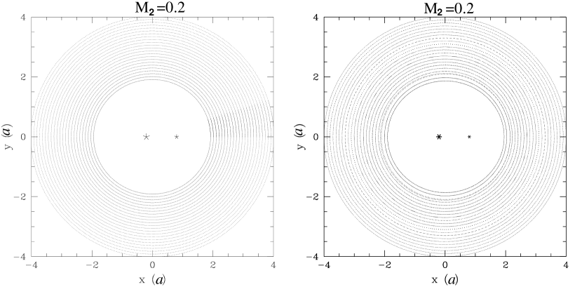
Figure 2: Circumbinary discs comparison between orbits with the approximation presented in this work and numerical results described in subsection 4.1 for the case $M_{2}=0.2$. Left panel shows the analytical approximation provided in this work. Right panel shows the numerical approximation. The axes are in units of the distance between the stars, $a$. The distance of the primary and secondary star with respect to the center of mass of the system is indicated by the black asterisks

The discs present a slight deformation of the orbits depending on the radius: the outermost orbits are farer from being circles. The orbits are, a very good approximation, ellipses with an eccentricity depending on the radius to the central star, in the cincumstellar discs, and to the center of mass in the circumbinary discs case. Thus, we have calculated the m=2 Fourier mode for all the orbits given by

$$A_{k}=\frac{1}{N}\sum_{i=0}^{N}s(\phi_{i})cos(k\phi_{i}),\,$$

$$B_{k}=\frac{1}{N}\sum_{i=0}^{N}s(\phi_{i})sin(k\phi_{i})\,,$$ (53)

where the index $i$ refers to the number of evenly distributed (by interpolation) in angle points in a given loop, and $N$ is the total number of points in the loop, $s(\phi_{i})$ is the distance to the point $i$ from the center of mass of the binary. In this manner, the average inner radius of a circumbinary disk is given in units of the semimajor axis $a$ by the coefficient $A_{K}$ with $k=0$. The ellipticity ($ell$) by $\sqrt{A_{k}^{2}+B_{k}^{2}}$ with $k=2$ in the same units and transformed first to the ratio $b_{i}/a_{i}$, where $a_{i},b_{i}$ are the semimajor and semiminor axis of the orbit $i$, and finally transformed to eccentricity ($ecc$) by,

$$ecc=\sqrt{1-ell^{2}}$$ (54)

which represents a more sensitive geometrical characteristic of the orbits than ellipticity. We have not considered in this comparison higher Fourier modes since they are negligible compared to the m=2 mode.

In the Figure 3 we show the eccentricity vs the average radius for a) the orbits produced by the analytical approximation provided in this work (continuous lines in the 9 frames), b) the full numerical solution (open triangles), and for reference c) the keplerian ($ecc=0$) solution (dashed lines). In this figure we show three different masses $M_{2}=0.01,0.2,0.4$, at left, middle and right panels respectively (as indicated on the upper frames labels). The upper frames are referred to the circumprimary discs, the middle to the circumsecondary discs, and the lower are the circumbinary discs. The system of reference for each case is on the respective star for the circumstellar discs and in the center of mass for the circumbinary discs.

Figure 3: Comparison between the orbital eccentricity vs radius produced by the analytical approximation provided in this work (continuous lines), the full numerical solution (open triangles), and for reference the keplerian ($ecc=0$) solution (dashed straight lines). Three examples of different masses, $M_{2}=0.01,0.2,0.4$, are indicated by the upper labels at left, middle and right panels respectively. The upper frames are referred to the circumprimary discs, the middle to the circumsecondary discs, and the lower are the circumbinary discs

4.3 Rotation Curves

We also show here, for a quantitative comparison involving positions and velocities, the rotation curves for binary systems with $M_{2}=0.01,0.2,0.4$.

We have constructed the rotation curves by direct differentiation of equations 6 and 7 (or more precisely of equations 51 and 52), to obtain the total velocity ($v_{c}$) at two different regions of the discs. For the primary discs we compared the rotation curves obtained along the x axis, on the left part of the discs (where the radial velocities are negative and prograde with the rotation of the binary). For the secondary we chose to compare the rotation curves along the x axis but on the right part of the disc (where the radial velocities are positive and prograde with the rotation of the binary). Once the velocities are calculated, we transformed the results to the inertial frame (in the circumstellar discs) by simply adding (or subtracting depending on the given disc) the velocity of the correspondent star, and adding or subtracting also a factor $\Omega r$, where $\Omega$ is the angular velocity of the star and $r$ is the radius of a given point in he rotation curve. The last because of the chosen reference system where this work solves the equations, which anchorages the discs to rotate with the system.

In the Figure 4 and 5 we show the outer (top panels) and inner (bottom panels) regions of the primary and secondary rotation curve discs, respectively. By “outer” or “inner” regions we mean, in a reference system located in the primary (or in the secondary) star, measuring and angle from the line that joins the stars, the inner region corresponds to angle zero from this line, and the outer regions correspond to and angle of $180^{o}$. For both figures we plot the three different cases, $M_{2}=0.01,0.2,0.4$. Three different types of lines indicate, a)the keplerian rotation curve on the top (filled circles); b) the analytical approximation provided in this work (continuous line); c) the numerical solution (open circles). The velocity and radius are given in code units (in such a way that $G=1$, $M_{1}+M_{2}=1$, $a=1$ and $\Omega=1$).

Figure 4: Comparison between the keplerian rotation curve (filled circles), the analytical approximation provided in this work (continuous line), and the numerical solution (open circles), for the outer region (top frame), and inner region (bottom frame) of the primary disc, in the different cases $M_{2}=0.01,0.2,0.4$.

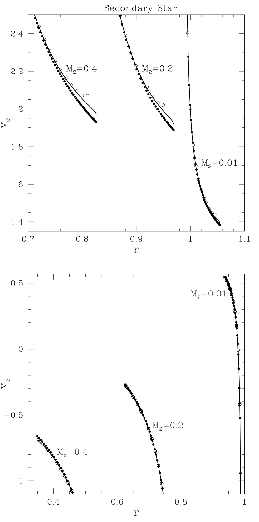
Figure 5: Same as Figure 4 but for the secondary star

The rotation curves are in approximately 70$\%$ of the total radius of the correspondent disc, keplerian curves. For the last 30$\%$ the keplerian discs velocity are systematically over the numerical result that solves with high precision the restricted three body problem. The analytical solution we provide here is very close to the numerical solution as expected.

In the Figure 6 we show the rotation curves as in Figures 4 and 5, but for the circumbinary disc. Although in this case both approximations (the one given in this work, and the numerical one) are very close to a keplerian rotation curve, it is not exactly keplerian. The velocities in the analytical approximation are sistematically under the keplerian curve and they are practically the same as the ones provided by the numerical solution, until the end (the beginning of the gap) where the numerical solution goes slightly over the analytical solution. We present only one case of mass ratio because other mass ratio would give very similar results.

Figure 6: Comparison between the keplerian rotation curve (filled circles), the analytical approximation provided in this work (continuous line), and the numerical solution (open circles), for the left region (top panel), and right region (bottom panel) of the circumbinary disc, for $M_{2}=0.2$.

In the case of the full (numerical) solution, it is worth to notice we obtain in some cases discotinuities on the rotation curves and orbits mainly due to resonances. This is the case, for instance, in the Figure 6, where we appreciate a discontinuity very close to the resonance 3:1 ($r\sim-2.1a$ in the figure). The discontinuity is also noticeable in the Fig. 2 at the same radius. Due to the perturative fit performed in this work, finding this kind of discontinuities due to resonances, that result in general very narrow in radius but where the physics is highly non-linear is out of the reach of our approach.

5 CONCLUSIONS

We have constructed an analytical set of equations based on perturbative analysis that result simple and precise to approximate the solution for the circular restricted three body problem. We choose some terms in the expanded equations of motion, which are relevant to the solution of the problem. The original equations are approximated with a set of equations that, in many cases, have an analytical solution. We show the goodness of our analytical approximation by direct comparison of geometry and rotation curves with the full numerical solution.

The set of equations we prsent can provide any periodic orbit for a binary system, either circumstellar or circumbinary, and not only the outer edge radius of circumstellar discs or the inner edge radius (gap) of the circumbinary disc, without the need to solve the problem numerically.

The relations provided are simple and straightforward in such a way that our approximation can be used for any application where initial conditions of periodic orbits or complete periodic orbits are needed, or for direct study of the three body restricted circular problem. For instance, in order to introduce on a hydrodynamical or particle code, our initial conditions would result in much more stable discs than with keplerian initial conditions, or than by constructing the discs directly from hydrodynamical simulations of accretion to binaries that will require long times to obtain stable discs. Since our approximation is completely analytical it will have the obvious additional advantage of being computationally, extremely cheap, and easier to implement than the numerical solution.

The periodic orbits respond uniquely to the binary potential and do not consider other physical factors such as gas pressure, or viscosity that work to build the fine details of discs structure. They are however, the backbone of any potential and their shape and behavior give the general discs phase space structure. In this manner, apart of all the possible hydrodynamical or particle discs applications, we can directly use them to study from the general discs geometry to rotation curves, or rarification and compression zones by orbital crowding, etc.

References

- Bate (1997) Bate, M. R., 1997, MNRAS, 285, 16
- Bate & Bonnell (1997) Bate, M. R. & Bonnell, I. A. 1997, MNRAS, 285, 33
- Bonnell & Bastien (1992) Bonnell, I. & Bastien, P. 1992, IAU Colloquium 135, 32, 206
- Butler et al. (1997) Butler, R. P., Marcy, G. W., Williams, E., Hauser, H. & Shirts, P. 1997, ApJ, 474, 115
- Cochran et al. (1997) Cochran, W. D., Hatzes, A. P., Butler, R. P. & Marcy, G. W. 1997, ApJ, 483, 457
- Duquennoy & Mayor (1991) Duquennoy, A. & Mayor, M. 1991, A&A, 248, 485
- Eggleton (1983) Eggleton, P. P. 1983, ApJ, 268, 368
- Fischer & Marcy (1992) Fischer, D. A. & Marcy, G. W. 1992, ApJ, 396, 178
- Holman & Wiegert (1999) Holman, M. J. & Wiegert P. A. 1999, AJ, 117, 621
- Lubow & Shu (1975) Lubow, S. H. & Shu, F. H. 1975, ApJ, 198, 383
- Murray & Dermott (1999) Murray, C.D. & Dermott, S.F. 1999, Solar System Dynamics, Cambridge University Press, p. 229.
- Mathieu (1994) Mathieu, R. D. 1994, ARA&A, 32, 465
- Mathieu (2000) Mathieu, R. D., Ghez, A. M., Jensen, E. L. N. & Simon, M. 2000, in Protostar and Planets IV, ed. V. Mannings, A. P. Boss & S. S. Russell (Tucson: Univ. Arizona Press) 731
- Message (1959) Message, P. J. 1959, AJ, 64, 226
- Moulton (1963) Moulton, F.R., Periodic Orbits, Washington: Carnegie institution of Washington, 1963 c1920.
- Papaloizou & Pringle (1977) Papaloizou, J. & Pringle, J. E. 1977, 181, 441
- Paczyński (1977) Paczyński, B. 1977, ApJ, 216, 822
- Pichardo, Sparke & Aguilar (2005) Pichardo, B., Sparke, L. S. & Aguilar, L. A. 2005, MNRAS, 359, 521
- Rodríguez et al. (1998) Rodríguez, L. F., D’alessio, P., Wilner, D. J., Jo, P. T. P., Torrelles, J. M., Curiel, S., Gómez, Y., Lizano, S., Pedlars, A., Cantó, J. & Raga, A. C. 1998, Nature, 395, 355
- Rudak & Paczyński (1981) Rudak, B., Paczyński, B. 1981, Acta Astron, 31, 13
- Wiegert, Holman (1997) Wiegert, P. A., Holman, M. J. 1997, AJ, 113, 1445