P- and D-wave spin-orbit splittings in heavy-light mesons

Abstract:

This is a summary of a detailed study of heavy-light meson excited state energies. Our lattice measurements include both radial and orbital excitations. Particular attention is paid to the spin-orbit splittings, to see which one of the states (for a given angular momentum L) has the lower energy. In nature the closest equivalent of this heavy-light system is the $B_{s}$ meson, which allows us to compare our lattice calculations to experimental results (where available) or give a prediction where the excited states, particularly P-wave states, should lie.

1 Introduction

The excited state spectrum of $D_{s}$ and $B_{s}$ mesons has attracted a lot of interest lately. For example, last year (2006) CDF and DØ collaborations reported measurements of two $B_{s}$ meson P-wave states [1], and BaBar and Belle measured excited $D_{s}$ meson states [2, 3]. Lattice QCD has now an excellent opportunity to offer some knowledge in the matter from the theory side. We have done an in-depth study of a heavy-light meson excited state energy spectrum on a lattice. This proceedings paper offers a summary of our results. Full details of the study can be found in [4].

We have measured the energies of both angular and first radial excitations of heavy-light mesons. Since the heavy quark is static, its spin does not play a role in the measurements. We may thus label the states as $\mathrm{L}_{\pm}=\mathrm{L}\pm\frac{1}{2}$, where L is the orbital angular momentum and $\pm\frac{1}{2}$ is the spin of the light quark.

Our main measurements are done on a $16^{3}\!\times\!32$ lattice with 160 configurations. The two degenerate quark flavours have a mass that is close to the strange quark mass (about 1.1$m_{s}$). The lattice configurations were generated by the UKQCD Collaboration using lattice action parameters $\beta=5.2$, $c_{\textrm{SW}}=2.0171$ and $\kappa=0.1350$. The lattice spacing is $\approx 0.11$ fm. More details of the lattice configurations used in this study can be found in Refs. [5, 6]. Because the light quarks are heavier than true u and d quarks, the pion mass is $m_{\pi}=0.73(2)$ GeV. Two different levels of fuzzing (2 and 8 iterations of conventional fuzzing) are used in the spatial directions to permit a cleaner extraction of the excited states.

We also introduce two types of smearing in the time direction. First we try APE type smearing, where the original links in the time direction are replaced by a sum over the six staples that extend one lattice spacing in the spatial directions (“sum6” for short). To smear the static quark even more we then use hypercubic blocking (“hyp” for short), but again only in the time direction. The label “static” is used to denote the heavy quark that is not smeared in the time direction.

2 Energy spectrum

To obtain the energy spectrum we measure the 2-point correlation function

$$C_{2}(T)=\langle P_{t}\Gamma G_{q}(\mathbf{x},t+T,t)P_{t+T}\Gamma^{{\dagger}}U^{Q}(\mathbf{x},t,t+T)\rangle\ ,$$ (1)

where $U^{Q}(\mathbf{x},t,t+T)$ is the heavy (infinite mass)-quark propagator and $G_{q}(\mathbf{x},t+T,t)$ the light anti-quark propagator. $P_{t}$ is a linear combination of products of gauge links at time $t$ along paths $P$ and $\Gamma$ defines the spin structure of the operator. The $\langle...\rangle$ denotes the average over the whole lattice. A detailed discussion of lattice operators for orbitally excited mesons can be found in [7]. In this study, the same operators are used as in [8]. The energies ($m_{i}$) and amplitudes ($a_{i}$) are extracted by fitting the $C_{2}$ with a sum of exponentials,

$$[C_{2}(T)]_{f_{1},f_{2}}\approx\sum_{i=1}^{N_{\textrm{max}}}a_{i,f_{1}}\mathrm{e}^{-m_{i}T}a_{i,f_{2}},\;\textrm{where $N_{\textrm{max}}=2\textrm{ -- }4$, $T\leq 14$}.$$ (2)

In most of the cases 3 exponentials are used to try to ensure the first radially excited states are not polluted by higher states. Also 2 and 4 exponential fits were used to cross-check the results wherever possible. Indices $f_{1}$ and $f_{2}$ denote the amount of fuzzing.

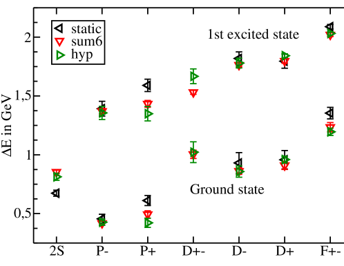
Figure 1: Energy spectrum of the heavy-light meson. Here L$+$($-$) means that the light quark spin couples to angular momentum L giving the total $j=\textrm{L}\pm 1/2$. The 2S is the first radially excited L$=0$ state. The D$+-$ is a mixture of the D$-$ and D$+$ states, and likewise for the F$+-$. Energies are given with respect to the S-wave ground state (1S). Here $a=0.110(6)$ fm is used to convert the energies to physical units. The error bars shown here contain statistical errors only.

nL$\pm$	static	sum6	hyp	nL$\pm$	static	sum6	hyp
1S	3.60(4)	2.805(14)	2.51(2)	2S	5.40(5)	5.08(4)	4.67(8)
1P$-$	4.82(10)	3.92(4)	3.64(7)	2P$-$	7.31(16)	6.45(6)	6.11(15)
1P$+$	5.23(10)	4.12(8)	3.63(10)	2P$+$	7.83(13)	6.62(8)	6.09(16)
1D$\pm$	-	5.48(10)	5.22(17)	2D$\pm$	-	6.88(4)	6.94(14)
1D$-$	6.08(14)	5.10(7)	4.79(12)	2D$-$	8.44(10)	7.50(4)	7.24(11)
1D$+$	6.15(20)	5.22(9)	5.06(7)	2D$+$	8.38(15)	7.59(5)	7.41(4)
1F$\pm$	7.21(12)	6.09(10)	5.69(8)	2F$\pm$	9.16(3)	8.18(4)	7.88(2)

Table 1: Heavy-light meson energies on the lattice in units of $r_{0}$. Here $r_{0}/a=4.754(40)(+2-90)$ (Ref. [5]), which means $r_{0}\approx 0.52$ fm. The n denotes the radial excitation and n$-1$ gives the number of nodes in the wavefunction of the state.

The extracted energy spectrum is shown in Fig. 1. In most cases, using different smearing for the heavy quark does not seem to change the energies significantly — the exceptions being the P$+$ (and excited D$+-$) state. The energy of the D$+-$ state had been expected to be near the spin average of the D$-$ and D$+$ energies, but it turns out to be a poor estimate of this average. Therefore, it is not clear to what extent the F$+-$ energy is near the spin average of the two F-wave states, as was originally hoped.

2.1 Interpolation to the b-quark mass

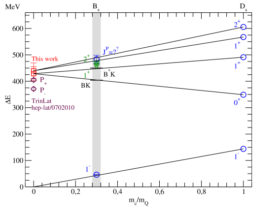
Figure 2: Interpolation to the b-quark mass. The ratio $m_{c}/m_{b}$ is taken to be $0.30(2)$ (from [9]; shown by the vertical band). The $D_{s}$ meson experimental results are from [9] (blue circles), and the $B_{s}$ meson experimental results are from [9] (blue circles) and [1] (green triangles). TrinLat group’s $m_{c}/m_{Q}=0$ results (maroon diamonds) are from [10]. Our results (using “hyp” configurations) are marked with red squares. The agreement with the measured $B_{s}$ meson P-wave states is very good as seen in Table 2. If the “sum6” lattice results were used instead of the “hyp” results, the predicted energies at $m_{c}/m_{b}$ would be too high compared to experiments.

JP	hyp	sum6	experiments
$0^{+}$	$405\pm 20$ MeV	$399\pm 12$ MeV	-
$1^{+}$	$447\pm 20$ MeV	$441\pm 12$ MeV	-
$1^{+}$	$477\pm 22$ MeV	$517\pm 22$ MeV	$460\pm 3$ MeV
$2^{+}$	$489\pm 22$ MeV	$528\pm 22$ MeV	$470\pm 3$ MeV

Table 2: Our predictions for $B_{s}$ meson mass differences, M(B${}^{\ast}_{s}$)-M(B_s), for the P-wave states. The uncertainty in the ratio $m_{c}/m_{b}$ was not taken into account in the error estimates. The experimental results are from [1, 9]. Here the “hyp” lattice P$+$ energy is taken to be E(P$-$) + spin-orbit splitting = 440(30) MeV instead of the direct lattice measurement E($P+$) = 423(39) MeV. The latter would lead to predictions E($1^{+}$) = 466(28) MeV and E($2^{+}$) = 477(28) MeV for the $B_{s}$ meson.

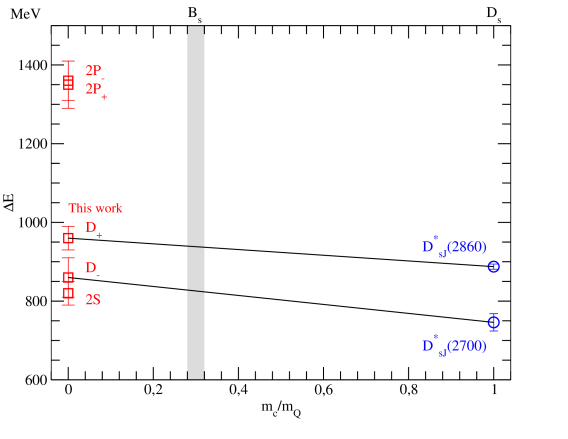
Figure 3: Interpolation to the b-quark mass: higher excited states. The lines illustrate what the interpolation would look like, if the $D_{s}$ meson states were D-wave states. The experimental results are from [2, 3]. Interpolating to $m_{c}/m_{b}$ predicts D-wave $J^{P}=3^{-}$, $J^{P}=1^{-}$ at 938(23) and 826(42) MeV respectively.

One way to obtain predictions of the $B_{s}$ meson excited state energies is to interpolate in $1/m_{Q}$, where $m_{Q}$ is the heavy quark mass, between the static heavy quark lattice calculations and $D_{s}$ meson experimental results, i.e. interpolate between the static quark ($m_{Q}=\infty$) and the charm quark ($m_{Q}=m_{c}$). Here we, of course, have to assume that the measured $D_{s}$ meson states are simple quark–anti-quark states. This is not necessarily true: for example the mass of the $D_{s0}^{\ast}(2317)$ is much lower than what is predicted by conventional potential models, and it has thus been proposed that it could be either a four quark state, a $DK$ molecule or a $D\pi$ atom. However, the inclusion of chiral radiative corrections could change the potential model predictions considerably [11]. Here we assume simple quark–anti-quark states and do a linear interpolation (see Fig. 2). The two lowest P-wave states seem to lie only a couple of MeV below the $BK$ and $B^{\ast}K$ thresholds respectively. Our predictions are given in Table 2.

As for other excited states, BaBar and Belle observed two new states, $D_{sJ}^{\ast}(2860)$ and $D_{sJ}^{\ast}(2700)$, in 2006 [2, 3]. The $J^{P}$ quantum numbers of the $D_{sJ}^{\ast}(2860)$ can be $0^{+}$, $1^{-}$, $2^{+}$, etc., so it could be a radial excitation of the $D_{s0}^{\ast}(2317)$ or a $J^{P}=3^{-}$ D-wave state. The first interpretation is rather popular, but our lattice results favour the D-wave $J^{P}=3^{-}$ assignment in agreement with Colangelo, De Fazio and Nicotri [12]. Interpolation then predicts a D-wave $J^{P}=3^{-}$ $B_{s}$ state at 938(23) MeV. The alternative interpretation as a 2P state, when compared with our lattice result, would lead to an unreasonably large $1/m_{Q}$ dependence. In addition, the $D_{sJ}^{\ast}(2700)$ could be a radially excited S-wave state or a D-wave $J^{P}=1^{-}$ state. If the latter identification is assumed, then a D-wave $J^{P}=1^{-}$ $B_{s}$ state at 826(42) MeV is expected (see Fig. 3).

2.2 Spin-orbit splitting

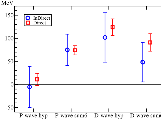
Figure 4: The spin-orbit splittings of P-wave and D-wave states. The P-wave spin-orbit splitting is small (consistent with zero), whereas the D-wave spin-orbit splitting is much larger and positive.

E(nL$+$) $-$ nE(L$-$)	Indirect	Direct
E(1P$+$) $-$ E(1P$-$)	$-5\pm 45$ MeV	$11\pm 13$ MeV
E(1D$+$) $-$ E(1D$-$)	$102\pm 54$ MeV	$124\pm 18$ MeV
E(2P$+$) $-$ E(2P$-$)	$-10\pm 83$ MeV	-
E(2D$+$) $-$ E(2D$-$)	$70\pm 60$ MeV	-

Table 3: P-wave and D-wave spin-orbit splittings using “hyp” configurations.

We pay particular attention to the spin-orbit splitting (SOS) of the P-wave states, i.e. the energy difference of the 1P$+$ and 1P$-$ states. We extract the SOS in two different ways:

1. Indirectly by simply calculating the difference using the energies given by Eq. 2, when the P$+$ and P$-$ data are fitted separately.

2. Combining the P$+$ and P$-$ data and fitting the ratio $\textrm{C}_{2}(\textrm{P}+)/\textrm{C}_{2}(\textrm{P}-)$, which enables us to go directly for the spin-orbit splitting, $m_{\textrm{1P$+$}}-m_{\textrm{1P$-$}}$.

The D-wave spin-orbit splitting is also extracted in a similar manner. The results of the fits are given in Table 3 and in Fig. 4. The two smearings, “sum6” and “hyp”, give different spin-orbit splittings for the P-wave: 74(10) MeV and 11(13) MeV, respectively. This is unexpected, and is studied in detail in [4]. A similar difference is not seen in the D-wave, where direct analysis gives 124(18) MeV (“hyp”) and 91(19) MeV (“sum6”).

3 Conclusions

• With the “hyp” lattice, our predictions for the $1^{+}$ and $2^{+}$ P-wave state masses agree very well with the experimental results. We also predict that the masses of the two lower P-wave states ($0^{+}$ and $1^{+}$) should lie only a few of MeV below the $BK$ and $B^{\ast}K$ thresholds respectively.

• Also with the “hyp” lattice, the P-wave spin-orbit splitting is small (essentially zero), but the D-wave spin-orbit splitting is clearly non-zero and positive. In contrast, another lattice group finds the D-wave spin-orbit splitting to be slightly negative (see [10]), i.e. they seem to observe the famous inversion [13]. On the other hand, in [11] Woo lee and Lee suggest that the absence of spin-orbit inversions can be explained by chiral radiative corrections in the potential model.

References

- [1] CDF and DØ collaborations, R. K. Mommsen, hep-ex/0612003
- [2] BABAR Collaboration, B. Aubert, Phys. Rev. Lett. 97, 222001 (2006)
- [3] Belle Collaboration, K. Abe et al., arXiv:hep-ex/0608031
- [4] UKQCD Collaboration, J. Koponen, arXiv:0708.2807 [hep-lat]
- [5] C. R. Allton et al. (UKQCD Collaboration), Phys. Rev. D 65, 054502 (2002)
- [6] UKQCD Collaboration, A. M. Green, J. Koponen, C. Michael, C. McNeile and G. Thompson, Phys. Rev. D 69, 094505 (2004), and UKQCD Collaboration, J. Koponen, hep-lat/0411015
- [7] UKQCD Collaboration, P. Lacock, C. Michael, P. Boyle and P. Rowland, Phys. Rev. D 54, 6997 (1996)
- [8] UKQCD Collaboration, C. Michael and J. Peisa, Phys. Rev. D 58, 034506 (1998)
- [9] W.-M. Yao et al., J. Phys. G 33, 1 (2006)
- [10] J. Foley, A. Ó Cais, M. Peardon and S. Ryan, PoS LAT2006 (2006) 196 and hep-lat/0702010
- [11] I. Woo Lee and T. Lee, Phys. Rev. D 76, 014017 (2007)
- [12] P. Colangelo, F. De Fazio and S. Nicotri, Phys. Lett. B 642, 48 (2006)
- [13] H. J. Schnitzer, Phys. Rev. D 18, 3482 (1978) and Phys. Lett. B 226, 171 (1989)