Q-adic Transform Revisited

Abstract

We present an algorithm to perform a simultaneous modular reduction of several residues. This enables to compress polynomials into integers and perform several modular operations with machine integer arithmetic. The idea is to convert the $X$-adic representation of modular polynomials, with $X$ an indeterminate, to a $q$-adic representation where $q$ is an integer larger than the field characteristic. With some control on the different involved sizes it is then possible to perform some of the $q$-adic arithmetic directly with machine integers or floating points. Depending also on the number of performed numerical operations one can then convert back to the $q$-adic or $X$-adic representation and eventually mod out high residues. In this note we present a new version of both conversions: more tabulations and a way to reduce the number of divisions involved in the process are presented. The polynomial multiplication is then applied to arithmetic and linear algebra in small finite field extensions.

Keywords:

Kronecker substitution ; Finite field ; Modular Polynomial Multiplication ; REDQ (simultaneous modular reduction) ; Small extension field ; DQT (Discrete Q-adic Transform) ; FQT (Fast Q-adic Transform).

1 Introduction

The FFLAS/FFPACK project has demonstrated the usefulness of wrapping cache-aware routines for efficient small finite field linear algebra [4, 5].

A conversion between a modular representation of prime fields and e.g. floating points used exactly is natural. It uses the homomorphism to the integers. Now for extension fields (isomorphic to polynomials over a prime field) such a conversion is not direct. In [4] we proposed transforming the polynomials into a $q$-adic representation where $q$ is an integer larger than the field characteristic. We call this transformation DQT for Discrete Q-adic Transform, it is a form of Kronecker substitution [7, §8.4]. With some care, in particular on the size of $q$, it is possible to map the operations in the extension field into the floating point arithmetic realization of this $q$-adic representation and convert back using an inverse DQT.

In this note we propose some implementation improvements: we propose to use a tabulated discrete logarithm for the DQT and we give a trick to reduce the number of machine divisions involved in the inverse. This then gives rise to an improved DQT which we thus call FQT (Fast Q-adic Transform). This FQT uses a simultaneous reduction of several residues, called REDQ, and some table lookup.

Therefore we recall in section 2 the previous conversion algorithm and discuss in section 3 about a floating point implementation of modular reduction. This implementation will be used throughout the paper to get fast reductions. We then present our new simultaneous reduction in section 4 and show in section 5 how a time-memory trade-off can make this reduction very fast. This fast reduction is then applied to modular polynomial multiplication with small prime fields in section 6. It is also applied to small extension field arithmetic and fast matrix multiplication over those fields in section 7.

2 Q-adic representation of
polynomials

We follow here the presentation of [4] of the idea of [12]: polynomial arithmetic is performed a $q-$adic way, with $q$ a sufficiently big prime or power of a single prime.

Suppose that $a=\sum_{i=0}^{k-1}\alpha_{i}X^{i}$ and $b=\sum_{i=0}^{k-1}\beta_{i}X^{i}$ are two polynomials in $\leavevmode\kern 1.00006pt\raise 0.0pt\hbox{$\mathbb{Z}$}\kern-1.00006pt/\kern-1.49994pt\lower 1.29167pt\hbox{p\mbox{$\mathbb{Z}$}}[X]$. One can perform the polynomial multiplication $ab$ via $q-$adic numbers. Indeed, by setting $\tilde{a}=\sum_{i=0}^{k-1}\alpha_{i}q^{i}$ and $\tilde{b}=\sum_{i=0}^{k-1}\beta_{i}q^{i}$, the product is computed in the following manner (we suppose that $\alpha_{i}=\beta_{i}=0$ for $i>k-1$):

$$\widetilde{ab}=\sum_{j=0}^{2k-2}\left(\sum_{i=0}^{j}\alpha_{i}\beta_{j-i}\right)q^{j}$$ (1)

Now if $q$ is large enough, the coefficient of $q^{i}$ will not exceed $q-1$. In this case, it is possible to evaluate $a$ and $b$ as machine numbers (e.g. floating point or machine integers), compute the product of these evaluations, and convert back to polynomials by radix computations (see e.g. [7, Algorithm 9.14]). There just remains then to perform modulo $p$ reductions on every coefficient as shown on example 1.

Example 1.

For instance, to multiply $a=X+1$ by $b=X+2$ in $\leavevmode\kern 1.00006pt\raise 0.0pt\hbox{$\mathbb{Z}$}\kern-1.00006pt/\kern-1.49994pt\lower 1.29167pt\hbox{3\mbox{$\mathbb{Z}$}}[X]$ one can use the substitution $X=100$: compute $101\times 102=10302$, use radix conversion to write $10302=q^{2}+3q+2$ and reduce modulo $3$ to get $a\times b=X^{2}+2$.

We call DQT the evaluation of polynomials modulo $p$ at $q$ and DQT inverse the radix conversion of a $q$-adic development followed by a modular reduction, as shown in algorithm 1.

Algorithm 1 Polynomial multiplication by DQT

0:  Two polynomials $v_{1}$ and $v_{2}$ in $\leavevmode\kern 1.00006pt\raise 0.0pt\hbox{$\mathbb{Z}$}\kern-1.00006pt/\kern-1.49994pt\lower 1.29167pt\hbox{p\mbox{$\mathbb{Z}$}}[X]$ of degree less than $k$.

0:  a sufficiently large integer $q$.

0:  $R\in\leavevmode\kern 1.00006pt\raise 0.0pt\hbox{$\mathbb{Z}$}\kern-1.00006pt/\kern-1.49994pt\lower 1.29167pt\hbox{p\mbox{$\mathbb{Z}$}}[X]$, with $R=v_{1}.v_{2}$.
Polynomial to $q-$adic conversion

1:  Set $\widetilde{v_{1}}$ and $\widetilde{v_{2}}$ to the floating point vectors of the evaluations at $q$ of the elements of $v_{1}$ and $v_{2}$. {Using e.g. Horner’s formula}
One computation

2:  Compute $\tilde{r}=\widetilde{v_{1}}\widetilde{v_{2}}$
Building the solution

3:  $\tilde{r}=\sum_{i=0}^{2k-2}\widetilde{\mu_{i}}q^{i}$. {Using radix conversion, see e.g. [7, Algorithm 9.14]}

4:  For each $i$, set $\mu_{i}=\widetilde{\mu_{i}}\mod p$

5:  set $R=\sum_{i=0}^{2k-2}\mu_{i}X^{i}$

Depending on the size of $q$, the results can still remain exact and we obtain the following bounds generalizing that of [7, §8.4]:

Theorem 1.

[4] Let $m$ be the number of available mantissa bits within the machine numbers and $n_{q}$ be the number of polynomial products $v_{1}.v_{2}$ of degree $k$ accumulated before the re-conversion. If

$$q>n_{q}k(p-1)^{2}\text{~{}and~{}}(2k-1)\log_{2}(q)<m,$$ (2)

then Algorithm 1 is correct.

Note that the integer $q$ can be chosen to be a power of 2. Then the Horner like evaluation (line 1 of algorithm 1) of the polynomials at $q$ is just a left shift. One can then compute this shift with exponent manipulations in floating point arithmetic and use native shift operator (e.g. the $<<$ operator in C) as soon as values are within the $32$ (or $64$ when available) bit range.

It is shown on [4, Figures 5 & 6] that this wrapping is already a pretty good way to obtain high speed linear algebra over some small extension fields. Indeed we were able to reach high peak performance, quite close to those obtained with prime fields, namely 420 Millions of finite operations per second (Mop/s) on a Pentium III, 735 MHz, and more than 500 Mop/s on a 64-bit DEC alpha 500 MHz. This was roughly 20 percent below the pure floating point performance and 15 percent below the prime field implementation.

3 Euclidean division by floating point routines

In the implementations of the proposed subsequent algorithms, we will make extensive use of Euclidean division in exact arithmetic. Unfortunately exact division is usually quite slow on modern computers. This division can thus be performed by floating point operations. Suppose we want to compute $r/p$ where $r$ and $p$ and integers. Then their difference is representable by a floating point and, therefore, if $r/p$ is computed by a floating point division with a rounding to nearest mode, [9, Theorem 1] assures that flooring the result gives the expected value. Now if a multiplication by a precomputed inverse of $p$ is used (as is done e.g. in NTL [13]), proving the correctness for all $r$ is more difficult, see [10] for more details. We therefore propose the following simple lemma which enables the use of the rounding upward mode to the cost of loosing only one bit of precision:

Lemma 1.

For two positive integers $p$ and $r$ and $\epsilon>0$, we have

$$\left\lfloor\frac{r}{p}\right\rfloor=\left\lfloor\left(r\left(\frac{1}{p}(1+\epsilon)\right)\right)(1+\epsilon)\right\rfloor~{}~{}\text{as long as}~{}~{}r<\frac{1}{2\epsilon+\epsilon^{2}}.$$

Proof.

Consider $up\leq r<up+i$ with $u,i$ positive integers and $i<p$. Then $\left\lfloor\frac{r}{p}\right\rfloor=u$ and $\frac{r}{p}(1+\epsilon)(1+\epsilon)=u+\frac{i}{p}+\frac{r}{p}(2\epsilon+\epsilon^{2})$. The latter is maximal at $i=p-1$. This proves that flooring is correct as long as $\frac{r}{p}(2\epsilon+\epsilon^{2})<\frac{1}{p}$. ∎

This proves that when rounding towards $+\infty$ it is possible to perform the division by a multiplication by the precomputed inverse of the prime number as long as $r$ is not too large. Since our entries will be integers but stored in floating point format this is a potential significant speed-up.

4 REDQ: modular reduction in the DQT domain

The first improvement we propose to the DQT is to replace the costly modular reduction of the polynomial coefficients by a single division by $p$ (or, better, by a multiplication by its inverse) followed by several shifts. In order to prove the correctness of this algorithm, we first need the following lemma:

Lemma 2.

For $r\in\mathbb{N}$ and $a$, $b\in\mathbb{N}^{*}$,

$$\left\lfloor\frac{\left\lfloor\frac{r}{b}\right\rfloor}{a}\right\rfloor=\left\lfloor\frac{r}{ab}\right\rfloor=\left\lfloor\frac{\left\lfloor\frac{r}{a}\right\rfloor}{b}\right\rfloor$$

Proof.

We proceed by splitting the possible values of $r$ into intervals $kab\leq r<(k+1)ab$, where $k=\left\lfloor\frac{r}{ab}\right\rfloor$. Then $kb\leq\frac{r}{a}<(k+1)b$ and since $kb$ is an integer we also have that $kb\leq\left\lfloor\frac{r}{a}\right\rfloor<(k+1)b$. Thus $k\leq\frac{\left\lfloor\frac{r}{a}\right\rfloor}{b}<k+1$ and $\left\lfloor\frac{\left\lfloor\frac{r}{a}\right\rfloor}{b}\right\rfloor=k$. Obviously the same is true for the left hand side which proves the lemma. ∎

This idea is used in algorithm 2 to perform several remainderings with a single machine division (note that when $q$ is a power of $2$, and when elements are represented using an integral type, division by $q^{i}$ and flooring are a single operation, a right shift).

Algorithm 2 REDQ

0:  Two integers $p$ and $q$ satisfying the conditions (2).

0:  $\tilde{r}=\sum_{i=0}^{d}\widetilde{\mu_{i}}q^{i}\in\mathbb{Z}$.

0:  $\rho\in\mathbb{Z}$, with $\rho=\sum_{i=0}^{d}\mu_{i}q^{i}$ where $\mu_{i}=\widetilde{\mu_{i}}\mod p$.

1:   $rop=\left\lfloor\frac{\tilde{r}}{p}\right\rfloor$;

2:  for $i=0$ to $d$ do

3:      $u_{i}=\left\lfloor\frac{\tilde{r}}{q^{i}}\right\rfloor-p\left\lfloor\frac{rop}{q^{i}}\right\rfloor$;

4:  end for

5:   $\mu_{d}=u_{d}$

6:  for $i=0$ to $d-1$ do

7:     $\mu_{i}=u_{i}-qu_{i+1}\mod p$;

8:  end for

9:  Return $\rho=\sum_{i=0}^{d}\mu_{i}q^{i}$;

Theorem 2.

Algorithm REDQ is correct.

Proof.

First we need to prove that $0\leq u_{i}<p$. By definition of the truncation, we have $\frac{\tilde{r}}{q^{i}}-1<\left\lfloor\frac{\tilde{r}}{q^{i}}\right\rfloor\leq\frac{\tilde{r}}{q^{i}}$ and $\frac{\tilde{r}}{pq^{i}}-1-\frac{1}{q^{i}}<\left\lfloor\frac{rop}{q^{i}}\right\rfloor\leq\frac{\tilde{r}}{pq^{i}}$. Thus $-1<u_{i}<p+\frac{p}{q^{i}}$, which is $0\leq u_{i}\leq p$ since $u_{i}$ is an integer. We now consider the possible case $u_{i}=p$ and show that it does not happen. $u_{i}=p$ means that $\left\lfloor\frac{\tilde{r}}{q^{i}}\right\rfloor=p(1+\left\lfloor\frac{rop}{q^{i}}\right\rfloor)=pg$. This means that $pgq^{i}\leq r<pgq^{i}+q^{i}$. So that in turns $gq^{i}\leq rop\leq\frac{\tilde{r}}{p}<gq^{i}+\frac{q^{i}}{p}$. Thus $g\leq\frac{rop}{q^{i}}<g+\frac{1}{p}$ so that $\left\lfloor\frac{rop}{q^{i}}\right\rfloor=g$. But then from the definition of $g$ we have that $g=g-1$ which is absurd. Therefore $0\leq u_{i}\leq p-1$.

Second we show that $u_{i}=\sum_{j=i}^{d}\mu_{j}q^{j-i}\mod p$. Line 3 of algorithm 2 defines $u_{i}=\left\lfloor\frac{\tilde{r}}{q^{i}}\right\rfloor-p\left\lfloor\frac{\left\lfloor\frac{\tilde{r}}{p}\right\rfloor}{q^{i}}\right\rfloor$ and thus lemma 2 gives that $u_{i}=\left\lfloor\frac{\tilde{r}}{q^{i}}\right\rfloor-p\left\lfloor\frac{\left\lfloor\frac{\tilde{r}}{q^{i}}\right\rfloor}{p}\right\rfloor$. The latter is $u_{i}=\left\lfloor\frac{\tilde{r}}{q^{i}}\right\rfloor\mod p$. Now, since $\tilde{r}=\sum_{j=0}^{d}\widetilde{\mu_{j}}q^{j}$, we have that $\left\lfloor\frac{\tilde{r}}{q^{i}}\right\rfloor=\sum_{j=i}^{d}\widetilde{\mu_{j}}q^{j-i}$. Therefore, as $\mu_{j}=\widetilde{\mu_{j}}\mod p$, the equality is proven. ∎

Note that the last steps are not needed when $p$ divides $q$. Indeed in this case $q\equiv 0\mod p$. The trick works then simply as shown on example 2 below:

Example 2.

Let $a=X^{2}+2X+3$ and $b=4X^{2}+5X+6$ unreduced modulo $5$. Then $\tilde{a}\times\tilde{b}=40013002800270018$, with $q=10000$, for which we need to reduce five coefficients modulo $5$. The trick is that we can recover all the residues at once. Line 1 produces $rop=\lfloor 08002600560054003.6\rfloor$. It thus contains all the quotients $0$;$0002$;$0005$;$0005$;$0003$ and one has then just to multiply by $p$ and subtract to get: $\widetilde{a\times b}=40013002800270018-2000500050003\times 5=40003000300020003$ so that $a\times b=4X^{4}+3X^{3}+3X^{2}+2X+3$.

Now we can give a full example to show the last corrections required when $p$ does not divide $q$. The first part of the algorithm, lines 1 to 3 is unchanged and is used to get small sizes for $\mu_{i}$. The second part is then just a small correction modulo $p$ to get the correct result.

Example 3.

Take the polynomial $R=1234X^{3}+5678X^{2}+9123X+4567$, the prime $p=23$ and use $q=10^{6}$. In this case, the division gives $rop=\lfloor 1234005678009123004567/23\rfloor$ $=53652420783005348024$. Then the multiplication by the prime produces $rop\times 23=1234005678009123004552$ so that $u_{0}=4567-4552=15$. We shift to get $1234005678009123$ and $53652420783005\times 23=1234005678009115$ which gives $u_{1}=9123-9115=8$. We shift and multiply twice to get $u_{2}=18$ and $u_{3}=\mu_{3}=15$ just like in example 2. Now $-q=-10^{6}\mod 23=17$ which is non zero and thus we have to compute the corrections of lines 5 to 8 of algorithm 2. This can also be formalized as a matrix vector product:

$$\mu=\left[\begin{array}[]{cccc}1&17&0&0\\ 0&1&17&0\\ 0&0&1&17\\ 0&0&0&1\end{array}\right]u\mod p$$

to get the final result, $R=15X^{3}+20X^{2}+15X+13\mod 23$.

The algorithm is efficient because one can precompute $1/p$, $1/q$, $1/q^{2}$ etc. and use multiplication to compute all of the mods. The computation of each $u_{i}$ and $\mu_{i}$ can also be pipelined or vectorized since they are independent. As is, the benefit when compared to direct remaindering by $p$ is that the corrections occur on smaller integers. Thus the remaindering by $p$ can be faster. Actually, another major acceleration can be added: the fact that the $\mu_{i}$ are much smaller than the initial $\tilde{\mu_{i}}$ makes it possible to tabulate the corrections as shown next.

5 Time-Memory trade-off in REDQ

5.1 A Matrix version of the correction

Indeed, there is a bijection between the $u_{i}$ and the $\mu_{i}$. This can be viewed on the corrections of lines 5 to 8 of algorithm 2: view these corrections as a matrix-vector multiplication by a matrix $Q_{d}$ as in example 3. Then we have that:

$$Q_{d}=\left[\begin{array}[]{ccccc}1&-q&0&\ldots&0\\ 0&\ddots&\ddots&\ddots&\vdots\\ \vdots&\ddots&\ddots&\ddots&0\\ \vdots&&\ddots&\ddots&-q\\ 0&\ldots&\ldots&0&1\end{array}\right]=\left[\begin{array}[]{ccccc}1&q&q^{2}&\ldots&q^{d}\\ 0&\ddots&\ddots&\ddots&\vdots\\ \vdots&\ddots&\ddots&\ddots&q^{2}\\ \vdots&&\ddots&\ddots&q\\ 0&\ldots&\ldots&0&1\end{array}\right]^{-1}$$

5.2 Tabulations of the matrix-vector product and Time-Memory trade-off

Thus if the multiplication by $Q_{d}$ is fully tabulated, it requires a table of size at least $p^{d+1}$. But, due to the nature of $Q_{d}$, we have the relations of figure 1.

Figure 1: Recurring relations on the $Q_{d}$ matrices.

Therefore, it is very easy to tabulate with a table of size $p^{k}$ only and perform $\left\lceil 1+\frac{d+1-k}{k-1}\right\rceil=\left\lceil\frac{d}{k-1}\right\rceil$ table accesses as shown on example 4.

Example 4.

Let us compute the corrections for a degree $6$ polynomial. One can tabulate the multiplication by $Q_{6}$, a $7\times 7$ matrix, with therefore $p^{7}$ entries each of size at least $7\log_{2}(p)$. Or one can tabulate the multiplication by $Q_{2}$, a $3\times 3$ matrix. To compute $[\mu_{0},\ldots,\mu_{6}]^{T}=Q_{6}[u_{0}\ldots,u_{6}]^{T}$ one can instead use three multiplications by $Q_{2}$ and discard the last entry for the first two multiplications as shown on the following algorithm:

Algorithm 3 $Q_{6}$ with an extra memory of size $p^{3}$

0:  $[u_{0}\ldots,u_{6}]\in\leavevmode\kern 1.00006pt\raise 0.0pt\hbox{$\mathbb{Z}$}\kern-1.00006pt/\kern-1.49994pt\lower 1.29167pt\hbox{p\mbox{$\mathbb{Z}$}}^{7}$.

0:  The table $Q_{2}$ of the associated $3\times 3$ matrix-vector multiplication over $\leavevmode\kern 1.00006pt\raise 0.0pt\hbox{$\mathbb{Z}$}\kern-1.00006pt/\kern-1.49994pt\lower 1.29167pt\hbox{p\mbox{$\mathbb{Z}$}}$.

0:  $[\mu_{0},\ldots,\mu_{6}]^{T}=Q_{6}[u_{0}\ldots,u_{6}]^{T}$.

1:  $a_{0},a_{1},a_{2}=Q_{2}[u_{0},u_{1},u_{2}]$;

2:  $b_{0},b_{1},b_{2}=Q_{2}[u_{2},u_{3},u_{4}]$;

3:  $c_{0},c_{1},c_{2}=Q_{2}[u_{4},u_{5},u_{6}]$;

4:  Return $[\mu_{0},\ldots,\mu_{6}]^{T}=[a_{0},a_{1},b_{0},b_{1},c_{0},c_{1},c_{2}]^{T}$;

When $q$ is a power of $2$, the computation of the $u_{i}$, in the first part of algorithm 2 requires $1~{}\text{div}$ & $(d+1)~{}\text{mul}$ & $2d~{}\text{shifts}$. Now, the time memory trade-off enables to compute the second part at a choice of costs given on table 1.

Extra Memory	time
$0$	$d$ (mul,add,mod)
$p^{2}$	$d$ accesses
$p^{k}$	$\left\lceil\frac{d}{k-1}\right\rceil$ accesses
$p^{d+1}$	1 access

Table 1: Time-Memory trade-off in REDQ of degree $d$ over $\leavevmode\kern 1.00006pt\raise 0.0pt\hbox{$\mathbb{Z}$}\kern-1.00006pt/\kern-1.49994pt\lower 1.29167pt\hbox{p\mbox{$\mathbb{Z}$}}$

5.3 Indexing

In practice, indexing by a t-uple of integers mod $p$ is made by evaluating at $p$, as $\sum u_{i}p^{i}$. If more memory is available, one can also directly index in the binary format using $\sum u_{i}\left(2^{\lceil\log_{2}(p)\rceil}\right)^{i}$. On the one hand all the multiplications by $p$ are replaced by binary shifts. On the other hand, this makes the table grow a little bit, from $p^{k}$ to $2^{\lceil\log_{2}(p)\rceil k}$.

6 Comparison with delayed
reduction for polynomial
multiplication

The classical alternative to algorithm 1 to perform modular polynomial multiplication is to use delayed reductions e.g. as in [1]: the idea is to accumulate products of the form $\sum_{i}a_{i}b_{k-i}$, without reductions, while the sum does not overflow. Thus, if we use for instance a centered representation modulo $p$ (integers from $\frac{1-p}{2}$ to $\frac{p-1}{2}$), it is possible to accumulate at least $n_{d}$ products as long as

$$n_{d}(p-1)^{2}<2^{m+1}$$ (3)

The modular reduction can be made by many different ways (e.g. classical division, floating point multiplication by the inverse, Montgomery reduction, etc.), we just call the best one REDC here. It is at most equivalent to 1 machine division.

Now the idea of the FQT (Fast Q-adic Transform) is to represent modular polynomials of the form $P=\sum_{i=0}^{N}a_{i}X^{i}$ by $P=\sum P_{i}\left(X^{d+1}\right)^{i}$ where the $P_{i}$ are degree $d$ polynomials stored in a single integer in the $q$-adic way.

Therefore, a product $PQ$ has the form

$$\sum\left(\sum P_{i}Q_{t-i}\right)\left(X^{d+1}\right)^{t}.$$

There, each multiplication $P_{i}Q_{t-i}$ is made by algorithm 1 on a single machine integer. The reduction is made by a tabulated REDQ and can also be delayed now as long as conditions (2) are guaranteed.

We want to compare these two strategies. We thus propose the following complexity model: we count only multiplications and additions in the field as an atomic operation and separate the machine divisions. We for instance approximate REDC by a machine division. We call REDQ_k a simultaneous reduction of $k$ residues. In our complexity model a REDQ_k thus requires $1$ division and $2k$ multiplications and additions. We also call $d-$FQT the use of a degree $d$ $q$-adic substitution. Thus a multiplication $P_{i}Q_{t-i}$ in a $d-$FQT requires the reduction of $2d+1$ coefficients, i.e. a REDQ_2d+1.

Let $P$ be a polynomial of degree $N$ with indeterminate ”X”. If we use a $d-$FQT, it will then become a polynomial of degree $D_{q}$ in the indeterminate $Y=X^{d+1}$. Thus,

$$D_{q}=\left\lceil\frac{N+1}{d+1}\right\rceil-1.$$

Table 2 gives the respective complexities of both strategies.

	Mul & Add	Reductions
Delayed	$(2N+1)^{2}$	$(2N+1)\left\lceil\frac{2N+1}{n_{d}}\right\rceil$ REDC
d-FQT	$(2D_{q}+1)^{2}$	$(2D_{q}+1)\left\lceil\frac{2D_{q}+1}{n_{q}}\right\rceil$ REDQ2d+1

Table 2: Modular polynomial multiplication complexities.

For instance, with $p=3$, $N=500$, if we choose a double floating point representation and a degree $4$ DQT, the fully tabulated FQT boils down to $10^{5}$ multiplications and additions and $4.10^{3}$ divisions. For the same parameters, the classical polynomial multiplication algorithm requires $10^{6}$ multiplications and additions and only $10^{3}$ remaindering. This is roughly $9$ times more operations as shown on figure 2.

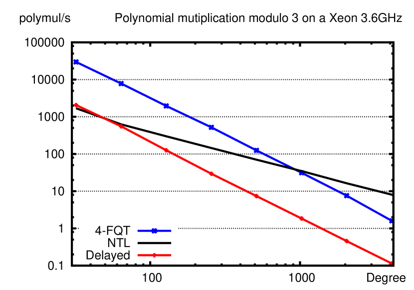
Figure 2: Polynomial multiplications modulo 3 per second on a Xeon 3.6 GHz

Even by switching to a larger mantissa, say e.g. 128 bits, so that the DQT multiplications are roughly 4 times costlier than double floating point operations, this can still be useful: take $p=1009$ and choose $d=3$, still gives around $10^{5}$ multiplications and additions over 128 bits and $4.10^{3}$ divisions. This makes $8$ times less operations. This should therefore still be faster than the delayed over $32$ bits.

On figure 2, we compare also our two implementations with that of NTL [13]. We see that the FQT is faster than NTL as long as better algorithms are not used. Indeed the change of slope in NTL’s curve reflects the use of Karatsuba’s algorithm for polynomial multiplication. One should note that NTL also proposes a very optimized modulo 2 implementation which is an order of magnitude faster than our implementation on small primes. There is therefore room for more improvements on small fields. Our strategy is anyway very useful for small degrees and small primes. Furthermore, we have not implemented the FQT as the base case of faster recursive algorithms such as Karatsuba, Toom-Cook, etc. The figure shows that these recursive algorithms together with the FQT could be the fastest.

In particular, the FQT already improves the speed of small finite field extension’s arithmetic as shown next.

7 Application to small finite
field extensions

The isomorphism between finite fields of equal sizes gives us a canonical representation: any finite field extension is viewed as the set of polynomials modulo a prime $p$ and modulo an irreducible polynomial ${\cal P}$ of degree $k$. Clearly we can thus convert any finite field element to its $q$-adic expansion ; perform the FQT between two elements and then reduce the obtained polynomial modulo ${\cal P}$. Furthermore, it is possible to use floating point routines to perform exact linear algebra as demonstrated in [6].

Our strategy here, see algorithm 4, is thus to convert vectors over $\mathtt{GF}(p^{k})$ to $q$-adic floating point, to call a fast numerical linear algebra routine (BLAS) and then to convert the floating point result back to the usual field representation. In this paper we propose to improve all the conversion steps of [4, algorithm 4.1] and thus approach the performance of the prime field wrapping also for small extension fields:

1. Replace the Horner evaluation of the polynomials, to form the $q$-adic expansion, by a single table lookup, recovering directly the floating point representation.

2. Replace the radix conversion and the costly modular reductions of each polynomial coefficient, by a single REDQ operation.

3. Replace the polynomial division by two table lookups and a single field operation.

Indeed, suppose the internal representation of the extension field is already by discrete logarithms and uses conversion tables from polynomial to index representations. See e.g. [1] for more details. Then we choose a time-memory trade-off for the REDQ operation of the same order of magnitude, that is to say $p^{k}$. The overall memory required by these new tables only doubles and the REDQ requires only $2$ accesses. Moreover, in the small extension, the polynomial multiplication must also be reduced by an irreducible polynomial, ${\cal P}$. We show next that this reduction can be precomputed in the REDQ table lookup and is therefore almost free.

Moreover, many things can be factorized if the field representation is by discrete logarithms. Indeed, the element are represented by their discrete logarithm with respect to a generator of the field, instead of by polynomials. In this case there are already some table accesses for many arithmetic operations, see e.g. [1, §2.4] for more details.

More precisely, we here propose algorithm 4 for linear algebra over extension fields: line 1 is the table look-up of floating point values associated to elements of the field ; line 2 is the numerical computation ; line 3 to 7 is the first part of the REDQ reduction ; line 8 and 9 are a time-memory trade-off with two table accesses for the corrections of REDQ, combined with a conversion from polynomials to discrete logarithm representation ; the last line 10 combines the latter two results, inside the field.

Algorithm 4 Fast Dot product over Galois fields via FQT and FQT inverse

0:  a field $\mathtt{GF}(p^{k})$ with elements represented as exponents of a generator of the field.

0:  Two vectors $v_{1}$ and $v_{2}$ of elements of $\mathtt{GF}(p^{k})$.

0:  a sufficiently large integer $q$.

0:  $R\in\mathtt{GF}(p^{k})$, with $R=v_{1}^{T}.v_{2}$.
Tabulated $q-$adic conversion
{Use conversion tables from exponent to floating point evaluation}

1:  Set $\widetilde{v_{1}}$ and $\widetilde{v_{2}}$ to the floating point vectors of the evaluations at $q$ of the elements of $v_{1}$ and $v_{2}$.
The floating point computation

2:  Compute $\tilde{r}=\widetilde{v_{1}}^{T}\widetilde{v_{2}}$;
Computing a radix decomposition

3:  $r=\lfloor\tilde{r}\rfloor$;    {$r=\tilde{r}$ but we might need a conversion to an integral type}

4:  $rop=\left\lfloor\frac{\tilde{r}}{p}\right\rfloor$;

5:  for $i=0$ to $2k-2$ do

6:     $u_{i}=\left\lfloor\frac{r}{q^{i}}\right\rfloor-p\left\lfloor\frac{rop}{q^{i}}\right\rfloor$;

7:  end for
Tabulated radix conversion to exponents of the generator
{$\mu_{i}$ is such that $\mu_{i}=\widetilde{\mu_{i}}\mod p$ for $\tilde{r}=\sum_{i=0}^{2k-2}\widetilde{\mu_{i}}q^{i}$}

8:  Set $L=representation(\sum_{i=0}^{k-2}\mu_{i}X^{i})$.

9:  Set $H=representation(X^{k-1}\times\sum_{i=k-1}^{2k-2}\mu_{i}X^{i-k+1})$.
Reduction in the field

10:  Return $R=H+L\in\mathtt{GF}(p^{k})$;

A variant of REDQ is used in algorithm 4, but $u_{i}$ still satisfies $u_{i}=\sum_{j=i}^{2k-2}\mu_{j}q^{j-i}\mod p$ as shown in theorem 2. Therefore the representations of $\sum\mu_{i}X^{j}$ in the field can be precomputed and stored in two tables where the indexing will be made by $(u_{0},\ldots,u_{k-1})$ and $(u_{k-1},\ldots,u_{2k-2})$ and not by the $\mu_{i}$’s as shown next.

Theorem 3.

Algorithm 4 is correct.

Proof.

There remains to prove that it is possible to compute $L$ and $H$ from the $u_{i}$. From the equality above, we see that $\mu_{2k-2}=u_{2k-2}$ and $\mu_{i}=u_{i}-qu_{i+1}\mod p$, for $i=0..(2k-3)$. Therefore a precomputed table of $p^{k}$ entries, indexed by $(u_{0},\ldots,u_{k-1})$, can provide the representation of

$$L=\sum_{i=0}^{k-2}(u_{i}-qu_{i+1}\mod p)X^{i}.$$

Another table with $p^{k}$ entries, indexed by $(u_{k-1},\ldots,u_{2k-2})$, can provide the representation of

$$H=u_{2k-2}X^{2k-2}+\sum_{i=k-1}^{2k-3}(u_{i}-qu_{i+1}\mod p)X^{i}.$$

Finally $R=X^{k-1}\times\sum_{i={k-1}}^{2k-2}\mu_{i}X^{i-k+1}+\sum_{i=0}^{k-2}\mu_{i}X^{i}$ needs to be reduced modulo the irreducible polynomial used to build the field. But, if we are given the representations of $H$ and $L$ in the field, $R$ is then equal to their sum inside the field, directly using the internal representations. ∎

Table 3 recalls the respective complexities of conversion phase in the two presented algorithms.

	Alg. 1	Alg. 4	Alg. 4
Memory	$3p^{k}$	$6p^{k}$	$4p^{k}+2^{k\lceil\log_{2}p\rceil+1}$
Shift	$4k-2$	$4k-2$	$4k-2$
Add	$4k-4$	$0$	$2k-1$
Axpy	$0$	$4k-3$	$2k-1$
Div	$2k-1$	$0$	$0$
Table	$0$	$3$	$3$
Red	$\geq 5k$	$4$	$4$

Table 3: Complexity of the back and forth conversion between extension field and floating point numbers

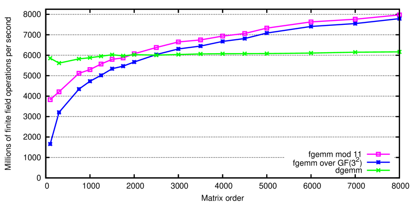
Figure 3: Speed of finite field Winograd matrix multiplication on a XEON, 3.6 GHz

Figure 4 shows only the speed of the conversion after the floating point operations. The log scales prove that for $q$ ranging from $2^{1}$ to $2^{26}$ (on a 32 bit Xeon) our new implementation is two to three times faster than the previous one.

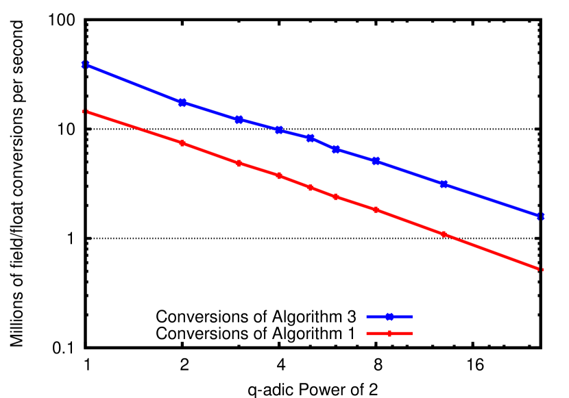
Figure 4: Small extension field conversion speed on a Xeon 3.6GHz

Furthermore, these improvements e.g. allow the extension field routines to reach the speed of 7800 millions of $\mathtt{GF}(9)$ operations per second (on a XEON, 3.6 GHz, using Goto BLAS-1.09 dgemm as the numerical routine [8] and FFLAS fgemm for the fast prime field matrix multiplication [6]) as shown on figure 3. The FFLAS routines are available within the LinBox 1.1.4 library [11] and the FQT is in implemented in the givgfqext.h file of the Givaro 3.2.9 library [3].

With these new implementations, the obtained speed-up shown in figure 3 represents a reduction from the 15 percent overhead of the previous implementation to less than 4 percent now, when compared to $\mathtt{GF}(11)$.

8 Conclusion

We have proposed a new algorithm for simultaneous reduction of several residues stored in a single machine word. For this algorithm we also give a time-memory trade-off implementation enabling very fast running time if enough memory is available.

We have shown very effective applications of this trick for both modular polynomial multiplication, and extension fields conversion to floating point. The latter allows efficient linear algebra routines over small extension fields but also linear algebra over small prime fields as shown in [2].

Further improvements include comparison of running times between choices for $q$. Indeed our experiments were made with $q$ a power of two and large table lookup. With $q$ a multiple of $p$ the table lookup is not needed but divisions by $q^{i}$ will be more expensive.

It would also be interesting to see how does the trick extend in practice to larger precision implementations: on the one hand the basic arithmetic slows down, but on the other hand the trick enables a more compact packing of elements (e.g. if an odd number of field elements can be stored inside two machine words, etc.).

References

- [1] Jean-Guillaume Dumas. Efficient dot product over finite fields. In Victor G. Ganzha, Ernst W. Mayr, and Evgenii V. Vorozhtsov, editors, Proceedings of the seventh International Workshop on Computer Algebra in Scientific Computing, Yalta, Ukraine, pages 139–154. Technische Universität München, Germany, July 2004.
- [2] Jean-Guillaume Dumas, Laurent Fousse, and Bruno Salvy. Compressed modular matrix multiplication. In Proceedings of the Milestones in Computer Algebra 2008, Tobago, May 2008.
- [3] Jean-Guillaume Dumas, Thierry Gautier, Pascal Giorgi, Clément Pernet, Jean-Louis Roch, and Gilles Villard. Givaro 3.2.9: C++ library for arithmetic and algebraic computations, 2007. ljk.imag.fr/CASYS/LOGICIELS/givaro.
-
[4]
Jean-Guillaume Dumas, Thierry Gautier, and Clément Pernet.
Finite field linear algebra subroutines.
In Teo Mora, editor, Proceedings of the 2002 International
Symposium on Symbolic and Algebraic Computation, Lille, France, pages
63–74.
ACM Press, New York,
July 2002.
- [5] Jean-Guillaume Dumas, Pascal Giorgi, and Clément Pernet. FFPACK: Finite field linear algebra package. In Jaime Gutierrez, editor, Proceedings of the 2004 International Symposium on Symbolic and Algebraic Computation, Santander, Spain, pages 119–126. ACM Press, New York, July 2004.
- [6] Jean-Guillaume Dumas, Pascal Giorgi, and Clément Pernet. Dense linear algebra over prime fields. ACM Transactions on Mathematical Software, 2009. to appear.
- [7] Joachim von zur Gathen and Jürgen Gerhard. Modern Computer Algebra. Cambridge University Press, New York, NY, USA, 1999.
- [8] Kazushige Goto and Robert van de Geijn. On reducing TLB misses in matrix multiplication. Technical Report TR-2002-55, University of Texas, November 2002. FLAME working note #9.
- [9] Vincent Lefèvre. The Euclidean division implemented with a floating-point division and a floor. Technical report, INRIA Rhône-Alpes, 2005. http://hal.inria.fr/inria-00000154.
- [10] Vincent Lefèvre. The Euclidean division implemented with a floating-point multiplication and a floor. Technical report, INRIA Rhône-Alpes, 2005. http://hal.inria.fr/inria-00000159.
- [11] The LinBox Group. Linbox 1.1.4: Exact computational linear algebra, 2007. www.linalg.org.
- [12] B. David Saunders. Personal communication, 2001.
- [13] Victor Shoup. NTL 5.4.1: A library for doing number theory, 2007. www.shoup.net/ntl.