The notion of persistence applied to breathers in thermal equilibrium

Abstract

We study the thermal equilibrium of nonlinear Klein-Gordon chains at the limit of small coupling (anticontinuum limit). We show that the persistence distribution associated to the local energy density is a useful tool to study the statistical distribution of so-called thermal breathers, mainly when the equilibrium is characterized by long-lived static excitations; in that case, the distribution of persistence intervals turns out to be a powerlaw. We demonstrate also that this generic behaviour has a counterpart in the power spectra, where the high frequencies domains nicely collapse if properly rescaled. These results are also compared to non linear Klein-Gordon chains with a soft nonlinearity, for which the thermal breathers are rather mobile entities. Finally, we discuss the possibility of a breather-induced anomalous diffusion law, and show that despite a strong slowing-down of the energy diffusion, there are numerical evidences for a normal asymptotic diffusion mechanism, but with exceptionnally small diffusion coefficients.

1 Introduction

For a decade or so, a growing interest has been manifested for the so-called breather modes [1, 2]. Two factors have contributed mainly to this popularity. First, these localized excitations are generic in arrays of oscillators, provided that both nonlinearity and a certain amount of discreteness are features of the system [3]; as such, they are a priori ubiquitous in nature and have thus a certain universality. But it was shown also that systems where breather modes can be found could display a strong slowing down of the energy diffusion, leading apparently to anomalous subdiffusive behaviours reminiscent to glassy states [4]; it was recognized that the slowing down is intimately related to the existence of so-called pinned breathers [5, 6, 7]. The difficulty however has remained up to now to bind these two features beyond qualitative arguments, due to the fact that, in contrast with topologic solitons for instance, the breather modes do not possess a true identity as dynamical elementary excitations, what makes their very existence problematic in realistic situations where systems are at or close to equilibrium. In these cases, a “breather” stricto sensu does no longer exist, even if clear dynamical features akin to them are undoubtedly observable.

The aim of this paper is to show that the concept of persistence distribution can be a useful tool and give an insight into the “breathers” distribution in a thermal context. Several studies have been already devoted to that subject [5, 6, 7, 8], but they all faced the empirical nature of a breather at $k_{B}T\neq 0$, and were forced to circumvent the problem by ad hoc recipes. The persistence distribution allows to overcome this difficulty: instead of focusing on the problematic recognition of breathers among a thermalized chain, one integrates the time axis into the problem and study the trend a site has to stay above the mean energy level for a time arbitrary long, i.e. its ability to persist above (or below) its average. By this way, we give up a real extraction of a breather distribution, but catch really the main interesting property of these thermal “breathers”, that is their ability to make last abnormally an energy fluctuation.

For a stochastic process $X(t)$, the persistence distribution $\mathcal{P}_{\pm}(\tau)$ is defined as the probability that the process stays above ($\mathcal{P}_{+}$) or below ($\mathcal{P}_{-}$) its mean value during the whole time interval $[0,\tau]$. This relatively simple definition hides a complicated observable, as $\mathcal{P}_{\pm}(\tau)$ assumes the knowledge of the whole dynamics from the time origin on[9]. We will show that this concept is particularly adapted to systems where thermal breathers are pinned, as they lead naturally to persistent local energy density: actually, the asymptotic branch of the persistence distribution can be taken as a definition of the thermal breathers distribution (see below). Besides, for systems where mobile thermal breathers are excited, the persistence distribution yields naturally a measure of the lifetime of the static entity created by the collisions of two breathers.

In this paper, we focus on discrete Klein-Gordon lattices described by the Hamiltonian

$$\mathcal{H} =\sum_{i}e_{i}$$ (1)

$$e_{i} =\frac{1}{2}\dot{x}_{i}^{2}+V(x_{i})+\frac{k}{2}x_{i}(2x_{i}-x_{i+1}-x_{i-1})$$

The dynamics of the lattices is exclusively microcanonical, and the temperature is extracted by the usual ensemble equivalence. As we are interested in the role of thermal breathers, we study systems which are close to the anticontinuum limit, that is $k/\omega_{0}^{2}\ll 1$, where $\omega_{0}^{2}$ is defined through $V(x)=C^{t}+\frac{1}{2}\omega_{0}^{2}(x-x_{\text{min}})^{2}+o(x-x_{\text{min}})^{2}$; in the following we take $k/\omega_{0}^{2}=0.1$.

As regards the on-site potentials $V(x)$, we have considered the hard $\phi^{4}$ potential $V_{1}(x)=\frac{1}{2}x^{2}+\frac{1}{4}x^{4}$ (famous for its pinned breathers), a soft potential $V_{2}(x)=\frac{1}{3}\log\cosh(\sqrt{3}x)$ (with a Taylor expansion $V_{2}(x)=\frac{1}{2}x^{2}-\frac{1}{4}x^{4}+o(x^{4})$; this potential has typically mobile thermal excitations) and the harmonic potential $V_{3}(x)=\frac{1}{2}x^{2}$. Note that $\omega_{0}^{2}=1$ in all these cases.

In a first part, we introduce the distribution of time intervals of persistent energy excess (TIPEE) $P(t)$ (closely related to the persistence), and discuss the numerical results for $P(t)$ for the three on-site potentials. We then study the power spectrum associated to these models and show some connections with the persistence behaviours. Next, we discuss the possibility of an anomalous diffusion for nonlinear Klein-Gordon with hard anharmonicity. Finally, we introduce the phenomenological concept of breather lifetime, and show that for static breathers of moderate-to-high energies, these lifetimes are exponentially increasing with their energy.

2 The TIPEE and persistence distributions

The time interval of persistent energy excess $P(t)$ is defined for positive and negative $t$. For positive $t$ (resp. negative), it is the distribution function of the time intervals during which a given site has its energy $e_{i}$ greater (resp. lower) than the mean local energy $\langle e_{i}\rangle$. It is very simple to measure, but actually this is a rather complicated statistical concept, just like the persistence distributions [9]. By the way, $P(t)$ is closely related to the persistence distributions above and below the mean energy by the relations (see Appendix) $\mathcal{P}_{\pm}(\tau)=\int_{\tau}^{\infty}dtP(\pm t)(t-\tau)/\int_{0}^{\infty}dt\ tP(\pm t)$. In the litterature of stochastic processes, the persistence distribution is widely used, but actually for our purpose, the TIPEE distribution $P(t)$ is more appropriate : we’ll focus on it henceforward.

To get $P(t)$ we must compulsorily perform numerical simulations : it is an object so complicated from the statistical point of view, that it is likely that no exact calculation would be amenable even for the integrable harmonic chain $V(x)=V_{3}(x)$.

2.1 Harmonic chain $V(x)=V_{3}(x)$

The numerical result for $P(t)$, plotted in figure 1,

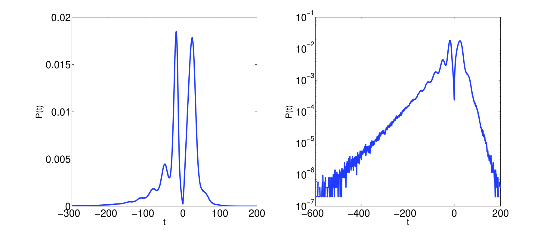
Figure 1: Distribution $P(t)$ for the harmonic potential $V_{3}(x)=\frac{1}{2}x^{2}$. Left : linear-linear plot; right : semilog plot.

is independent of the temperature, due to the invariance of the dynamics under a dilatation $(x,v)\rightarrow(\lambda x,\lambda v)$. The two main peaks that characterize the distribution give the typical times of a fluctuation; one easily verifies that they are of the same order of magnitude as $1/k$: a wave packet travels at $v_{g}$ throughout the system and is likely to create a positive fluctuation at a given site for a time or order $1/v_{g}\sim 1/k$. As regards the tails of the distribution, the two asymptotic branches of $P(t)$ have exponential relaxations, whence one can extract two characteristic times: $\tau_{-}\sim 57$ and $\tau_{+}\sim 16$, associated to rare events.

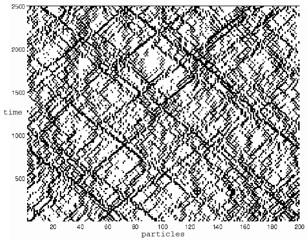
Figure 2: Hypsometric plot of the energy density for the harmonic system: sites with an energy above (resp. below) the mean value are black (resp. white).

These times are the quantitative traduction of what the eyes can observe in an hypsometric plot like that of fig 2: the sites experiencing long depletions of energy are related to rather large white patches of fig. 2; the quite large characteristic time $\tau_{-}$ tells us that the occurence of large patches of that kind are not so rare. On the contrary, a stagnant excess of energy is much more unlikely due to the group velocity which generically moves the wave crests; only for colliding wave crests can occur a long stagnation, but this is rare. All these features can be viewed as emergent properties of the phonon dynamics with stochastic initial conditions. The intrinsically rich nature of the persistence concept probably prevents a theoretical calculation, despite the fact that the system is integrable.

2.2 Soft potential $V(x)=V_{2}(x)$

For a soft potential like $V_{2}(x)$, moving breathers are expected. They must lead to a TIPEE distribution not qualitatively different from the preceding case. This is almost the case, as figure 3 shows.

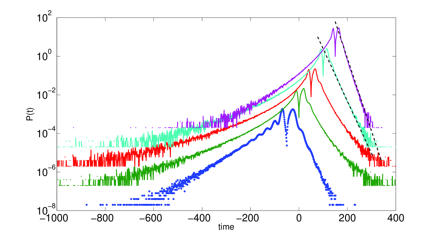
Figure 3: Distribution $P(t)$ for the soft potential $V_{2}(x)$ at various temperatures. From bottom to top : harmonic potential (i.e. $V_{2}$ for $k_{B}T\rightarrow 0$), $k_{B}T=0.25$, $k_{B}T=0.5$, $k_{B}T=1.0$, $k_{B}T=2.0$. The curves were shifted in both directions for sake of clarity.

The distribution depend now on the temperature, and the exponential tails are still present except near the temperature $k_{B}T=0.25$. This temperature corresponds to a minimum in the diffusion coefficient, a minimum resulting from the simultaneous destruction of the phonon structure by the nonlinearity and the excitations of rather static breathers (see figure 4, left panel). Actually, for the $V_{2}$ potential, the mobility of breathers is an increasing function of their energy (or the temperature). The static breathers perturbs the picture of mobile entities passing in a finite time through a particular site, colliding into each other, etc…, and this perturbation leads to nonexponential tails in the TIPEE distribution.

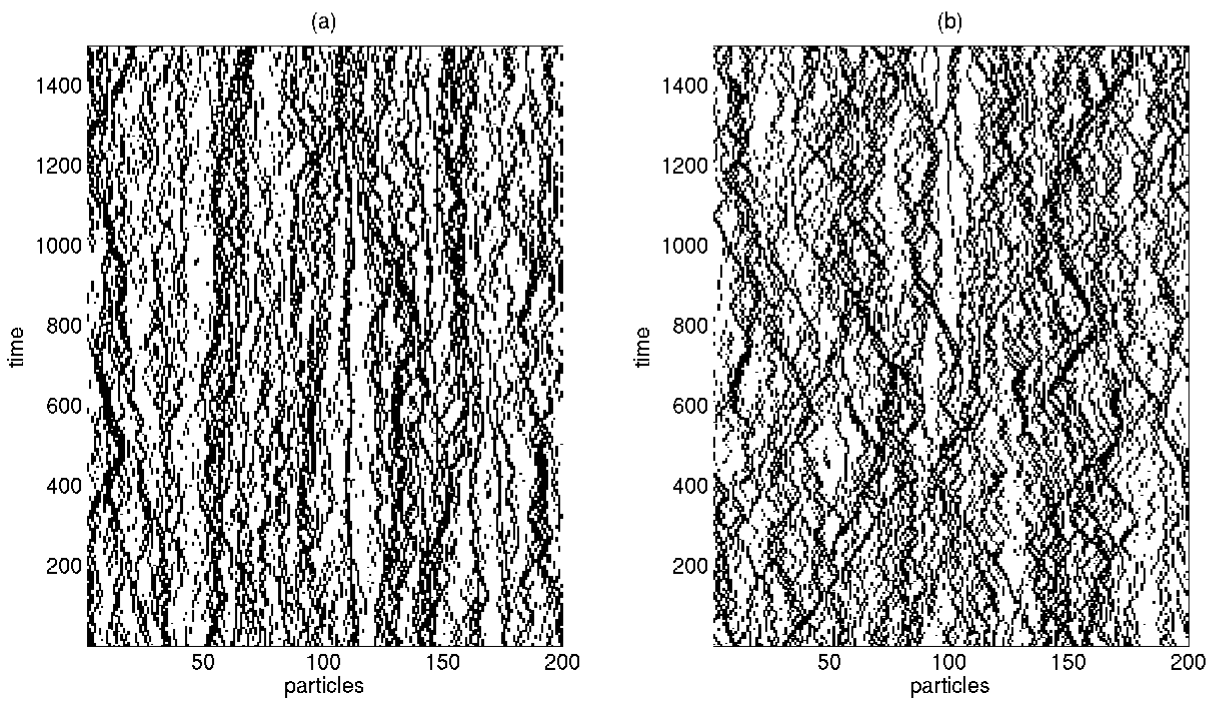
Figure 4: Hypsometric plot of the energy density for the potential $V_{2}(x)$. Left: $k_{B}T=0.25$, right: $k_{B}T=2.0$. The temperature $k_{B}T=0.25$ corresponds to the minimum value of the diffusion coefficient.

These nonexponential tails anticipate the behaviour of the potential $V_{1}(x)$, where static breathers are the rule rather than the exception. Here, by increasing the temperature, the thermal breathers become mobile (see fig. 4 right panel) and the exponential tails are restored in the distribution: this is indicated in figure 3 by the dotted lines added to the curves for $k_{B}T=1$ and $k_{B}T=2$. On the contrary, the exponential behaviour is not restored on the left wing of the distribution: the rare occurence of lasting depletions is “less rare” than in the harmonic case, probably due to the fact that the calm regions have frequencies detuned with those of breathers, and thence can act as reflective barriers for them, lengthening their lifetime. Such a scenario can be clearly observed on the right panel of fig. 4 (near particles numbered 100 and 180).

2.3 Hard potential $V(x)=V_{1}(x)$

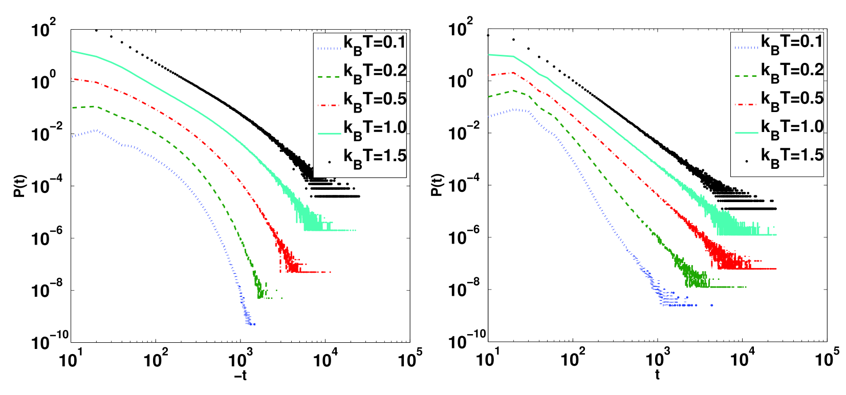
Figure 5: Distribution $P(t)$ for the hard potential $V_{1}(x)=\frac{1}{2}x^{2}+\frac{1}{4}x^{4}$ at various temperatures. Left panel: negative times, right panel: positive times. The curves were shifted in vertical direction for sake of clarity.

For the hard potential $V_{1}(x)=\frac{1}{2}x^{2}+\frac{1}{4}x^{4}$, a remarkable feature emerges for positive $t$ (see fig 5, right panel) : except for very low $T$, where the system resembles the harmonic system, the asymptotic tail is clearly a powerlaw: no characteristic time is associated to long lasting breathers, which assume surprisingly this simple distribution law. Why this is so is not easy to understand, as it is related to the local structure of the dynamical phase space, but a phenomenological model can be attempted. Let us assume that the energy $\varepsilon$ of a given site obeys a simple Fokker-Planck equation; owing to the equilibrium distribution $P_{eq}(\varepsilon)\propto\exp(-\beta\varepsilon)$ (we neglect the entropic contribution of the phase degree of freedom), it reads

$$\partial_{t}p=\frac{1}{2}\frac{\partial}{\partial\varepsilon}\left[B(\varepsilon)[\beta p+\partial_{\varepsilon}p]\rule[-1.94444pt]{0.0pt}{8.88889pt}\right]$$ (2)

where $\beta=1/k_{B}T$ and $B(\varepsilon)$ is an unknown diffusion coefficient. This modelling is rather crude, as it disregards completely the conserved character of the energy as well as the extended nature of the system. The diffusion coefficient $B(\varepsilon)$ is a priori unknown, but we know that it is a decreasing function of the energy. The simplest Ansatz we can make is to choose $B(\varepsilon)\propto\exp(-\nu\varepsilon)$, where $\nu$ is a positive coefficient. According to a procedure described in [10], one can derive the asymptotic behaviour of the persistence distribution. In that case, it yields an appealing result, namely a temperature dependent powerlaw :

$$\mathcal{P}_{+}(t) \propto\frac{1}{t^{1+\beta/\nu}}$$ (3)

$$\Longrightarrow P(t) \propto\frac{1}{t^{3+\beta/\nu}}$$ (4)

Thus, the exponential Ansatz for $B(\varepsilon)$ seems reasonable, but we could also attempt a powerlaw Ansatz $B(\varepsilon)\propto 1/\varepsilon^{\mu}$. The same demonstration from [10] yields

$$\mathcal{P}_{+}(t)\propto t^{-\frac{\mu-1}{2\mu+2}}\times\exp[-(t/t_{0})^{1/(1+\mu)}]$$ (5)

which is clearly not appropriate here.

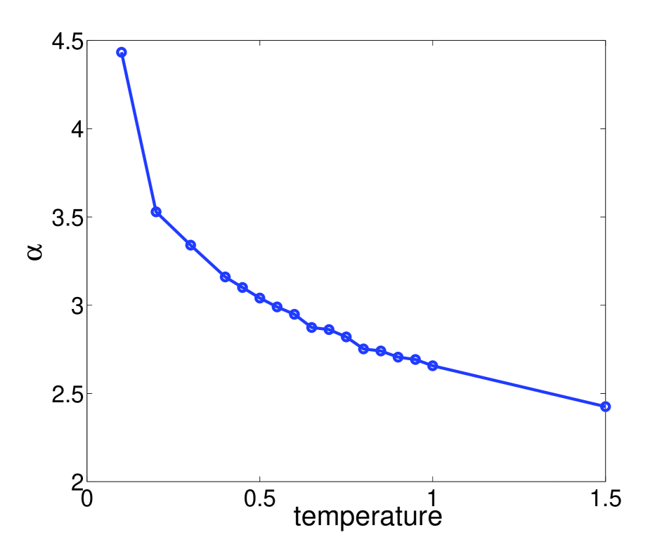
Figure 6: Exponent $\alpha$ associated to $P(t)$ for the potential $V_{1}$. $\alpha$ is defined by $P(t)\propto 1/t^{\alpha}$ for large positive $t$

So far so good, it seems from (4). Actually, the result is not that good: to see that, we extract from the curves in figure 5 (right panel) the exponents for each temperature. They are plotted on figure 6, and it is clear that the exponent is overestimated by this simple approach: the actual exponent is lower than 3 for high $T$, which is not possible in the Fokker-Planck approach. The positive point is that the temperature dependence is qualitatively similar, i.e. the temperature lowers the exponent (the curve is however not described by $C^{t}+C^{t^{\prime}}/T$). One could argue the problem could be solved by choosing a kernel $B$ decreasing much faster for high $\varepsilon$. But one can show that for $B(\varepsilon)\propto\exp(-\nu\varepsilon^{1+\eta})$, one has asymptotically $\mathcal{P}_{+}(t)\propto 1/t$ irrespective of the values of $\nu$ and $\eta>0$.

A possible explanation for these disagreements is to be traced back to the fact that the Fokker-Planck approximation for the energy diffusion is a markovian one, which is a rather poor assumption for pinned thermal breathers in 1D : they are so to speak squeezed in between two other breathers which act as reflecting barriers for the mobile phonons and prevent a rapid decorrelation of the noise. This too slow evolution of the thermal degrees of freedom slows the degradation of the breathers and give them a longer persistence. To conclude, the inability of that simple model to quantitatively account for the phenomenology tells us that the giant slowing down experienced by the system is not only due to an effective diffusion coefficient in the energy space (the kernel $B(\varepsilon)$) which would decrease for increasing energy, but that the geometrical constraints, squeezing in each breather between two other breathers give a marked non markovian character to the dynamics and therefore plays a prominent role to the overall slowing down. But, why the persistence distribution of the breathers is powerlaw for model $V_{1}$ remains an interesting unsolved question.

3 The power spectrum

It is useful to have a look at the adimensionate power spectrum $S(\omega)$ defined by $\langle v_{i}^{*}(\omega^{\prime})v_{i}(\omega)\rangle=k_{B}TS(\omega)\delta(\omega-\omega^{\prime})$ where $v_{i}(\omega)$ is the Fourier Transform of $v_{i}(t)$. Roughly speaking, $S(\omega)$ gives the frequency content of the local thermal excitations, and in principle should bear a trace of the thermal “breathers”.

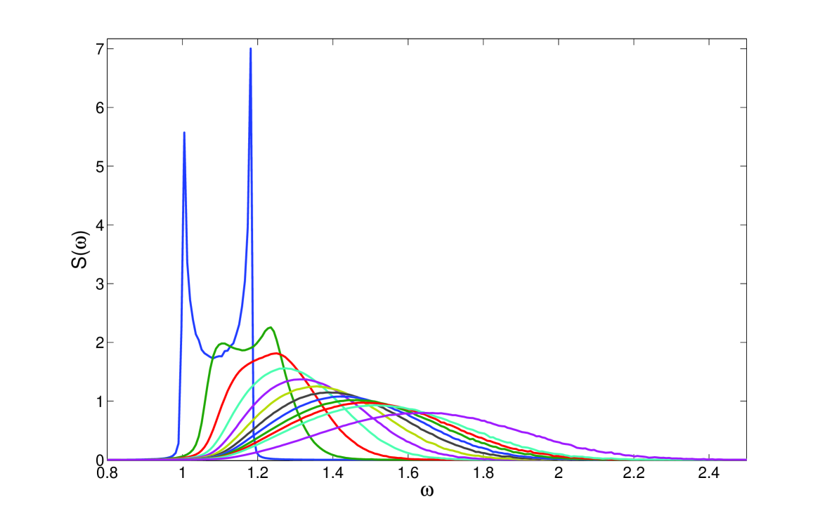
Figure 7: Power spectrum $S(\omega)$ for various temperatures : from left to right, harmonic system ($T\rightarrow 0$), $T=0.1(0.1)1.0$ and $T=1.5$.

The power spectrum for the potential $V_{1}$ is plotted in figure 7 for various temperatures (notice that the curve for $T\sim 0$ corresponds to the harmonic potential $V_{3}$) . The global shift of the spectra to the right for increasing temperature is obviously due to the “hard” features of the potential: for a single oscillator, the frequency increases with the particle energy. It is remarkable that no blatant evidences of the breathers can be isolated, like peaks growing outside the phonon band for instance, a fact already noticed previously [8]. This is due to the fact that breathers of various energies are stable without restriction above the upper bound of the phonon band.

However, one expects that for temperatures high enough, at least the right asymptotic of the spectra (the part rightwards the maximum) accounts for breathers. As the distribution of breathers, or more precisely, the distribution of their persistence, is powerlaw, and retains this shape for various temperatures, one expects these right wings to be more or less universal.

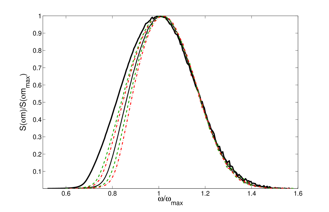
Figure 8: Rescaled power spectra $S(\omega)/S(\omega_{max})$ as a function of $\omega/\omega_{max}$ for various temperatures : from left to right, $T=1.5,1.0,0.9,0.8,0.7,0.6$

Figure 8 represents various power spectra from $k_{B}T=0.6$ to $k_{B}T=1.5$ where the axis were stretched so that the maxima of the curves coincide at $(1,1)$ (we allowed also an extra small horizontal translation of at most $5.10^{-2}$ to allow for the numerical uncertainty of the position of the maximum). The figure shows clearly that the right side of the curve can be described by the same master curve, provided the temperature is not too low (for $k_{B}T\leqslant 0.5$ we observed a noticeable departure from the collapsed right branch). On the contrary, the left branches do not collapse on a single curve but stretch to the left for increasing temperatures. This is related to the fact that the ratio $\Delta\omega/\omega_{max}$, where $\Delta\omega$ is the frequency width of $S(\omega)$ and $\omega_{max}$ its maximum, increases with the temperature.

It is not uninteresting to have a look at the power spectra associated with the soft potential $V_{2}$ (see fig 9).

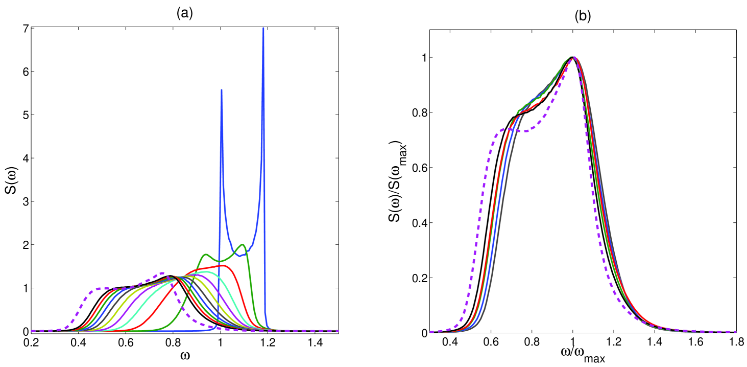
Figure 9: Natural (a) and rescaled (b) power spectra for the potential $V_{2}$ and for various temperatures. For (a) : from right to left, $k_{B}T=0(0.1)1.0,1.5$. For (b) $k_{B}T=0.6(0.1)1.0,1.5$. For sake of clarity, the curve corresponding to $k_{B}T=1.5$ has been dashed in both plots.

As expected, the power spectra shift toward low frequencies when temperature is increased. Moreover, as already noticed with the persistence distribution, high temperatures restore an effective phonon behaviour, which is embodied here by the bimodal structure of the curve, shaded for intermediate $k_{B}T$ but restored for higher $k_{B}T$. Finally, the same rescaling as in figure 8 (in fig. 9 (b)) does not highlight any collapse as for $V_{1}$: this confirms indirectly the intimate relation between the collapse of fig. 8 with the thermal static breathers.

4 Anomalous or normal diffusion ?

A natural question raises when considering the system with the potential $V_{1}$. The nucleation of pinned breathers which besides reflects efficiently the phonons (by the frequency detuning), affects deeply the diffusion properties of the system; does it induce a qualitative change toward an anomalous subdiffusive behaviour ? The numerical results as those of [4] suggest that it is indeed the case, but their numerical experiments are to some extent “extremely” out of equilibrium near the boundaries, leading to a enormous detuning; as far as I know, the normality of the energy diffusion has not been tested at equilibrium. For a system having a normal energy diffusion, the autocorrelation of the energy density must behave $\propto 1/\sqrt{t}$ at large times. This is for instance the case for the system with the potential $V_{2}$, as shown in figure 10; in that figure,

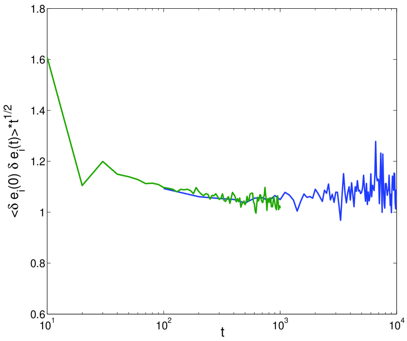
Figure 10: For the potential $V_{2}$, (energy density autocorrelation function)x(square root of time) as a function of time. The two curves probe the same system at different time ranges ($k_{B}T=1$).

the autocorrelation of energy $\langle\delta e_{i}(0)\delta e_{i}(t)\rangle$ is multiplied by $\sqrt{t}$, in order to get a plateau for a normal diffusive behaviour. In figure 10, this plateau is unmistakable, despite unavoidable fluctuations due to a lack of statistical accuracy. Now let us consider the system with the hard potential $V_{1}$. The figure 11 is the same as fig. 10, except that the potential is $V_{1}$ (and the plot is log-log).

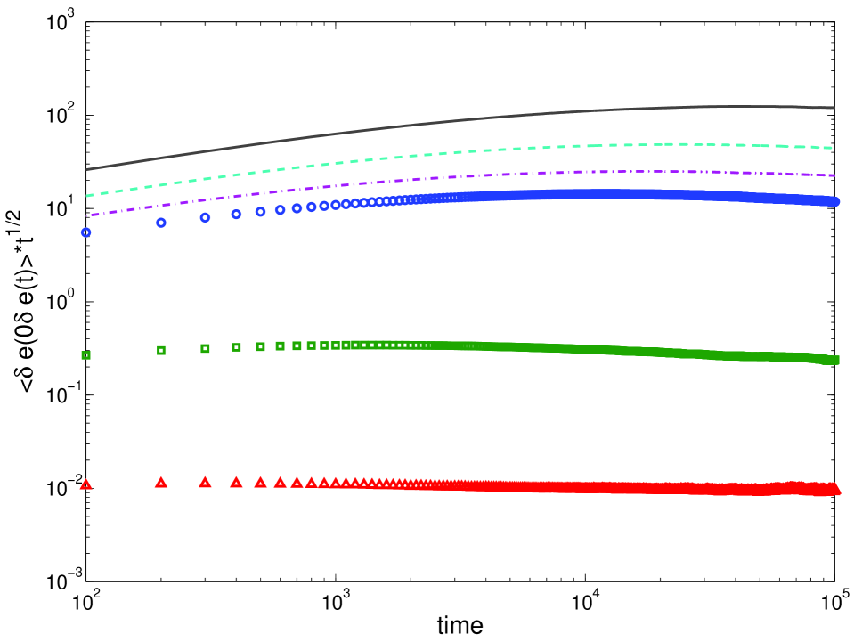
Figure 11: For the potential $V_{1}$, (energy density autocorrelation function)x(square root of time) as a function of time. The different curves correspond to temperatures $k_{B}T$=0.1 (triangles), 0.3 (square), 1.0 (circles), 1.2 (dash-dot), 1.5 (dashed), 2.0 (solid).

Clearly, for low temperatures, the system displays a normal diffusive behaviour. For higher temperatures, the slowing down induced by the thermal breathers makes the curves increase higher the higher $k_{B}T$, but for each curve computed, this increase ceases and the curves have a maximum. It would be difficult numerically to probe these curves for longer times, but we think that the figure 11 shows convincingly that the ultimate regime of relaxation for the system is a normal one: obviously, the curves cannot decrease to zero: it would lead to a superdiffusive behaviour which is physically absurd; thus, it is most probable that these curves reach eventually a plateau regime, but it is worth stressing that this ultimate regime is extremely remote for high temperatures: for $k_{B}T=1.5$ or $2$, at $t=10^{5}$, the system has not reached its asymptotic regime. Thus, in that kind of system, the pinned thermal breathers do not modify the very nature of the energy diffusion, but slow down enormously the diffusion: as a result, the signature of thermal breathers one can get not only in the very small values of the diffusion coefficients, but also in the very long transients observable in the correlation functions of the energy density. But this study indicates that it is not correct to see a system with breathers as a vitreous system, as at equilibrium there is no indication that anomalous diffusion takes place, not to mention ergodicity breaking.

5 Breather lifetime

As we have already stressed, “breathers” as numerable entities do not exist for generic states of the system. However, for the system with the hard potential $V_{1}$, the hypsometric plots [4] show clearly that for not too low $k_{B}T$, the eye can separate without much ambiguity different excitations, almost static, which it is tantalising to term “breathers”. Thus, in that case, a phenomenological approach based on an effective population of breathers is not meaningless, and it is interesting to confront that approach to the results we have got for the persistence. In the following we consider only the model $V_{1}$.

We assume that the energy into the system is dispatched amongst $N_{b}$ breathers. The distribution of the free energies is taken $p(E)\propto\exp(-\beta E)$, what is slightly uncorrect, as the entropic degrees of freedom (associated to the phase coordinate of the breathers) are neglected; but for sake of simplicity, we retain this exponential law. In principle, the number $N_{b}$ can be related to the number $N$ of particles via the formula $N_{b}\langle E\rangle=N\langle e_{i}\rangle$, but for $k\rightarrow 0$, one has $N_{b}\approx N$.

These $N_{b}$ breathers are essentially static excitations with long lifetimes. We can assume that the right tail of the distribution $P(t)$ is entirely constructed by these breathers. As the lifetime of a breather is obviously an increasing function of its energy, we can write $P(t)dt\propto p(E)dE$. Thus, for high energies, $dt/t^{\alpha}\propto\exp(-\beta E)dE$, whence one deduces the lifetime of a breather as a function of its energy :

$$t(E)\propto\exp\left(\frac{\beta E}{\alpha-1}\right)$$ (6)

These lifetimes are thus exponentially related to the energies, what is reminiscent of an Arrhenius law. It is probably quite bold or even incorrect to surmise that the decay of a breather is an activated process, as it is clear that no Peierls-Nabarro barrier does exist for breathers; anyway, a barrier can be sometimes entirely due to entropic effects, namely, the shift of a breather from one site to an adjacent one (what is, owing to the definition of the persistence, equivalent to the “death” of a breather at his starting site) could occur without energy changes but through a succession of different states so tailored that it makes an effective entropic barrier. Thus, if we follow this line, the effective depth of the local well where the system oscillates when a breather of energy $E$ exists would be given by $E/(\alpha-1)$ : the depth is proportionnal to the energy of the excitation but lower than it; it is temperature dependent, and tends to increase with increasing $T$ ($E$ being fixed).

To proceed further, it would be necessary to study carefully the multidimensional phase space of these systems (and the corresponding dynamics), to see if the theory of dynamical systems can give more consistency and support to these phenomenological remarks.

6 Conclusion

In this paper, we have studied different Klein-Gordon chains at thermal equilibrium. These systems possess breather solutions of the Hamiltonian dynamics, which can be considered as periodic excitations at zero temperature. At $k_{B}T\neq 0$, the concept of breather is void in principle, but transient local maxima of energies which behave like individual items can be observed in these systems near the anticontinuum limit, which are termed thermal breathers by extension. We have shown that the concept of persistence is well adapted to study these objects when they are firmly pinned as in most of Klein-Gordon chains with hard nonlinear potentials. Interestingly enough, the persistence distributions are asymptotically powerlaw, with an exponent decreasing with the temperature. This remarkable feature has been shown to be intimately related to both the geometrical structure of the phase space and the non markovian character of the local dynamics. But the very explanation of this “multifractal” distribution in terms of dynamical systems remains an open issue. Moreover, we have also shown that this particularly simple distribution of breathers of high energies has a translation in the power spectra : using axis rescaling to superimpose the maxima, it turned out that the high frequency tails of the distributions coincide exactly, witnessing that a certain universality —some would term it perhaps “self-organized criticality”— is at work in the dynamics of breathers, provided the temperature is high enough to have destroyed completely the phonon structure.

This work raise some other issues: for discrete nonlinear systems in 2d or 3d, what tell the persistence or TIPEE distributions ? Clearly, the topology is much less a constraint, and the slowing down of the energy diffusion is less pronounced; but it would be interesting to test if the thermal breathers affect sensibly the persistence distributions, yielding for instance nonexponential asymptotic tails. Another issue is related to systems like model $V_{2}$: clearly for systems where the thermal “breathers” are mobile, following the persistence of a given site is not the ideal way of having signatures of breathers. The natural idea would be to define an extended persistence concept, allowing to follow a positive fluctuation of energy from one site to an adjacent one. This idea is appealling, but hides a certain number of technical difficulties related to the fact that instead of following a site, one follows a positive fluctuation: one implicitely tries to extract a breather distribution with all the ambiguities associated to it.

7 Appendix: Relation between TIPEE and persistence

Let us consider a large time interval $[0,T]$, when a stochastic process $Y(t)=X(t)-\langle X\rangle$ perform a number of sign flips. The time interval divides in $N\gg 1$ time intervals $\tau_{1},\ldots,\tau_{N}$ where $Y$ keeps a constant sign, and $\tau_{i}$ is taken negative if $Y(t)<0$ on that time interval. The repartition function of the $\tau_{i}$ is nothing but the TIPEE (Time Intervals of Persistent Energy Excess) $P(\tau)$. We have in particular

$$\int_{-\infty}^{\infty}d\tau P(\tau)=1$$ (7)

The persistance above zero for $Y$ is defined as the probability $\mathcal{P}_{+}(\tau)$ that “$Y(t)$ stays above zero for a time longer than $\tau$, knowing it started from a positive value”. The probability that it started from a positive value is just $\left(\int_{0}^{\infty}dt\ tP(t)\right)/\left(\int_{-\infty}^{\infty}dt\ tP(t)\right)$. The probability that $Y(t)$ stays above zero for a time $>\tau$ and it started from a positive value, is associated to the chance we have to pick up at random a time in $[0,T]$, such that we are in a positive interval of length greater than $\tau$, and far enough from the end such that the condition is fulfilled. This probability is thus given by

$$\int_{\tau}^{\infty}d\tau^{\prime}\left(\frac{P(\tau^{\prime})\tau^{\prime}}{\int_{-\infty}^{\infty}d\tau^{\prime\prime}|\tau^{\prime\prime}|P(\tau^{\prime\prime})}\right)\times\frac{\tau^{\prime}-\tau}{\tau^{\prime}}$$ (8)

whence we get

$$\mathcal{P}_{+}(\tau)=\int_{\tau}^{\infty}d\tau^{\prime}\ P(\tau^{\prime})(\tau^{\prime}-\tau)\left/\int_{0}^{\infty}d\tau^{\prime}P(\tau^{\prime})\tau^{\prime}\right.$$ (9)

We verify that $\mathcal{P}_{+}(0)=1$. The corresponding formula for $\mathcal{P}_{-}(\tau)$ is readily obtained by changing $\tau$ by $-\tau$ in $P$.

References

- [1] S. Flach and C.R. Willis, Physics Reports,295, 181-264 (1998).
- [2] S. Aubry, Physica D,216,1-30 (2006).
- [3] R.S. MacKay and S. Aubry, Nonlinearity,7,1623-1643 (1994).
- [4] G.P. Tsironis and S. Aubry, Phys. Rev. Lett.,77 5225-5228 (1996).
- [5] R.Reigada, A.H.Romero, A.Sarmiento, K.Lindenberg, J.Chem.Phys.,111, 1373-1384 (1999).
- [6] M. Eleftheriou and S.Flach, Physica D, 202, 142-154 (2005).
- [7] M.V.Ivanchenko, O.I.Kanakov, V.D.Shalfeev, S.Flach, Physica D, 198, 120-135 (2004).
- [8] M. Eleftheriou, S. Flach and G. P. Tsironis, Physica D, 186,20-26 (2003).
- [9] S.Majumdar, Curr. Sci., 77 370 (1999).cond-mat/9907407
- [10] J.Farago, Europhys.Lett.,52, 379 (2000).