A Novel Solution to the ATT48 Benchmark Problem

Abstract

A solution to the benchmark ATT48 Traveling Salesman Problem (from the TSPLIB95 library) results from isolating the set of vertices into ten open-ended zones with nine lengthwise boundaries.  In each zone, a minimum-length Hamiltonian Path (HP) is found for each combination of boundary vertices, leading to an approximation for the minimum-length Hamiltonian Cycle (HC).  Determination of the optimal HPs for subsequent zones has the effect of automatically filtering out non-optimal HPs from earlier zones.  Although the optimal HC for ATT48 involves only two crossing edges between all zones (with one exception),  adding inter-zone edges can accomodate more complex problems.

1 Introduction

Given a set of vertices, the well-known Traveling Salesman Problem (TSP) involves finding the minimum-length Hamiltonian Cycle (HC): the path visiting each vertex once and returning to the starting vertex.

The symmetric TSP with $N$ vertices has $(N-1)!/2$ permutations, precluding an exhaustive search except for small $N$. Even a relatively small problem (e.g., $N=20$) has $10^{16}$ distinct HCs; $N=40$ leads to $10^{46}$ distinct HCs. The Euclidean TSP is classified as an NP-hard problem¹, having no known algorithm for the general case whose number of operations is a polynomial function of $N$.

The $(N-1)!/2$ permutations assume that any vertex can occupy any of $N$ positions. Isolating vertices into spatial zones locks each into a limited range of positions, subject to boundary vertex permutations.  This falls into the general area of dynamic programming^2,3,4.

Partitioning the vertices into sub-problems has been done for the Euclidean TSP^5-10. In particular, Arora⁶ obtained a Polynomial Time Approximation Scheme (PTAS) generating a tour exceeding the optimal length by no more than a factor of $1+\varepsilon$ in time $N^{O(1/\varepsilon)}$. The approach involved a bounding square box dissected into squares and shifted randomly, with restrictions on edge crossings (to specified portals).  Mitchell⁷ independently obtained a similar result.

The approach in this paper dissects the problem lengthwise and finds optimal Hamiltonian Paths (HPs)—paths visiting each vertex once—for the isolated zones independently of the others. The number of combinations of boundary vertices determines the number of optimal HPs for each zone.  Sets of optimal HPs for each zone (with embedded HPs from previous zones) generate an HC for the set of vertices.  When no boundary vertices are omitted, the optimal HC will contain an optimal HP found from each zone.

This paper illustrates the procedure for a benchmark problem (i.e., ATT48¹¹) small enough to permit a detailed description of the entire solution process. The success of the approach depends on limiting the number of potential boundary vertices and crossing edges.  In practice, sometimes as few as two edges will cross a boundary from one zone to another.  The number of crossing edges can be increased, if necessary, to improve the solution.

2 Outline of the Approach

Following previous approaches^5-10, the problem is broken down into subproblems that depend on each other through boundary interactions. The boundaries have a lengthwise nature, forming (doubly) open-ended zones. Figure 1 shows the separation of the ATT48¹¹ vertices into ten zones by means of nine introduced boundaries, each dissecting the problem lengthwise. Table 1 summarizes the zones and potential boundary vertices for each. Each zone connects to adjacent zones via a limited number of edges. (An edge is a straight line connecting two vertices.)

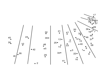
Figure 1: Separation of the ATT48 vertices into ten open-ended zones

A single lengthwise boundary cuts the optimal HC into an even number of HPs, the sum of which must have the minimum length in each of the two created spatial zones. For example, if two HPs are created, the HP in each created zone (terminated at boundary vertices in the other zone) must have the minimum length. If an HP length exceeds the minimum, replacing it with another HP (having the same vertices) will reduce the overall HC length.  Stated another way, it is not possible to dissect the optimal HC into two HPs and replace one of them with a shorter HP having the same vertices.

The boundary vertices contained by the optimal HC associated with a particular dissection are in general not known, requiring the enumeration of all possible boundary vertices located in the adjacent zone.  Typically, not all potential boundary vertices will connect edges to the adjacent zone. For example, as few as two edges ($n=2$) might connect two zones.  For each value of $n$, the binomial coefficient $\left(\begin{array}[c]{c}b\\ n\end{array}\right)$ provides the number of boundary vertex combinations ($b$ is the number of potential boundary vertices).  Summing over all values of $n$ leads to $2^{b-1}-1$ combinations (when $n=0$ and odd values of $n$ are eliminated).  A minimum-length HP is then found for each particular boundary vertex combination, beginning at the left end zone in figure 1 (zone 1).

The second boundary from the left in figure 1 isolates both zones 1 & 2 from the other vertices. The approach then finds the set of minimum length HPs for the combined vertices in zones 1 & 2 in the same way, except that the previously determined HPs from zone 1 become embedded in the new HPs.

Boundary vertices can comprise all the vertices in the adjacent zone, or (more likely) a smaller subset, usually those closest to the boundary. Vertices close to the boundary often have the effect of eliminating other potential boundary vertices because the latter often lead to non-optimal HCs.

Table 1. ATT48 Zones and Boundary Vertices

Zone	Vertices	Potential Boundary Vertices
$1$	$4,35,45$	$26,10,24$
$2$	$26,10,24$	$2,29,42,48,39,32$
$3$	$2,29,42,5,48,39,32$	$41,34,14,25,13,21$
$4$	$41,34,14,25,13,21$	$16,22,3,23,11,47$
$5$	$16,22,3,23,11,47$	$8,1,9,40,15,12,20$
$6$	$8,1,9,40,15,12,33,20$	$38,31,46,44,36$
$7$	$38,31,46,44,18,7,36$	$28,6,30$
$8$	$28,6,30,37,19$	$27,43$
$9$	$27,43$	$17$
$10$	$17$	—–

The set of minimum-length HPs found for each zone (combined with all previously-considered zones) includes embedded HPs from the previous zones.  However, as the approach determines HPs for later zones, it automatically begins to filter out non-optimal embedded HPs from previous zones, until at the last zone, $n=b=2$, and no extraneous HPs remain.

3 Detailed Description of the Solution

When the introduced boundaries create zones with boundary vertices confined to the adjacent zones, the sets of candidate HPs are found by advancing one zone at a time, considering only the vertices in the zone in question (with embedded HPs from previous zones) and its adjacent zone to the right.

The zone 1 vertices (4, 35, & 45) can connect to two of the three boundary vertices in zone 2 via inter-zone edges according to one of three combinations: 10 & 26, 26 & 24, or 10 & 24.  Determination of minimum-length HPs involves evaluating all interior vertex permutations for each of the three boundary vertex combinations.  Table 2 shows the results.

Table 2. Candidate HPs for zone 1

$\ 26$	$\ \ 4$	$\ 35$	$\ 45$	$\ 10$
$\ 26$	$\ \ 4$	$\ 35$	$\ 45$	$\ 24$
$\ 10$	$\ \ 4$	$\ 35$	$\ 45$	$\ 24$

Introduction of the second boundary leads to the determination of HPs for the combined vertices in zone 1 and zone 2 (i.e., vertices 26, 10, & 24).  Each HP terminates to two (or more) of the boundary vertices 2, 29, 42, 48, 39, & 32. (Vertex 5 is effectively shielded by vertices 48 and 42.)  When $n=2$, the six boundary vertices in zone 3 have fifteen possible combinations. Although $n=4$ is possible, it would require two edges from vertex 10 to cross the boundary.  Including extra crossing edges would lead to the evaluation of more boundary vertex combinations, and would involve determining optimal HPs on the basis of the sum of their lengths (with embedded HPs from zone 1).

Table 3 shows the possibilities searched in zone 2 for the candidate HPs when $n=2$. Vertices $V_{1}$ and $V_{2}$ are two of the boundary vertices 2, 29, 42, 48, 39, and 32.  Embedded HPs (e.g., 10-24, 10-26, & 24-26) are shown in bold typeface, both in the text and in the tables.

Table 3. Zone 2 possibilities searched with embedded HPs from zone 1

$V_{1}$

$V_{1}$

$V_{1}$

$V_{1}$

$V_{1}$

$V_{1}$

$V_{1}$

$V_{1}$

$V_{1}$

$V_{1}$

$V_{1}$

$V_{1}$

$\boldsymbol{10}$

$\boldsymbol{24}$

$26$

$26$

$\boldsymbol{26}$

$\boldsymbol{24}$

$10$

$10$

$\boldsymbol{10}$

$\boldsymbol{26}$

$24$

$24$

$\boldsymbol{24}$

$\boldsymbol{10}$

$\boldsymbol{10}$

$\boldsymbol{24}$

$\boldsymbol{24}$

$\boldsymbol{26}$

$\boldsymbol{26}$

$\boldsymbol{24}$

$\boldsymbol{26}$

$\boldsymbol{10}$

$\boldsymbol{10}$

$\boldsymbol{26}$

$26$

$26$

$\boldsymbol{24}$

$\boldsymbol{10}$

$10$

$10$

$\boldsymbol{24}$

$\boldsymbol{26}$

$24$

$24$

$\boldsymbol{26}$

$\boldsymbol{10}$

$V_{2}$

$V_{2}$

$V_{2}$

$V_{2}$

$V_{2}$

$V_{2}$

$V_{2}$

$V_{2}$

$V_{2}$

$V_{2}$

$V_{2}$

$V_{2}$

Each of the twelve possibilities in table 3 are searched for the fifteen $V_{1}$/$V_{2}$ combinations to obtain fifteen minimum-length HPs for zone 2 (table 4), with embedded HPs in bold.  The zone 2 solution contains only embedded HPs 26-10 & 26-24, eliminating HP 10-24.

Table 4. Candidate HPs for zone 2

$2$	$\boldsymbol{26}$	$\boldsymbol{10}$	$24$	$29$
$2$	$\boldsymbol{26}$	$\boldsymbol{10}$	$24$	$42$
$2$	$\boldsymbol{26}$	$\boldsymbol{10}$	$24$	$48$
$2$	$\boldsymbol{26}$	$\boldsymbol{10}$	$24$	$39$
$2$	$\boldsymbol{26}$	$\boldsymbol{10}$	$24$	$32$
$29$	$\boldsymbol{26}$	$\boldsymbol{10}$	$24$	$42$
$29$	$\boldsymbol{26}$	$\boldsymbol{10}$	$24$	$48$
$29$	$\boldsymbol{26}$	$\boldsymbol{10}$	$24$	$39$
$29$	$\boldsymbol{26}$	$\boldsymbol{10}$	$24$	$32$
$42$	$\boldsymbol{26}$	$\boldsymbol{10}$	$24$	$48$
$42$	$\boldsymbol{26}$	$\boldsymbol{10}$	$24$	$39$
$42$	$\boldsymbol{26}$	$\boldsymbol{10}$	$24$	$32$
$48$	$10$	$\boldsymbol{26}$	$\boldsymbol{24}$	$39$
$48$	$10$	$\boldsymbol{26}$	$\boldsymbol{24}$	$32$
$39$	$10$	$\mathbf{26}$	$\mathbf{24}$	$32$

The zone 3 solution (table 5) has only two distinct embedded HPs:  2-42 & 32-42.  Table 4 shows that both contain the embedded HP 26-10 from zone 1.

Table 5.  Candidate HPs for zone 3

$41$	$29$	$2$	$\boldsymbol{42}$	$\boldsymbol{32}$	$39$	$48$	$5$	$34$
$41$	$29$	$\boldsymbol{2}$	$\boldsymbol{42}$	$5$	$48$	$32$	$39$	$14$
$41$	$29$	$\boldsymbol{2}$	$\boldsymbol{42}$	$5$	$48$	$32$	$39$	$25$
$41$	$29$	$\boldsymbol{2}$	$\boldsymbol{42}$	$5$	$48$	$39$	$32$	$13$
$41$	$29$	$\boldsymbol{2}$	$\boldsymbol{42}$	$5$	$48$	$39$	$32$	$21$
$34$	$29$	$\boldsymbol{2}$	$\boldsymbol{42}$	$5$	$48$	$32$	$39$	$14$
$34$	$29$	$\boldsymbol{2}$	$\boldsymbol{42}$	$5$	$48$	$32$	$39$	$25$
$34$	$29$	$\boldsymbol{2}$	$\boldsymbol{42}$	$5$	$48$	$39$	$32$	$13$
$34$	$29$	$\boldsymbol{2}$	$\boldsymbol{42}$	$5$	$48$	$39$	$32$	$21$
$14$	$48$	$5$	$29$	$2$	$\boldsymbol{42}$	$\boldsymbol{32}$	$39$	$25$
$14$	$48$	$5$	$29$	$2$	$\boldsymbol{42}$	$\boldsymbol{32}$	$39$	$13$
$14$	$48$	$5$	$29$	$2$	$\boldsymbol{42}$	$\boldsymbol{32}$	$39$	$21$
$25$	$48$	$5$	$29$	$2$	$\boldsymbol{42}$	$\boldsymbol{32}$	$39$	$13$
$25$	$48$	$5$	$29$	$2$	$\boldsymbol{42}$	$\boldsymbol{32}$	$39$	$21$
$13$	$39$	$48$	$5$	$29$	$2$	$\boldsymbol{42}$	$\boldsymbol{32}$	$21$

Zone 4 connects edges to four boundary vertices in zone 5 (table 6), generating two HPs for each boundary vertex combination. For each case, either the 1${}^{\text{st}}$ & 2${}^{\text{nd}}$ and 3${}^{\text{rd}}$ & 4${}^{\text{th}}$, or the 1${}^{\text{st}}$ & 4${}^{\text{th}}$ and 2${}^{\text{nd}}$ & 3${}^{\text{rd}}$ boundary vertices can define the two HPs, effectively doubling the number of combinations. The number of vertices in each HP can vary, but must sum to ten, and only the pair that minimizes the sum of their lengths is retained.

Zone 4 contains only six distinct embedded HPs: 34-21, 34-25, 25-21, 41-21, and 41-25.

Table 6.  Candidate HPs for zone 4

1${}^{\text{st}}$ HP							2${}^{\text{nd}}$ HP
$16$	$41$	$22$					$3$	$\boldsymbol{34}$	$\boldsymbol{21}$	$13$	$25$	$14$	$23$
$16$	$41$	$22$					$3$	$\boldsymbol{34}$	$\boldsymbol{21}$	$13$	$25$	$14$	$11$
$16$	$41$	$22$					$3$	$\boldsymbol{34}$	$\boldsymbol{25}$	$14$	$13$	$21$	$47$
$16$	$41$	$34$	$22$				$23$	$14$	$\boldsymbol{25}$	$\boldsymbol{21}$	$13$	$11$
$16$	$41$	$22$					$23$	$13$	$25$	$14$	$\boldsymbol{34}$	$\boldsymbol{21}$	$47$
$16$	$41$	$22$					$11$	$13$	$25$	$14$	$\boldsymbol{34}$	$\boldsymbol{21}$	$47$
$16$	$41$	$34$	$3$				$23$	$14$	$\boldsymbol{25}$	$\boldsymbol{21}$	$13$	$11$
$16$	$\boldsymbol{41}$	$\boldsymbol{21}$	$47$				$3$	$34$	$14$	$25$	$13$	$23$
$16$	$41$	$34$	$3$				$11$	$13$	$14$	$\boldsymbol{25}$	$\boldsymbol{21}$	$47$
$16$	$41$	$\boldsymbol{34}$	$\boldsymbol{21}$	$47$			$23$	$14$	$25$	$13$	$11$
$22$	$41$	$34$	$3$				$23$	$14$	$\boldsymbol{25}$	$\boldsymbol{21}$	$13$	$11$
$22$	$41$	$34$	$3$				$23$	$13$	$14$	$\boldsymbol{25}$	$\boldsymbol{21}$	$47$
$22$	$41$	$34$	$3$				$11$	$13$	$14$	$\boldsymbol{25}$	$\boldsymbol{21}$	$47$
$22$	$41$	$\boldsymbol{34}$	$\boldsymbol{25}$	$14$	$23$		$11$	$13$	$21$	$47$
$3$	$34$	$\boldsymbol{41}$	$\boldsymbol{25}$	$14$	$23$		$11$	$13$	$21$	$47$

Zone 5 (table 7) has only four distinct sets of embedded HPs from zone 4: 16-23 & 47-11; 16-47 & 3-23; 16-47 & 23-11; and 16-23 & 11-47.

Table 6 shows that the four distinct HPs in zone 4 (that are embedded in zone 5) contain only two distinct HPs from zone 3: 34-21 & 41-21. Both have the embedded HP 2-42.  In other words, the approach continues to automatically filter out extraneous HPs that locally had a minimum length in a previous combination of zones (for a particular boundary vertex combination), but are not consistent with the global minimum-length HC.

In table 7, the first HP connects two edges to zone 6.  The second HP demonstrates the ”closing the loop” process necessary when the number of crossing edges $n$ decreases from one boundary to the next.  In this case, $n$ decreases from four (across the fourth boundary) to two (across the fifth boundary), and both ends of the 2${}^{\text{nd}}$ HP terminate at boundary vertices in zone 4.  As already noted, the terminating loop can contain ends from two separate HPs from zone 4.  For example, the HPs 16-47 & 11-23 from zone 4 lead to HPs 16-23 and 47-11 in zone 5; HP 16-23 terminates in zone 5 when $n=2$ in zone 6.

Zones 6 to 8 have only two edges connecting to either adjacent zone.  The only remaining embedded HPs in zone 6 (table 8) are 12-20 & 1-20, reducing the embedded HPs from zone 5 to 11-47 & 16-23, and 16-47 & 23-11.

Table 7.  Candidate HPs for zone 5

1${}^{\text{st}}$ HP						2${}^{\text{nd}}$ HP
$8$	$\boldsymbol{16}$	$\boldsymbol{23}$	$3$	$22$	$1$		$\boldsymbol{47}$	$\boldsymbol{11}$
$8$	$22$	$\boldsymbol{16}$	$\boldsymbol{23}$	$3$	$9$		$\boldsymbol{47}$	$\boldsymbol{11}$
$8$	$22$	$\boldsymbol{16}$	$\boldsymbol{23}$	$3$	$40$		$\boldsymbol{47}$	$\boldsymbol{11}$
$8$	$22$	$\boldsymbol{16}$	$\boldsymbol{47}$	$11$	$15$		$\boldsymbol{3}$	$\boldsymbol{23}$
$8$	$22$	$\boldsymbol{16}$	$\boldsymbol{47}$	$11$	$12$		$\boldsymbol{3}$	$\boldsymbol{23}$
$8$	$22$	$3$	$\boldsymbol{16}$	$\boldsymbol{47}$	$20$		$\boldsymbol{23}$	$\boldsymbol{11}$
$1$	$22$	$\boldsymbol{16}$	$\boldsymbol{23}$	$3$	$9$		$\boldsymbol{47}$	$\boldsymbol{11}$
$1$	$22$	$\boldsymbol{16}$	$\boldsymbol{23}$	$3$	$40$		$\boldsymbol{47}$	$\boldsymbol{11}$
$1$	$22$	$\boldsymbol{16}$	$\boldsymbol{47}$	$11$	$15$		$\boldsymbol{3}$	$\boldsymbol{23}$
$1$	$22$	$\boldsymbol{16}$	$\boldsymbol{47}$	$11$	$12$		$\boldsymbol{3}$	$\boldsymbol{23}$
$1$	$3$	$22$	$\boldsymbol{16}$	$\boldsymbol{47}$	$20$		$\boldsymbol{23}$	$\boldsymbol{11}$
$9$	$22$	$\boldsymbol{16}$	$\boldsymbol{23}$	$3$	$40$		$\boldsymbol{47}$	$\boldsymbol{11}$
$9$	$3$	$22$	$\boldsymbol{16}$	$\boldsymbol{47}$	$15$		$\boldsymbol{23}$	$\boldsymbol{11}$
$9$	$3$	$22$	$\boldsymbol{16}$	$\boldsymbol{47}$	$12$		$\boldsymbol{23}$	$\boldsymbol{11}$
$9$	$3$	$22$	$\boldsymbol{16}$	$\boldsymbol{47}$	$20$		$\boldsymbol{23}$	$\boldsymbol{11}$
$40$	$3$	$22$	$\boldsymbol{16}$	$\boldsymbol{47}$	$15$		$\boldsymbol{23}$	$\boldsymbol{11}$
$40$	$3$	$22$	$\boldsymbol{16}$	$\boldsymbol{47}$	$12$		$\boldsymbol{23}$	$\boldsymbol{11}$
$40$	$3$	$22$	$\boldsymbol{16}$	$\boldsymbol{47}$	$20$		$\boldsymbol{23}$	$\boldsymbol{11}$
$15$	$\boldsymbol{11}$	$\boldsymbol{47}$	$12$				$\boldsymbol{16}$	$22$	$3$	$\boldsymbol{23}$
$15$	$\boldsymbol{11}$	$\boldsymbol{47}$	$20$				$\boldsymbol{16}$	$22$	$3$	$\boldsymbol{23}$
$12$	$\boldsymbol{11}$	$\boldsymbol{47}$	$20$				$\boldsymbol{16}$	$22$	$3$	$\boldsymbol{23}$

Table 8. Candidate HPs for zone 6

$38$	$8$	$1$	$9$	$40$	$15$	$\boldsymbol{12}$	$\boldsymbol{20}$	$33$	$31$
$38$	$8$	$1$	$9$	$40$	$15$	$\boldsymbol{12}$	$\boldsymbol{20}$	$33$	$46$
$38$	$8$	$1$	$9$	$40$	$15$	$\boldsymbol{12}$	$\boldsymbol{20}$	$33$	$36$
$31$	$9$	$8$	$1$	$40$	$15$	$\boldsymbol{12}$	$\boldsymbol{20}$	$33$	$46$
$31$	$9$	$8$	$1$	$40$	$15$	$\boldsymbol{12}$	$\boldsymbol{20}$	$33$	$36$
$46$	$33$	$12$	$15$	$40$	$9$	$8$	$\boldsymbol{1}$	$\boldsymbol{20}$	$36$

Table 9 indicates that zone 7 has only one embedded HP (38-46), which has the effect of eliminating all extraneous (non-optimal) embedded HPs from all previous zones.

Finally, both zones 8 and 9 have only two edges crossing their right boundaries ($n=b=2$), reducing the number of minimum-length HPs in both cases to one:  27-19-37-6-28-30-43 (zone 8), and 17-27-43-17 (zone 9).

The optimal HC (table 10) results from working backwards to extract the embedded HP (28-30) from the zone 8 solution, and then extracting the embedded HP (38-46), from the zone 7 solution, etc. Substituting all of the vertices into embedded HPs leads to the overall solution.

Table 9. Candidate HPs for zone 7

$28$	$7$	$18$	$44$	$31$	$\boldsymbol{38}$	$\boldsymbol{46}$	$36$	$6$
$28$	$7$	$18$	$44$	$31$	$\boldsymbol{38}$	$\boldsymbol{46}$	$36$	$30$
$28$	$7$	$18$	$44$	$31$	$\boldsymbol{38}$	$\boldsymbol{46}$	$36$	$37$
$28$	$7$	$18$	$44$	$31$	$\boldsymbol{38}$	$\boldsymbol{46}$	$36$	$19$
$6$	$7$	$18$	$44$	$31$	$\boldsymbol{38}$	$\boldsymbol{46}$	$36$	$30$
$6$	$36$	$\boldsymbol{46}$	$\boldsymbol{38}$	$31$	$44$	$18$	$7$	$37$
$6$	$36$	$\boldsymbol{46}$	$\boldsymbol{38}$	$31$	$44$	$18$	$7$	$19$
$30$	$36$	$\boldsymbol{46}$	$\boldsymbol{38}$	$31$	$44$	$18$	$7$	$37$
$30$	$36$	$\boldsymbol{46}$	$\boldsymbol{38}$	$31$	$44$	$18$	$7$	$19$
$37$	$7$	$18$	$44$	$31$	$\boldsymbol{38}$	$\boldsymbol{46}$	$36$	$19$

Table 10.  ATT48 Solution

Zone	Optimal HPs (embedded HPs in bold)
$1$	$26$	$4$	$35$	$45$	$10$
$2$	$2$	$\boldsymbol{26}$	$\boldsymbol{10}$	$24$	$42$
$3$	$34$	$29$	$\boldsymbol{2}$	$\boldsymbol{42}$	$5$	$48$	$39$	$32$	$21$
$4$	$16$	$41$	$\boldsymbol{34}$	$\boldsymbol{21}$	$47$		$23$	$14$	$25$	$13$	$11$
$5$	$12$	$\boldsymbol{11}$	$\boldsymbol{47}$	$20$		$16$	$22$	$3$	$23$
$6$	$38$	$8$	$1$	$9$	$40$	$15$	$\boldsymbol{12}$	$\boldsymbol{20}$	$33$	$46$
$7$	$28$	$7$	$18$	$44$	$31$	$\boldsymbol{38}$	$\boldsymbol{46}$	$36$	$30$
$8$	$27$	$19$	$37$	$6$	$\boldsymbol{28}$	$\boldsymbol{30}$	$43$
$9$	$17$	$\boldsymbol{27}$	$\boldsymbol{43}$	$17$

4 Concluding Remarks

Introducing lengthwise boundaries allows optimal HPs to be determined locally for each zone (one for each boundary vertex combination), and also allows the solution to progress successively from zone to zone, automatically filtering out previous HPs that are inconsistent with a globally minimum-length HC.  Embedded HPs from previous zones helps to reduce the computation time.

The solution efficiency depends on the number of boundary vertices and crossing edges for each zone.  ATT48 requires only two inter-zone edges from each zone, except zone 4, which has four inter-zone edges (to zone 5).  Although the approach considered only limited values of $n$ and $b$ rather than all possible values, the approach can also increase $n$ and $b$ for more complex problems.

Including results for $n\neq 2$ (or $n\neq 4$ for zone 4) will add non-optimal solutions to ATT48, increasing the computation time linearly with the added number of combinations.  The limited boundary vertex combinations considered required 430 seconds of CPU time. Considering all boundary vertex combinations increases the estimated run time by a factor of approximately 36.

5 References

1. C. H. Papadimitriou (1977).  Euclidean TSP is NP-complete.  Theoretical Computer Science 4, 237-244.

2. R. S. Bellman & S. Dreyfus (1962).  Applied Dynamic Programming.  Princeton Univ. Press, Princeton, N.J.

3. R. E. Larson & J. L. Casti (1982).  Principles of Dynamic Programming, Vol. I, II.  Marcel Dekker, New York.

4. T. H. Cormen, C. E. Leiserson, R. L. Rivest, & C. Stein (2001).  Introduction to Algorithms.  MIT Press & McGraw-Hill, p. 323-369.

5. R. M. Karp (1977). Probabilistic analysis of partitioning algorithms for the TSP in the plane. Math. Oper. Res. 2, 209-224.

6. S. Arora (1996). Polynomial time approximation schemes for Euclidean TSP and other geometric problems, Proc. 37th Annual Sympos. on Foundations of Computer Science, p.2.

7. J. S. B. Mitchell (1996). Guillotine subdivisions approximate polygonal subdivisions: a simple new method for the geometric k-MST problem. Proc. 7th ACM-SIAM Sympos. on Discrete Algorithms, p. 402.

8. E. L. Lawler et al. (1985).  The Traveling Salesman Problem.  Wiley, p. 185.

9. S. Arora (2003).  Approximation schemes for NP-hard geometric optimization problems:  a survey.  Math. Program., Ser. B 97, 43-69.

10. G. Cesari (1996).  Divide and conquer strategies for parallel TSP heuristics.  Computers Ops. Res. 7, 681-684.

11. http://www.iwr.uni-heidelberg.de/groups/comopt/software/TSPLIB95/tsp/.