The B-meson mass splitting from non-perturbative quenched lattice QCD

Abstract:

We perform the non-perturbative (quenched) renormalization of the chromo-magnetic operator in Heavy Quark Effective Theory and its three-loop matching to QCD. At order $1/m$ of the expansion, the operator is responsible for the mass splitting between the pseudoscalar and vector B-mesons. These new computed factors are affected by an uncertainty negligible in comparison to the known bare matrix element of the operator between B-states. Furthermore, they push the quenched determination of the spin splitting for the ${\rm B_{s}}$-meson much closer to its experimental value than the previous perturbatively renormalized computations. The renormalization factor for three commonly used heavy quark actions and the Wilson gauge action and useful parametrizations of the matching coefficient are provided.

1 The effective theory and the chromo-magnetic operator

We consider the classical HQET Lagrangian [1, 2, 3] of a heavy fermion of mass $m$, whose spinor we indicate with $\psi_{\rm\phantom{\bar{h}}h}$. Keeping a four component notation with $P_{+}\psi_{\rm\phantom{\bar{h}}h}=\psi_{\rm\phantom{\bar{h}}h}$ we thus have

$${\cal L} = {\cal L}^{\rm stat}+{\cal L}^{(1)}+{\rm O}(1/m^{2})\,,$$ (1)

$${\cal L}^{\rm stat} = \overline{\psi}_{\rm h}D_{0}\psi_{\rm\phantom{\bar{h}}h}\,,\qquad{\cal L}^{(1)}=-\hbox{$1\over 2m$}({\cal O}_{\rm kin}+{\cal O}_{\rm spin})=\hbox{$1\over 2m$}\overline{\psi}_{\rm h}(-\overrightarrow{D}\phantom{D}^{2}-\hbox{$1\over 2i$}F_{kl}\sigma_{kl})\psi_{\rm\phantom{\bar{h}}h}\,,$$ (2)

$${\cal O}_{\rm kin} = \overline{\psi}_{\rm h}\overrightarrow{D}\phantom{D}^{2}\psi_{\rm\phantom{\bar{h}}h}\,,\qquad{\cal O}_{\rm spin}=\overline{\psi}_{\rm h}\hbox{$1\over 2i$}F_{kl}\sigma_{kl}\psi_{\rm\phantom{\bar{h}}h}=\overline{\psi}_{\rm h}\overrightarrow{\sigma}\!\cdot\!\overrightarrow{B}\psi_{\rm\phantom{\bar{h}}h}\,.$$ (3)

where $\overrightarrow{D}\phantom{D}^{2}=D_{k}D_{k}$, $\sigma_{kl}=\hbox{$i\over 2$}[\gamma_{k},\gamma_{l}]$ and $F_{\mu\nu}$ is the QCD field strength tensor. The spin-flavor symmetry of the static Lagrangian ${\cal L}^{\rm stat}$ is broken at the ${\rm O}(1/m)$ by the kinetic and the chromo-magnetic operators. At this order only the latter is responsible for the spin interaction. In particular the quadratic mass splitting between the ground state pseudoscalar (PS) and vector (V) heavy-light mesons assumes the form

$$\Delta m^{2}=M_{\rm V}^{2}-M_{\rm PS}^{2}=4\lambda_{2}+{\rm O}(\Lambda_{\rm QCD}^{3}/m)\,.$$ (4)

The parameter $\lambda_{2}$ is directly related to ${\cal O}_{\mathrm{spin}}$ and encodes, at order $1/m$, the information upon the deviations from the static limit, where $M_{\rm V}=M_{\rm PS}$, stemming from the spin-dependent interactions inside the heavy-light mesons. The splitting (4) can be rewritten in two equivalent ways

$$\Delta m^{2}=4C_{\rm mag}(M/\Lambda)\lambda_{2}^{\rm RGI}+{\rm O}(\hbox{$\Lambda^{3}\over m$})=2{M_{\rm V}+M_{\rm PS}\over M}C_{\rm spin}(M/\Lambda)\lambda_{2}^{\rm RGI}+{\rm O}(\hbox{$\Lambda^{3}\over m$})\,,\quad\Lambda=\Lambda_{\overline{\rm MS}}\,.$$ (5)

The coefficients $C_{\rm mag}$ and $C_{\rm spin}$ perform the matching between HQET and QCD, and are expressed as functions of the RGI heavy quark mass $M$, defined as in [4]. They are computable in continuum perturbation theory, and a three-loop result is presented in Sect. 3, where a motivation for preferring the second form in (5) is provided. The RGI parameter $\lambda_{2}^{\rm RGI}$ is given by

$$\lambda_{2}^{\rm RGI} = \hbox{$1\over 3$}\langle{\rm B}|{\cal O}_{\rm spin}^{\rm RGI}|{\rm B}\rangle/\langle{\rm B}|{\rm B}\rangle\,,\qquad{\cal O}_{\rm spin}^{\rm RGI}=\lim_{\mu\to\infty}[2b_{0}\bar{g}^{2}(\mu)]^{-\gamma_{0}/2b_{0}}{\cal O}^{S}_{\rm spin}(\mu)\,,$$ (6)

$$\mbox{with}\qquad\gamma_{0} = 3/(8\pi^{2})\,,\qquad b_{0}=(11-\hbox{$2\over 3$}N_{\rm f})/(16\pi^{2})\,,$$ (7)

and the zero-momentum static-light meson state $|{\rm B}\rangle$. The operator ${\cal O}^{S}_{\rm spin}(\mu)$ is related to the bare operator ${\cal O}_{\rm spin}$ by a multiplicative renormalization factor $Z_{\rm spin}^{S}(\mu)$ depending on the adopted scheme $S$ and a renormalization scale $\mu$, whereas $Z_{\rm spin}^{\rm RGI}(g_{0})={\cal O}_{\rm spin}^{\rm RGI}/{\cal O}_{\rm spin}$ depends on the bare coupling only. The relation between the two renormalization factors reads

$$Z_{\rm spin}^{S}(\mu)/Z_{\rm spin}^{\rm RGI}=\Phi_{\rm spin}^{S}(\mu)/\Phi_{\rm spin}^{\rm RGI}=U^{S}(\mu)\,,$$ (8)

where

$$U^{S}(\mu)=[2b_{0}\bar{g}^{2}_{S}(\mu)]^{\gamma_{0}/2b_{0}}{\rm exp}\left\{\int_{0}^{\bar{g}_{S}(\mu)}{\rm d}g\left[\hbox{$\gamma^{S}(g)\over\beta^{S}(g)$}-\hbox{$\gamma_{0}\over b_{0}g$}\right]\right\}\,,$$ (9)

is the solution of the renormalization group equation in terms of the anomalous dimension $\gamma^{S}$ and the $\beta$-function in the $S$ scheme with their leading order coupling expansion coefficients (7). Here $\Phi$ stands for any matrix element of ${\cal O}_{\mathrm{spin}}$, e.g. $\lambda_{2}$.

2 Non-perturbative renormalization

We follow the general strategy of [4], and formulate a renormalization condition for ${\cal O}_{\rm spin}$ in a finite volume, which enables us to non-perturbatively compute the renormalization factor $Z_{\rm spin}^{\rm RGI}$. As we are interested in accurate simulations as well as perturbative computations we choose Schrödinger functional (SF) boundary conditions; see [5] for a recent review. They induce a non-trivial background field, $F_{\mu\nu}$, at tree-level. This ensures a good signal in MC simulations at weak coupling. Further, it means that a 1-loop computation is sufficient to know the renormalization factor up to and including ${\rm O}(g_{0}^{2})$. Since ${\cal O}_{\mathrm{spin}}$ does not contain any light fermion fields, we are able to avoid these altogether in the definition of the correlation functions. It follows that for $N_{\rm f}=0$ we end up with a pure gauge theory definition (with no relativistic valence quarks) and the observables are ${\rm O}(a)$-improved, once the action is.

In a discretized box of volume $L^{4}$ we adopt Dirichlet boundary conditions in the $\hat{3}$-direction and periodic boundary conditions in all others. A natural renormalization condition is then

$$Z_{\rm spin}^{\rm SF}(L){L^{2}\langle S_{1}(x+\hbox{$L\over 2$}\hat{0}){\cal O}_{\mathrm{spin}}(x)\rangle\over\langle S_{1}(x+\hbox{$L\over 2$}\hat{0})S_{1}(x)\rangle}=\left.{L^{2}\langle S_{1}(x+\hbox{$L\over 2$}\hat{0}){\cal O}_{\mathrm{spin}}(x)\rangle\over\langle S_{1}(x+\hbox{$L\over 2$}\hat{0})S_{1}(x)\rangle}\right|_{g_{0}=0}\,,\quad x_{3}=L/2\,.$$ (10)

The spin operator $S_{1}(x)={1\over 1+a\delta m_{\rm W}}\overline{\psi}_{\rm h}\sigma_{1}{W}^{\dagger}_{0}(x-a\hat{0})\psi_{\rm\phantom{\bar{h}}h}(x-a\hat{0})$ is introduced in order to have a non-vanishing trace in spin space. It is a (local) Noether charge and does not need to be renormalized. ${\rm W}_{0}$ is the same temporal parallel transporter appearing in the discretized static action [6], and $\delta m_{\rm W}$ is an additive mass renormalization term, whose knowledge is not needed in the following; it cancels out in the ratios of eq. (10).

After integrating the static quark fields out and exploiting the properties of the static propagator [7, 6], we use the equivalence of all coordinates in Euclidean space to switch to the usual SF boundary conditions, corresponding to “point A” in [8], and obtain

$$Z_{\rm spin}^{\rm SF}(L){L^{2}\langle{\rm Tr}({\cal P}_{3}(x)E_{1}(x))\rangle\over\langle{\rm Tr}({\cal P}_{3}(x))\rangle}=\left.{L^{2}\langle{\rm Tr}({\cal P}_{3}(x)E_{1}(x))\rangle\over\langle{\rm Tr}({\cal P}_{3}(x))\rangle}\right|_{g_{0}=0}={\pi\over 6}{1+\sqrt{3}\over 2-\sqrt{3}}+{\rm O}((a/L)^{4})\,,$$ (11)

with $x_{0}=L_{0}/2$, $E_{1}=i\hat{F}_{01}(x)$, and Dirichlet boundary conditions in time. Here $\hat{F}_{01}(x)$ stands for the clover leaf discretization of the field strength tensor [9].

Having specified the lattice setup and the renormalization condition, we introduce the step scaling function $\sigma_{\rm spin}(u)$ via

$${\cal O}_{\mathrm{spin}}^{\rm SF}(\mu)=\sigma_{\rm spin}(\bar{g}^{2}(1/\mu)){\cal O}_{\mathrm{spin}}^{\rm SF}(2\mu)\,.$$ (12)

It is obtained as the continuum limit

$$\sigma_{\rm spin}(u)=\lim_{a/L\to 0}\Sigma_{\rm spin}(u,a/L)\quad\mbox{of}\quad\Sigma_{\rm spin}(u,a/L)=\left.{Z_{\rm spin}^{\rm SF}(2L)\over Z_{\rm spin}^{\rm SF}(L)}\right|_{\bar{g}^{2}(L)=u\,,\,m=0}\,,$$ (13)

where $\bar{g}^{2}(L)$ is the SF coupling and the condition $m=0$ of vanishing light quark masses plays a role only in case that the computation is extended to $N_{\rm f}>0$. We performed pure gauge theory simulations to determine $\Sigma_{\rm spin}$ for different couplings $u$ and resolutions $a/L$. The continuum limit results (see Figure 1) allow us to reconstruct the non-perturbative scale dependence of the SF renormalized chromo-magnetic operator.

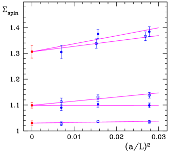
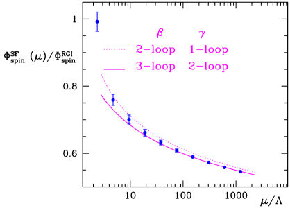
Figure 1: Left: examples of continuum limit extrapolations of $\Sigma_{\rm spin}$ (cf. eqs. (13)) for couplings $u=1.243,2.77\,\mbox{and}\,3.48$. Filled symbols indicate that $F_{\mu\nu}$ was defined as $\hat{F}_{\mu\nu}$ with the link variables replaced by HYP2 [6] links. Right: scale dependence of ${\cal O}_{\mathrm{spin}}$ in the SF scheme with its associated $\Lambda$ parameter [8].

By applying eqs. $(\ref{e:g0b0},\,\ref{e:ZRGIoverZS})$ at weak coupling $\bar{g}^{2}(\mu)$ with the two-loop anomalous dimension in the SF scheme [10, 11],

$$\gamma^{\rm SF}(\bar{g})=-\bar{g}^{2}(\gamma_{0}+\gamma_{1}^{\rm SF}\bar{g}^{2}+\ldots)\,,\quad\gamma_{1}^{\rm SF}=-0.00236-0.00352N_{\rm f}+0.00023N_{\rm f}^{2}\,,$$ (14)

we are able to non-perturbatively connect the low energy regime with the RGI, and arrive at

$$\Phi^{\rm SF}_{\rm spin}(\mu)/\Phi^{\rm RGI}_{\rm spin} = 0.992(29)\,,\qquad\mbox{at $\mu=1/2L_{\rm max}$}\,,\qquad 2L_{\rm max}=1.436r_{0}\,\cite[cite]{[\@@bibref{}{Guagnelli:1998ud}{}{}]}\,.$$ (15)

The latter has to be combined with values of $Z_{\rm spin}^{\rm SF}(2L_{\rm max})$, depending on the bare coupling and lattice action, to form

$$Z_{\rm spin}^{\rm RGI}=Z_{\rm spin}^{\rm SF}(L)\texttimes\Phi^{\rm RGI}_{\rm spin}/\Phi^{\rm SF}_{\rm spin}(1/L)$$ (16)

for the respective action. The numerical values are well represented by

$$Z_{\rm spin}^{\rm SF}(2L_{\rm max})=2.55+0.16(\beta-6)-0.40(\beta-6)^{2}\,,\qquad 6.0\leq\beta\leq 6.5\,,$$ (17)

for the HYP1 [6] action with an error of about 1%. For the other actions see [10].

3 Three-loop matching between HQET and QCD

As pointed out in Sect. 1 the perturbative matching between HQET and QCD plays a very important role in a precise determination of the mass splitting. Our three-loop computation [13] of the matching coefficient and the anomalous dimension of the chromo-magnetic operator allow us to give a reliable final result and estimate its uncertainty.

The coefficient of the chromo-magnetic term needs to be determined by matching to QCD. In perturbation theory we consider the scattering amplitude of an on-shell heavy quark in an external chromo-magnetic field, expanded in the momentum transfer $q$ up to the linear term. Denoting it schematically by ${\cal A}$ and indicating only the presently relevant dependences, we have the (traditional) matching condition (with ${\cal A}_{\mathrm{hqet}}^{\rm\overline{MS\kern-0.35002pt}\kern 0.35002pt}(\mu)=U^{{\rm\overline{MS\kern-0.35002pt}\kern 0.35002pt}}(\mu)\,{\cal A}_{\mathrm{hqet}}^{\mathrm{RGI}}$ as in eq. (9))

$${{\cal A}_{\mathrm{qcd}}}={1\over m_{\rm Q}}\,C_{\rm cm}(m_{\rm Q})U^{{\rm\overline{MS\kern-0.35002pt}\kern 0.35002pt}}(m_{\rm Q})\,{\cal A}_{\mathrm{hqet}}^{\mathrm{RGI}}\,,\quad{\cal A}_{\mathrm{hqet}}^{\mathrm{RGI}}=\langle\beta|{\cal O}_{\mathrm{spin}}^{\rm RGI}|\alpha\rangle\,.$$ (18)

By working in the $\overline{\rm MS}$ scheme and with the background field method [14], we arrive at the 3-loop result for the matching coefficient

$$C_{\rm cm}(m_{\rm Q}) = 1+0.6897\alpha_{{\rm\overline{MS\kern-0.35002pt}\kern 0.35002pt}}(m_{\rm Q})+(2.2182-0.1938N_{\rm f})\alpha_{{\rm\overline{MS\kern-0.35002pt}\kern 0.35002pt}}^{2}(m_{\rm Q})$$

$$+(11.0763-1.7495N_{\rm f}+0.0513N_{\rm f}^{2})\alpha_{{\rm\overline{MS\kern-0.35002pt}\kern 0.35002pt}}^{3}(m_{\rm Q})+{\rm O}(\alpha_{{\rm\overline{MS\kern-0.35002pt}\kern 0.35002pt}}^{4})\,,$$

while for the anomalous dimension of ${\cal O}_{\mathrm{spin}}^{\rm\overline{MS\kern-0.35002pt}\kern 0.35002pt}$, which enters $U^{\rm\overline{MS\kern-0.35002pt}\kern 0.35002pt}(\mu)$, we extract

$$\gamma^{\overline{\rm MS}}(\alpha_{{\rm\overline{MS\kern-0.35002pt}\kern 0.35002pt}}) = 0.4775\alpha_{{\rm\overline{MS\kern-0.35002pt}\kern 0.35002pt}}+(0.4306-0.0549N_{\rm f})\alpha_{{\rm\overline{MS\kern-0.35002pt}\kern 0.35002pt}}^{2}$$

$$+(0.8823-0.1472N_{\rm f}-0.0007N_{\rm f}^{2})\alpha_{{\rm\overline{MS\kern-0.35002pt}\kern 0.35002pt}}^{3}+{\rm O}(\alpha_{{\rm\overline{MS\kern-0.35002pt}\kern 0.35002pt}}^{4})\,.$$

Here, formulae are given for the case where the heavy quarks are quenched also in QCD. Their loop effects are very small [13]. The conversion function $C_{\rm mag}$ of Sect. 1 is obtained by changing the renormalization scheme in the effective theory such as to include the finite renormalization $C_{\rm cm}$, while $C_{\rm spin}$ is constructed by replacing in addition the pole mass, $m_{\rm Q}$, by the RGI mass, $M$:

$${\cal A}_{\mathrm{qcd}}={1\over m_{\rm Q}}\,C_{\rm mag}(M/\Lambda_{\rm\overline{MS\kern-0.35002pt}\kern 0.35002pt})\,{\cal A}_{\mathrm{hqet}}^{\mathrm{RGI}}={1\over M}\,C_{\rm spin}(M/\Lambda_{\rm\overline{MS\kern-0.35002pt}\kern 0.35002pt})\,{\cal A}_{\mathrm{hqet}}^{\mathrm{RGI}}\,.$$ (21)

The resulting equations

$$C_{\rm spin}(M/\Lambda_{\rm\overline{MS\kern-0.35002pt}\kern 0.35002pt})\equiv U^{\mathrm{spin}}(\kern 1.0pt\overline{\kern-1.0ptm\kern-1.0pt}\kern 1.0pt_{*})={M\over m_{\rm Q}}C_{\rm mag}(M/\Lambda_{\rm\overline{MS\kern-0.35002pt}\kern 0.35002pt})\equiv{M\over m_{\rm Q}}U^{\mathrm{mag}}(\kern 1.0pt\overline{\kern-1.0ptm\kern-1.0pt}\kern 1.0pt_{*})$$ (22)

then define the anomalous dimensions $\gamma^{\mathrm{spin}}\,,\,\gamma^{\mathrm{mag}}$. In all these schemes the renormalization of the coupling remains untouched: ${\rm\overline{MS\kern-0.50003pt}\kern 0.50003pt}$. The change from the ${\rm\overline{MS\kern-0.50003pt}\kern 0.50003pt}$-mass at its own scale $\kern 1.0pt\overline{\kern-1.0ptm\kern-1.0pt}\kern 1.0pt_{*}$ as argument of $U^{\mathrm{spin}}$ to the RGI-mass as the argument of $C_{\rm spin}$ is convenient since the RGI-masses are the primary quantities obtained in a non-perturbative lattice computation [4].

The second equation in (21) avoids the pole mass which is known to have a bad perturbative expansion in terms of short distance masses (or $M$). Thus the anomalous dimension $\gamma^{\mathrm{spin}}$ is expected to show a better behaved perturbative series which will be reflected in $C_{\rm spin}$.

For practical purposes we parametrize the conversion functions $C_{\rm spin}$ and $C_{\rm mag}$ in the $N_{\rm f}=0$ theory, graphically represented in Figure 2, in terms of the variable $x\equiv 1/\ln(M/\Lambda_{\rm\overline{MS\kern-0.35002pt}\kern 0.35002pt})$:

$$C_{\rm spin}=\left\{\begin{array}[]{ll}x^{\gamma_{0}^{\rm spin}/(2b_{0})}\{1+0.087x-0.021x^{2}\}&\mbox{2-loop $\gamma$}\\ x^{\gamma_{0}^{\rm spin}/(2b_{0})}\{1+0.097x+0.115x^{2}-0.038x^{3}\}&\mbox{3-loop $\gamma$}\\ \end{array}\right.\,,\quad\gamma_{0}^{\rm spin}=-2/(4\pi)^{2}\,.$$ (23)

These formulae guarantee at least 0.3% precision for $x\leq 0.6$. Inspection of Figure 2 shows the expected bad perturbative behavior of $C_{\rm mag}$. We thus focus our attention on $C_{\rm spin}$ which exhibits very small higher order contributions in the b-region. The difference $\Delta C_{\rm spin}(M_{\rm b}/\Lambda)\approx 10^{-2}$ between the three-loop and the two-loop determination with $M_{\rm b}=6.76(9)\,{\rm GeV}$ (from [15]) is much smaller than the statistical error on the spin splitting presented in the following section. Evaluating it with an estimate (where the four-loop term in the very well behaved $\gamma^{\rm\overline{MS\kern-0.35002pt}\kern 0.35002pt}$ is neglected) for the anomalous dimension $\gamma^{\mathrm{spin}}$ gives $\Delta C_{\rm spin}(M_{\rm b}/\Lambda)\approx 10^{-2}$ with respect to the three-loop estimate. We thus claim an about 1% relative error for $C_{\rm spin}$ evaluated with the three-loop $\gamma^{\mathrm{spin}}$ for B-physics applications. For $N_{\rm f}=4$ the behavior of $C_{\rm mag}$ and $C_{\rm spin}$ is very similar to Fig. 2 [13].

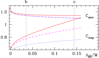
Figure 2: Conversion functions for $N_{\rm f}=0$. Dotted, dashed and solid lines use the one-, two- and three-loop anomalous dimension. The abscissae of the b- and c-quark [15, 11, 16, 17] are marked by dotted lines.

4 First results for the spin-splitting and outlook

As a first application we take quenched results for the bare $\lambda_{2}$ from the literature and exploit our results (16, 23). Unfortunately they exist only for $\beta=6.0$, corresponding to $a\approx 0.1$ fm,

$$\mbox{Ref.}~{}\cite[cite]{[\@@bibref{}{Gimenez:1996av}{}{}]}:\quad\Delta m^{2}=0.28(6)(?)\,{\rm GeV}^{2}\,\,\stackrel{{\scriptstyle(\ref{e:ZspinRGI},\,\ref{e:Cspin_para})}}{{\longrightarrow}}\,\,\Delta m^{2}=0.38(7)(?)\,{\rm GeV}^{2}\,,$$ (24)

$$\mbox{Ref.}~{}\cite[cite]{[\@@bibref{}{Aoki:2003jf}{}{}]}:\quad\Delta m^{2}=0.36(4)(?)\,{\rm GeV}^{2}\,\,\stackrel{{\scriptstyle(\ref{e:ZspinRGI},\,\ref{e:Cspin_para})}}{{\longrightarrow}}\,\,\Delta m^{2}=0.53(6)(?)\,{\rm GeV}^{2}\,,$$ (25)

where the numbers on the l.h.s. are taken from the corresponding references, performing a perturbative renormalization. On the r.h.s. we used the b-quark mass from [15] and the 3-loop determination of $C_{\rm spin}$. The uncertainty marked as $(?)$ refers to lattice artefacts and the missing dynamical quark determinant. The central values are now closer to the experimental mass splitting, $\Delta m^{2}=0.497\,{\rm GeV}^{2}$, but at the moment the large uncertainties prevent us from concluding that indeed the quenched approximation can give a good estimate of this observable.

As explained in [10], the same renormalization factor applies to spin-dependent potentials [20, 21], where so far only a perturbative renormalization was possible.

The non-perturbative computation of $Z_{\rm spin}^{\rm RGI}$ has demonstrated the applicability of the Schrödinger functional renormalization programme [22, 23] to another difficult case. Quite significant deviations from the perturbative scale evolution are present at low energies, see Figure 1.

With respect to a perturbative estimate, the new $Z_{\rm spin}^{\rm RGI}$ has a rather big effect. Furthermore, thanks to the results presented in Sect. 3, which extend [24, 25, 26, 27, 28], we can match the effective theory and QCD introducing an error in practice negligible in comparison to all other uncertainties entering $\Delta m^{2}$. It now remains to compute $\lambda_{2}^{\rm bare}$ with higher precision and perform the continuum limit. However, due to the large amount of statistics needed especially at large couplings, an extension of this method to the dynamical quarks case seems difficult. In this direction, other, fully non-perturbative, approaches are more promising at present [16, 11, 29, 15].

Acknowledgements. We thank M. Della Morte, J. Flynn, B. Leder, S. Takeda and U. Wolff for fruitful discussions. This work is supported by the Deutsche Forschungsgemeinschaft in the SFB/TR 09, by the European community through EU Contract No. MRTN-CT-2006-035482, “FLAVIAnet” and by funds provided by the U.S. Department of Energy under cooperative research agreement DE-FC02-94ER40818.

References

- [1] E. Eichten and B.R. Hill, Phys. Lett. B234 (1990) 511.
- [2] B. Grinstein, Nucl. Phys. B339 (1990) 253.
- [3] H. Georgi, Phys. Lett. B240 (1990) 447.
- [4] ALPHA, S. Capitani, M. Lüscher, R. Sommer and H. Wittig, Nucl. Phys. B544 (1999) 669, hep-lat/9810063.
- [5] R. Sommer, (2006), hep-lat/0611020.
- [6] M. Della Morte, A. Shindler and R. Sommer, JHEP 08 (2005) 051, hep-lat/0506008.
- [7] ALPHA, M. Kurth and R. Sommer, Nucl. Phys. B597 (2001) 488, hep-lat/0007002.
- [8] M. Lüscher, R. Sommer, P. Weisz and U. Wolff, Nucl. Phys. B413 (1994) 481, hep-lat/9309005.
- [9] M. Lüscher, S. Sint, R. Sommer and P. Weisz, Nucl. Phys. B478 (1996) 365, hep-lat/9605038.
- [10] ALPHA, D. Guazzini, H.B. Meyer and R. Sommer, (2007), arXiv:0705.1809 [hep-lat], accepted for publication in JHEP.
- [11] D. Guazzini, Heavy-light mesons in lattice HQET and QCD, PhD thesis, Humboldt Universität zu Berlin and DESY Zeuthen, Berlin and Zeuthen, Germany, 2007.
- [12] ALPHA, M. Guagnelli, R. Sommer and H. Wittig, Nucl. Phys. B535 (1998) 389, hep-lat/9806005.
- [13] A.G. Grozin, P. Marquard, J.H. Piclum and M. Steinhauser, (2007), arXiv:0707.1388 [hep-ph], accepted for publication in Nucl. Phys. B.
- [14] L.F. Abbott, Nucl. Phys. B185 (1981) 189.
- [15] M. Della Morte, N. Garron, M. Papinutto and R. Sommer, JHEP 01 (2007) 007, hep-ph/0609294.
- [16] D. Guazzini, R. Sommer and N. Tantalo, PoS LAT2006 (2006) 084, hep-lat/0609065.
- [17] ALPHA, J. Rolf and S. Sint, JHEP 12 (2002) 007, hep-ph/0209255.
- [18] V. Gimenez, G. Martinelli and C.T. Sachrajda, Nucl. Phys. B486 (1997) 227, hep-lat/9607055.
- [19] JLQCD, S. Aoki et al., Phys. Rev. D69 (2004) 094512, hep-lat/0305024.
- [20] E. Eichten and F. Feinberg, Phys. Rev. D23 (1981) 2724.
- [21] A. Vairo, (2007), arXiv:0709.3341 [hep-ph].
- [22] M. Lüscher, P. Weisz and U. Wolff, Nucl. Phys. B359 (1991) 221.
- [23] ALPHA, A. Bode et al., Phys. Lett. B515 (2001) 49, hep-lat/0105003.
- [24] E. Eichten and B.R. Hill, Phys. Lett. B243 (1990) 427.
- [25] A.F. Falk, B. Grinstein and M.E. Luke, Nucl. Phys. B357 (1991) 185.
- [26] G. Amoros, M. Beneke and M. Neubert, Phys. Lett. B401 (1997) 81, hep-ph/9701375.
- [27] A. Czarnecki and A.G. Grozin, Phys. Lett. B405 (1997) 142, hep-ph/9701415.
- [28] ALPHA, J. Heitger, A. Jüttner, R. Sommer and J. Wennekers, JHEP 11 (2004) 048, hep-ph/0407227.
- [29] ALPHA, J. Heitger and R. Sommer, JHEP 02 (2004) 022, hep-lat/0310035.