Long time limit of equilibrium glassy dynamics and replica calculation

Abstract

It is shown that the limit $t-t^{\prime}\to\infty$ of the equilibrium dynamic self-energy can be computed from the $n\to 1$ limit of the static self-energy of a $n$-times replicated system with one step replica symmetry breaking structure. It is also shown that the Dyson equation of the replicated system leads in the $n\to 1$ limit to the bifurcation equation for the glass ergodicity breaking parameter computed from dynamics. The equivalence of the replica formalism to the long time limit of the equilibrium relaxation dynamics is proved to all orders in perturbation for a scalar theory.

I Introduction

Spin glass and structural glasses are characterized by the presence of a complex structure of stable and metastable states metastable . The basic idea KirThi87 ; CriSom92 ; CriHorSom93 ; BouMez94 ; MarParRit94 ; CriSom95 ; BouCugKurMez96 , supported by the behavior of some mean-field spin glass models, is that the glassy behavior arises because of the emergence of an exponentially large number of metastable states that breaks the ergodicity and prevents the system from reaching the true thermodynamic equilibrium state. The logarithm of the number of metastable state is commonly called “complexity” or “configurational” entropy. The glass transition is then associated with the emergence of a non-zero configurational entropy. By extending the replica method, originally developed for disordered systems, the occurrence of a non-zero configurational entropy can be conveniently studied within the replica formalism Monasson95 .

The basic idea of the replica approach Monasson95 ; MezPar99 ; ColMezParVer99 ; MezPar00 ; ParZam05 ; ParZam06 is to consider the equilibrium a thermodynamics of $m$ copies of the original system interacting among them via an infinitesimal attractive coupling. If the free-energy landscape breaks down into (exponentially) many metastable states, the $m$ copies will then condensate into the same metastable state since their relative distances in such states are smaller than in the liquid (paramagnetic) phase. The replica method allow for an equilibrium analysis of the properties of the metastable states, in spite of the fact that these are originally defined in a dynamic framework. In particular the properties of the original system is recovered continuing the replica number $m$ to $m\leq 1$ and taking in the limit $m\to 1$.

If one applies the present method to mean-field $p$-spin spin glass models, whose low temperature phase is described by a one replica symmetry breaking step (1RSB), the result agrees with that from a dynamical study. We observe that in this case the number $m$ of replicas corresponds to the break point of the 1RSB solution of the conventional replica approach, and hence the $m\to 1$ limit clearly corresponds to the onset of the glass phase.

All checks of the equivalence between the replica approach and the dynamical approach we are aware of GroKraTarVio02 ; WesSchWol03 ; MiyRei05 ; AndBirLef06 , use some approximations to compute the relevant correlation functions of the many-body problem. These leave open the possibility that the equivalence is just a consequence of the limited number of dynamical diagrams considered in the various approximations.

To our knowledge the equivalence of two approaches for a general system is not yet proved. The proof of this statement is the main result reported in this paper. To be more specific, in this paper we show under rather general assumptions, that the long time limit $t-t^{\prime}\to\infty$ of the equilibrium two-times correlation function of a glassy system can be computed from the $n\to 1$ limit of the static theory of an $n$-times replicated system with a 1RSB structure. The proof is based, following similar works Naketal83 ; Gozzi83 on the connection between static and equilibrium dynamics, on a suitable summation of classes of dynamical diagrams of the dynamic perturbation theory generated by the Langevin dynamics, and showing that in the limit $t-t^{\prime}\to\infty$ these approaches those of the $n\to 1$ limit of the equilibrium theory of an $n$-times replicated system with a 1RSB structure.

The reader will not find in this paper the physical consequences that can be obtained for specific systems or models by using the results reported here. For these the interested reader is referred to, e.g., Ref. [GroKraTarVio02, ; WesSchWol03, ; MiyRei05, ; AndBirLef06, ] or to the forthcoming paper BirCriprep where these will be applied to a simple toy system.

To keep the notation as simple as possible we shall consider only scalar fields. The generalization to more complex fields, e.g., vector field, is straightforward. Our starting point is hence the Langevin equation of the form

$$\frac{\partial\varphi(t)}{\partial t}=-\frac{\delta H[\varphi]}{\delta\varphi(t)}+\eta(t)$$ (1)

which describes the purely relaxation dynamics towards equilibrium of the scalar stochastic field $\varphi$ in presence of the stochastic force $\eta$. In general both $\varphi$ and $\eta$ can be functions of both time and space coordinates however, since we are interested into the time behavior of correlations, space coordinates can be safely neglected. As a consequence we shall drop any explicit space dependence of fields. The Hamiltonian $H[\varphi]$ governs the behavior of the system. Here, when needed to illustrate the calculations, we shall use

$$H[\varphi]=\frac{r}{2}\,\varphi^{2}+\frac{\lambda}{4!}\,\varphi^{4}$$ (2)

which describes a zero-dimensional scalar $\varphi^{4}$ theory.

The stochastic force $\eta$ has a Gaussian distribution of zero mean and second moment fixed by the Einstein’s relation

$$\langle\eta(t)\,\eta(t^{\prime})\rangle=2T\,\delta(t-t^{\prime})$$ (3)

where $T$ is the temperature. Indeed, as can be verified by means of the associated Fokker-Planck equation risken , eq. (3) guarantees that the time dependent probability distribution function $P[\varphi,t]$ eventually converge for $t\to\infty$ to the equilibrium distribution

$$P_{\rm eq}[\varphi]\propto\exp(-\beta\,H[\varphi]),$$ (4)

where $\beta=T^{-1}$.

Given an initial condition $\varphi(t_{0})$ the expectation value of a generic observable ${\cal O}[\varphi]$ over the stochastic process generated by the Langevin equation (1) can be written as the path integral MarSigRos73 ; DeDom75 ; DeDom76 ; Janssen76 ; BauJanWag76 ; DeDomPel78

$$\langle{\cal O}\rangle=\int\,{\cal D}\varphi\,{\cal D}\hat{\varphi}\ {\cal O}[\varphi]\,{\rm e}^{-S[\varphi,\hat{\varphi}]}$$ (5)

where

$$S[\varphi,\hat{\varphi}]=\int_{t_{0}}^{\infty}\,dt\ \left\{\hat{\varphi}\left[\partial_{t}\varphi+\frac{\delta H[\varphi]}{\delta\varphi(t)}\right]-\hat{\varphi}\,T\,\hat{\varphi}\right\}$$ (6)

The dynamical functional $S[\varphi,\hat{\varphi}]$ takes the form of a statistical field theory with two independent sets of fields, the original field $\varphi$ and the response field $\hat{\varphi}$, so that all well established machinery of statistical and quantum field theory can be applied. The field $\hat{\varphi}$ is called “response field” since it is conjugated to an external field $h$. As a consequence arbitrary response functions can be generated by taking correlators involving $\hat{\varphi}$-fields. In particular the dynamic susceptibility or response function $G(t,s)$ reads

$$G(t,s)=\left.\frac{\delta\langle\varphi(t)\rangle}{\delta h(s)}\right|_{h=0}=\beta\,\langle\varphi(t)\,\hat{\varphi}(s)\rangle,\qquad t>s.$$ (7)

From now on we absorb the factor $\beta$ into the definition of the response function.

We note that in deriving the dynamical functional $S[\varphi,\hat{\varphi}]$ we have assumed the Ito prescription for the stochastic calculus. This implies that $G(t,t)=0$. Accordingly, in a perturbative expansion of averages (5) all diagrams with at least one loop of the response function can be neglected.

In equilibrium the response function $G(t,s)$ is related to the two point correlation function $C(t,s)=\langle\varphi(t)\,\varphi(s)\rangle$ by the fluctuation-dissipation theorem (FDT):

$$G(t,s)=\theta(t-s)\frac{\partial}{\partial s}\,C(t,s)=-\theta(t-s)\frac{\partial}{\partial t}\,C(t,s)$$ (8)

We note that time translation invariance of equilibrium implies that all two-points correlators are function of the time difference only. This functional dependence is always assumed, even if not explicitly shown, every times we consider equilibrium correlators.

In equilibrium the calculation of the two point correlation function $C(t,t^{\prime})$ can be reduced to that of the dynamic self-energy $\Sigma_{\hat{\varphi}\hat{\varphi}}(t,t^{\prime})$. Indeed by using standard methods of statistical field theory zinn and the FDT relation (8) one obtains for $C(t,t^{\prime})$ the following equation, valid for $t>t^{\prime}$:

$$\bigl{[}\partial_{t}+H^{\prime\prime}[0]-\Sigma_{\hat{\varphi}\hat{\varphi}}(t,t)\bigr{]}\,C(t,t^{\prime})+\int_{t^{\prime}}^{t}\,ds\,\Sigma_{\hat{\varphi}\hat{\varphi}}(t,s)\,\partial_{s}C(s,t^{\prime})=0\qquad t>t^{\prime}$$ (9)

where

$$H^{\prime\prime}[0]\equiv\left.\frac{\delta^{2}H[\varphi]}{\delta\varphi^{2}}\right|_{\varphi=0}$$ (10)

is the quadratic part of the Hamiltonian $H[\varphi]$. For simplicity we assume that in equilibrium $\langle\varphi\rangle=0$.

In glassy systems the correlation function $C(t,t^{\prime})$ does not vanish in long-time limit $t-t^{\prime}\to\infty$:

$$\lim_{t-t^{\prime}\to\infty}C(t,t^{\prime})=C(\infty)\not=0$$ (11)

signaling the breaking of the ergodicity gotze . The value of the “ergodicity breaking parameter” $C(\infty)$ is obtained by taking $t-t^{\prime}\to\infty$ limit of eq. (9):

$$\bigl{[}H^{\prime\prime}[0]-\Sigma_{\hat{\varphi}\hat{\varphi}}(0)\bigr{]}\,C(\infty)+\bigl{[}C(\infty)-C(0)\bigr{]}\,\Sigma_{\hat{\varphi}\hat{\varphi}}(\infty)=0$$ (12)

where $\Sigma_{\hat{\varphi}\hat{\varphi}}(\infty)$ is the $t-t^{\prime}\to\infty$ limit of $\Sigma_{\hat{\varphi}\hat{\varphi}}(t,t^{\prime})$, while $C(0)=C(t,t)$ and $\Sigma_{\hat{\varphi}\hat{\varphi}}(0)=\Sigma_{\hat{\varphi}\hat{\varphi}}(t,t)$ are the equal-time value of the correlation and self-energy. The latter can be eliminated using the relation

$$\bigl{[}H^{\prime\prime}[0]-\Sigma_{\hat{\varphi}\hat{\varphi}}(0)\bigr{]}\,C(0)=1$$ (13)

that follows form the $t\to t^{\prime+}$ limit of equation (9) and $\lim_{t\to t^{\prime+}}\partial_{t}C(t,t^{\prime})=-1$. By combining together eq. (12) and eq. (13) we finally obtain the bifurcation equation

$$\frac{C(\infty)}{C(0)}-C(0)\,\Sigma_{\hat{\varphi}\hat{\varphi}}(\infty)\left[1-\frac{C(\infty)}{C(0)}\right]=0.$$ (14)

In this approach the glass transition is signaled by the appearance of a non-trivial solution of the bifurcation equation.

The calculation of the dynamic self-energy $\Sigma_{\hat{\varphi}\hat{\varphi}}(t,t^{\prime})$ is in general a non trivial task and approximations are usually required to deal with the diagrams of the dynamical perturbation theory. In this paper we shall show that in the limit of $t-t^{\prime}\to\infty$ the calculation of the dynamic diagrams simplifies and the bifurcation equation (14) can be obtained from a purely static calculation of a $n$-times replicated system with a 1RSB structure.

The paper is organized as follows. In Section II we shall study the structure of the equilibrium diagrammatic expansion of the dynamic self-energy $\Sigma_{\hat{\varphi}\hat{\varphi}}(t,t^{\prime})$. We shall show that for $t>t^{\prime}$ $\Sigma_{\hat{\varphi}\hat{\varphi}}(t,t^{\prime})$ can be decomposed into the sum of classes of diagrams obtained by a suitable rearrangement and partial summation of dynamical diagrams. In Section III we shall consider the limit $t-t^{\prime}\to\infty$ of the self-energy $\Sigma_{\hat{\varphi}\hat{\varphi}}(t,t^{\prime})$. Here, using both a sum rule approach and a diagrammatic approach, we shall prove that in the limit $t-t^{\prime}\to\infty$ all time integrals of the diagrammatic expansion can be evaluated and that the self-energy $\Sigma_{\hat{\varphi}\hat{\varphi}}(\infty)$ is a function of $C(0)$ and $C(\infty)$ only. In Section IV we develop the replica calculation. We shall show that $\Sigma_{\hat{\varphi}\hat{\varphi}}(\infty)$ evaluated in Section III is equal to the static self-energy of an $n$-times replicated system with a 1RSB structure when the limit $n\to 1$ is taken. This result allows us to derive the bifurcation equation (14) on a purely static calculation.

II Equilibrium Dynamic Self-Energy: $t-t^{\prime}$ finite

The self-energy gives the correction to the free theory correlators when interactions are taken into account. Its calculation is in general rather difficult and one is obliged to use some approximation schemes. Following standard field theory procedures zinn ; lebellac a systematic perturbative calculation of the self-energy can be established in terms of the so called proper vertex functions. Diagrammatically these quantities are represented by the sets of one-particle irreducible (1PI) diagrams, i.e., by diagrams that do not split into two subdiagrams by cutting any single propagator line, with all the external incoming $\varphi$ and outgoing $\hat{\varphi}$ legs amputated.

II.1 Equilibrium Dynamic Diagrams

The self-energy $\Sigma_{\hat{\varphi}\hat{\varphi}}(t,t^{\prime})$ is related to the proper vertex with the two external outgoing $\hat{\varphi}$ legs removed. The equilibrium diagrammatic expansion of the dynamic self-energy $\Sigma_{\hat{\varphi}\hat{\varphi}}(t,t^{\prime})$ takes then the following form

$$\Sigma_{\hat{\varphi}\hat{\varphi}}(t,t^{\prime})=\ \includegraphics[scale={1.0},bb=152 603 325 634]{sigma_exp.eps}$$ (15)

where each line connecting the two vertices represents the full correlation function DeDom63 ; CorJacTom74 ; Haymaker91

$$C(s,s^{\prime})\equiv\langle\varphi(s)\,\varphi(s^{\prime})\rangle=\ \includegraphics[bb=201 620 263 644]{corr.eps}$$ (16)

The full (left) vertex with $1+r$ external legs is the sum of all connected 1PI dynamic diagrams with the outgoing $\hat{\varphi}$ leg at $t$, the wiggly line in (15), and $r$ incoming $\varphi$ legs at times $s_{1},\ldots,s_{r}$ ($\leq t$) removed. To each internal $\varphi\varphi$-line connecting the internal vertices at times $s^{\prime}$ and $s$ is associated the full correlation function $C(s,s^{\prime})$ while to each internal $\varphi\hat{\varphi}$-line connecting the internal vertices at times $s^{\prime}$ and $s$ is associated the full response function DeDom63 ; CorJacTom74 ; Haymaker91

$$G(s,s^{\prime})\equiv\langle\varphi(s)\,\hat{\varphi}(s^{\prime})\rangle=\ \includegraphics[bb=201 620 263 644]{resp.eps}$$ (17)

with $s>s^{\prime}$. All internal times are integrated from $t^{\prime}$ to $t$.

The empty (right) vertex with $1+r$ external legs is built from the same 1PI diagrams of the full vertex but with all external times times $t,s_{1}\ldots,s_{r}$ equal to $t^{\prime}$. As a consequence, since in equilibrium the correlation and response functions are related by FDT, it is given by the topological equivalent vertex obtained from the associated static equilibrium theory described by the canonical distribution (4) Naketal83 .

The structure just described can be understood as follows. First of all we note that since closed loops of response function vanish, each internal vertex of the 1PI diagrams contributing to the self-energy $\Sigma_{\hat{\varphi}\hat{\varphi}}(t,t^{\prime})$ is connected via $\varphi\hat{\varphi}$-lines to one or the other of the external wiggly lines, but not to both. This means that the diagram can be divided into two subdiagrams made of all the vertices connected to the same external wiggly line. The two subdiagrams are clearly 1PI and joined together by $2$ or more $\varphi\varphi$-lines. It is easy to recognize the two subdiagrams as the full/empty vertices.

Alternatively one can invoke the general diagrammatic expansion of the correlation function $\langle\varphi(t)\,\varphi(t^{\prime})\rangle$ as the matching of two tree expansions ma , one for $\varphi(t)$ and one for $\varphi(t^{\prime})$, and note that the lines connecting the full/empty vertices are the lines joining the two tree expansions. We note that the assumption that the system is at equilibrium implies that all two-times quantities depend only on time difference. Then the contribution from the tree expansion of $\varphi(t^{\prime})$ averaged over noise and equilibrium initial conditions, the empty vertices, cannot depend on time $t^{\prime}$ and must be equal to that obtained from the equilibrium static theory described by the canonical distribution (4) with all lines equal to the static equilibrium correlation function $C(t^{\prime},t^{\prime})\equiv C(0)$.

The internal structure of the empty vertices can be inferred by using the following dynamical functional, see Appendix C,

$$S^{\prime}[\varphi,\hat{\varphi}]=S[\varphi,\hat{\varphi}]+\int_{t_{0}}^{\infty}\,ds\,H[\varphi(s)]\,\delta(s-t_{0})$$ (18)

to impose statistical equilibrium with the canonical distribution (4) at the initial time $t_{0}$ . The analysis of the dynamic diagrams generated by $S^{\prime}[\varphi,\hat{\varphi}]$ shows that the effect of the last term is that of canceling out from all dynamic diagrams for $\Sigma_{\hat{\varphi}\hat{\varphi}}(t,t^{\prime})$ the contribution from times $t_{0}<s<t^{\prime}$ yielding for $\Sigma_{\hat{\varphi}\hat{\varphi}}(t,t^{\prime})$ the equilibrium dynamic diagrammatic expansion discussed above. This can be understood on a general ground as follows. The canonical distribution (4) is a stationary solution of the associated Fokker-Planck equation, and hence the probability distribution of $\varphi$ remains canonical for any time past $t_{0}$. Consequence of this is that all quantities evaluated from $S^{\prime}[\varphi,\hat{\varphi}]$ cannot depend on $t_{0}$. This guarantees, for example, that all two-times quantities depend only on time differences. In evaluating $\Sigma_{\hat{\varphi}\hat{\varphi}}(t,t^{\prime})$ for $t>t^{\prime}$ we can then choose for $t_{0}$ in (18) any value $\leq t^{\prime}$. The invariance property ensures that we always get the same diagrams. Clearly the simplest choice is $t_{0}=t^{\prime}$ which, in turn, implies that in the diagrammatic dynamical perturbative expansion all free times must be integrated from $t^{\prime}$. We have seen that the dynamical diagrams for $\Sigma_{\hat{\varphi}\hat{\varphi}}(t,t^{\prime})$ generated by $S[\varphi,\hat{\varphi}]$ can be divided into two subdiagrams, joined by $r\geq 2$ correlation lines, by grouping together all vertices connected by response $\varphi\hat{\varphi}$-lines to the same external (amputated) wiggly line at $t$ or $t^{\prime}$, respectively. The dynamical diagrams generated by $S^{\prime}[\varphi,\hat{\varphi}]$ can be divided in a similar way into two subdiagrams connected by $r$ correlation lines just grouping together all vertices connected by response $\varphi\hat{\varphi}$-lines to the external (amputated) wiggly line at $t$. It is easy to realize that this procedure leads to the same full vertex obtained from $S[\varphi,\hat{\varphi}]$, while the (putative) empty vertex, the one connected to external (amputated) leg at $t^{\prime}$, contains now only contributions from the last term in (18) since the equal time response function vanishes. Stated in a different way, the empty vertex contains only the diagrams generated by the equilibrium initial condition, i.e., it is equal to topological equivalent 1PI diagram with $1+r$ external (amputated) legs of the associated static theory described by the canonical distribution (4) with all $\varphi\varphi$-lines equal to the static equilibrium correlation function $C(t,t)\equiv C(0)$. The same conclusion can be obtained by first dividing the dynamical diagrams generated by $S^{\prime}[\varphi,\hat{\varphi}]$ as described above, and then taking the limit $t_{0}\to t^{\prime}$ directly on diagrams.

The definition of empty vertex given above uses $S[\varphi,\hat{\varphi}]$ and follows from the observation that the equilibrium FDT relation between response and correlation function guarantees that setting all external times of a dynamic diagram equal to each other reduces the dynamic diagram to the topological equivalent diagram of the associated static equilibrium theory Naketal83 .

We can then summarize the rules for writing down the equilibrium dynamic diagrams for $\Sigma_{\hat{\varphi}\hat{\varphi}}(t,t^{\prime})$:

1. Write down the dynamic diagrams generated by the dynamical functional $S[\varphi,\hat{\varphi}]$ using the standard dynamical rules, neglecting all numerical symmetry factors.

2. In each diagram remove the minimal number of $C$-lines needed to divide the diagram into two disjoint sub-diagrams so that in the first (left) sub-diagram all vertices are connected to time $t$ through $G$-lines, while in the second (right) sub-diagram are connected through $G$-lines to time $t^{\prime}$.

3. In the second (right) sub-diagram, the one connected to $t^{\prime}$, replace all response $G$-lines by correlation $C$-lines, and set all time variables to $t^{\prime}$.

4. If after replacement two or more different dynamic diagrams lead to the same diagram count the latter only once.

5. Multiply each diagram so obtained by the appropriate numerical symmetry factor and evaluate it with the usual rules integrating all left internal times from $t^{\prime}$ to $t$.

To illustrate the above rules consider the third order dynamic diagrams shown in Fig. 1 generated by the dynamical functional $S^{\prime}[\varphi,\hat{\varphi}]$ (18) for the scalar zero-dimensional $\varphi^{4}$ theory (2).

Figure 1: Third order dynamic diagrams with equilibrium condition at $t_{0}$.

By using the standard dynamic rules the contribution of these diagrams is

$$\Sigma_{\hat{\varphi}\hat{\varphi}}^{(3)}(t,t^{\prime}) = \frac{1}{2}\int_{t_{0}}^{t}ds\,G(t,s)\,C(t,s)\,C^{2}(t^{\prime},s)\,C(t,t^{\prime})+\frac{1}{2}\int_{t_{0}}^{t^{\prime}}ds\,C^{2}(t,s)\,G(t^{\prime},s)\,C(t^{\prime},s)\,C(t,t^{\prime})$$ (19)

$$+\frac{1}{4}C^{2}(t,t_{0})\,C^{2}(t^{\prime},t_{0})\,C(t,t^{\prime})$$

With the help of the FDT relation (8) the contribution can be rewritten as

$$\Sigma_{\hat{\varphi}\hat{\varphi}}^{(3)}(t,t^{\prime}) = \frac{1}{4}\int_{t^{\prime}}^{t}ds\,\partial_{s}C^{2}(t,s)\,C^{2}(t^{\prime},s)\,C(t,t^{\prime})+\frac{1}{4}\int_{t_{0}}^{t^{\prime}}ds\,\partial_{s}[C^{2}(t,s)\,C^{2}(t^{\prime},s)]\,C(t,t^{\prime})$$ (20)

$$+\frac{1}{4}C^{2}(t,t_{0})\,C^{2}(t^{\prime},t_{0})\,C(t,t^{\prime})$$

$$= \frac{1}{2}\int_{t^{\prime}}^{t}ds\,G(t,s)\,C(t,s)\,C^{2}(s,t^{\prime})\,C(t,t^{\prime})+\frac{1}{4}C^{3}(t,t^{\prime})\,C^{2}(t^{\prime},t^{\prime})$$

The relevant third order diagrams for the equilibrium dynamic rules, point 1), are the first two diagram in Fig. 1. The decomposition of points 2)-4) leads to the equilibrium diagrams shown in Fig. 2. The two diagrams are easily evaluated and one recovers the result (20).

Figure 2: Third order equilibrium dynamic diagrams.

II.2 Self-Energy Base Diagrams

By reversing the rules to write down the equilibrium dynamic diagrams it follows that each equilibrium dynamic diagram can be obtained by a suitable decoration of a base diagram, i.e., of the diagram with the same topology of the equilibrium dynamic diagram. For example the base diagram for the dynamic diagrams of the previous example is the one shown in Fig. 3.

Figure 3: Third order base diagram.

The equilibrium dynamic diagram is generated from the base diagram by:

1. dividing the base diagram into two sub-diagrams by cutting some lines to reproduce the topology of point 2) of the equilibrium dynamic rules.

2. In the (left) sub-diagram associated to the full vertex attach a $\hat{\varphi}$-line to each vertex to generate the desired $G$-line connection structure.

It is clear that the base diagram is by construction the dynamic diagram in which all $G$-lines are replaced by $C$-lines. As a consequence the self-energy base diagrams are the static self-energy diagrams of the associated equilibrium static theory described by the canonical distribution (4).

II.3 Partial summation of full vertex diagrams

From the structure (15) of the diagrammatic expansion of the self-energy it is easy to realize that also each dynamic diagram contributing to the full vertex with $1+r$ external legs can be obtained from a suitable (static) base diagram by attaching to each internal vertices one $\hat{\varphi}$-line to generate the desired $G$-line structure. Figure 4 shows a base diagram for the $1+3$ full vertex and the three different dynamic diagrams that can be generated.

Figure 4: A base diagram for the $1+3$ full vertex and the three different dynamic diagrams that can be generated. The numerical symmetry factors are not displayed.

A convenient way of imposing that to each vertex is attached one and only one $G$-line is by means of anti-commuting Grassman variables. Following Ref. [Naketal83, ] we then introduce for each vertex the pair of conjugated Grassman variables $(\alpha_{s},\overline{\alpha}_{s})$, where $s$ is the time variable label of the vertex. By using the FDT relation (8) and the properties of Grassman variables it is easy to see that

$$C[s-s^{\prime}+\overline{\alpha}_{s}\alpha_{s}\theta(s^{\prime}-s)-\overline{\alpha}_{s^{\prime}}\alpha_{s^{\prime}}\theta(s-s^{\prime})]$$ (21)

$$\hskip-85.35826pt=C(s-s^{\prime})+\overline{\alpha}_{s}\alpha_{s}\theta(s^{\prime}-s)\partial_{s^{\prime}-s}C(s-s^{\prime})+\overline{\alpha}_{s^{\prime}}\alpha_{s^{\prime}}\theta(s-s^{\prime})\partial_{s^{\prime}-s}C(s-s^{\prime})$$

$$\hskip-85.35826pt=C(s^{\prime},s)+\overline{\alpha}_{s}\alpha_{s}G(s^{\prime},s)+\overline{\alpha}_{s^{\prime}}\alpha_{s^{\prime}}G(s,s^{\prime}).$$

The last equality follows from even parity of the correlation function $C(t,s)=C(s,t)$. Equation (21) has the following simple diagrammatic representation:

$$C[s-s^{\prime}+\overline{\alpha}_{s}\alpha_{s}\theta(s^{\prime}-s)-\overline{\alpha}_{s^{\prime}}\alpha_{s^{\prime}}\theta(s-s^{\prime})]=\includegraphics[scale={0.8},bb=201 620 263 644]{corr.eps}+\overline{\alpha}_{s}\alpha_{s}\includegraphics[scale={0.8},bb=201 620 263 644]{resp-back.eps}+\overline{\alpha}_{s^{\prime}}\alpha_{s^{\prime}}\includegraphics[scale={0.8},bb=201 620 263 644]{resp.eps}$$ (22)

Consider now a 1PI base diagram $B$ for the $1+r$ full vertex made of $I$ internal bare vertices, i.e., vertices without external legs, and $1+E$ external bare vertices, i.e., vertices with at least one external leg:

$$B:=\begin{minipage}{130.08731pt} \includegraphics[scale={1.0}]{base-vertex-1r.eps} \end{minipage}$$ (23)

Each bare external vertex has $n_{i}=1,2,\ldots$ external legs, with $\sum_{i=0}^{E}n_{i}=1+r$. Then from (22) and the properties

$$\int d\alpha d\overline{\alpha}\ \overline{\alpha}\alpha=1,\quad\int d\alpha\ 1=\int d\overline{\alpha}\ 1=0$$ (24)

of Grassman variables it follows that the sum $\Lambda_{B}(s_{0},...,s_{r})$ of all dynamic diagrams of the $1+r$ full vertex that can be generated from the base diagram $B$ can be obtained as:

1. Order the $1+E+I$ bare vertices of $B$ so that: the label $0$ corresponds to the external vertex attached to the out-going $\hat{\varphi}$-leg at time $t$, the labels $1,\ldots,E$ to the remaining external vertices and labels $E+1,\ldots,E+I$ to the internal vertices.

2. Assign to vertex $0$ the time variable $s_{0}=t$, while to each vertex labeled by $i=1,\ldots,E+I$ assign the time variable $s_{i}$ and the pair of conjugate Grassman variables $(\alpha_{s_{i}},\overline{\alpha}_{s_{i}})$. From the time-oriented nature of the dynamic diagram it follows that $s_{0}>s_{i}>t^{\prime}$ for $i=1,\ldots,E+I$.

3. Assign to each line connecting the vertices $i$ and $j$, with $i,j\not=0$, the function

   $$C[s_{i}-s_{j}+\overline{\alpha}_{s_{i}}\alpha_{s_{i}}\theta(s_{j}-s_{i})-\overline{\alpha}_{s_{j}}\alpha_{s_{j}}\theta(s_{i}-s_{j})]$$ (25)

   and to each line connected to the vertex $0$ the function

   $$C[s_{i}-s_{0}+\overline{\alpha}_{s_{i}}\alpha_{s_{i}}\theta(s_{0}-s_{i})]$$ (26)

   with $i,j=1,\ldots,E+I$.

4. Integrate over all Grassman variables,

   $$\int\prod_{i=1}^{E+I}\,d\alpha_{s_{i}}d\overline{\alpha}_{s_{i}}\,\cdots$$ (27)

   to ensure that all vertices have one, and only one, $\hat{\varphi}$-line attached to them.

5. Integrate all internal time variables $s_{i}$ from $t^{\prime}$ to $s_{0}=t$,

   $$\int_{t^{\prime}}^{s_{0}}\prod_{i=E+1}^{E+I}\,ds_{i}\,\cdots$$ (28)

When these steps are translated into formulae we end up with:

$$\Lambda_{B}(s_{0},s_{1},\ldots,s_{E}) = M(B)\int_{t^{\prime}}^{s_{0}}\prod_{i=E+1}^{E+I}\,ds_{i}\,\int\prod_{i=1}^{E+I}\,d\alpha_{s_{i}}d\overline{\alpha}_{s_{i}}\,\prod_{i=1}^{E+I}\,K_{0i}\,C[s_{i}-s_{0}+\overline{\alpha}_{s_{i}}\alpha_{s_{i}}\theta(s_{0}-s_{i})]^{n_{0i}}$$ (29)

$$\hskip 28.45274pt\times\prod_{j=1}^{E+I}\prod_{i=1}^{E+I}\,K_{ji}\,C[s_{i}-s_{j}+\overline{\alpha}_{s_{i}}\alpha_{s_{i}}\theta(s_{j}-s_{i})-\overline{\alpha}_{s_{j}}\alpha_{s_{j}}\theta(s_{i}-s_{j})]^{n_{ji}}$$

$$= M(B)\int_{t^{\prime}}^{s_{0}}\prod_{i=E+1}^{E+I}\,ds_{i}\,\int\prod_{i=1}^{E+I}\,d\alpha_{s_{i}}d\overline{\alpha}_{s_{i}}\,$$

$$\hskip 42.67912pt\times\prod_{j=0}^{E+I}\prod_{i=1}^{E+I}\,K_{ji}\,C[s_{i}-s_{j}+\overline{\alpha}_{s_{i}}\alpha_{s_{i}}\theta(s_{j}-s_{i})-\overline{\alpha}_{s_{j}}\alpha_{s_{j}}\theta(s_{i}-s_{j})]^{n_{ji}}$$

where $M(B)$ is symmetry factor of the base diagram $B$ and

$$K_{ij}=K_{ji}=\left\{\begin{array}[]{ll}1&\mbox{if vertices $i$, $j$ are directly connected}\\ 0&\mbox{otherwise}\end{array}\right.$$

$$n_{ij}=n_{ji}=\mbox{\# of lines connecting vertices $i$ and $j$}$$

give the connection topology of $B$. The last equality in eq. (29) follows from the observation that $\theta(s_{i}-s_{0})=0$ for all $i=1,\ldots,E+I$.

It is easy to verify that the integration over Grassman variables produces all possible dynamic diagrams, with the correct weighting factor, that can be generated from the base diagram $B$.

III Equilibrium Dynamic Self-Energy: The limit $t-t^{\prime}\to\infty$

In the limit $t-t^{\prime}\to\infty$ some simplifications occur in the calculation of the dynamic self-energy diagrams. Each bare vertex making up the $1+r$ full vertex is connected to the bare vertex attached to the external $\hat{\varphi}$-leg at time $t$ through $G$-lines then, since

$$G(s,s^{\prime})=\theta(s-s^{\prime})\,\partial_{s^{\prime}}C(s,s^{\prime})\not=0\quad\mbox{iff $s^{\prime}\sim s$,}$$ (30)

it follows that the time variables $s_{1},\ldots,s_{r}$ of the remaining $r$ external legs are $s_{i}\sim t\gg t^{\prime}$ for $t-t^{\prime}\to\infty$. As a consequence in the diagrammatic expansion of the self-energy $\Sigma_{\hat{\varphi}\hat{\varphi}}(t,t^{\prime})$ we can replace for $t-t^{\prime}\to\infty$ all correlation lines connecting the full and empty vertex pair with $C(t,t^{\prime})\equiv C(\infty)$ and the generic diagram factorizes as shown in Fig. 5.

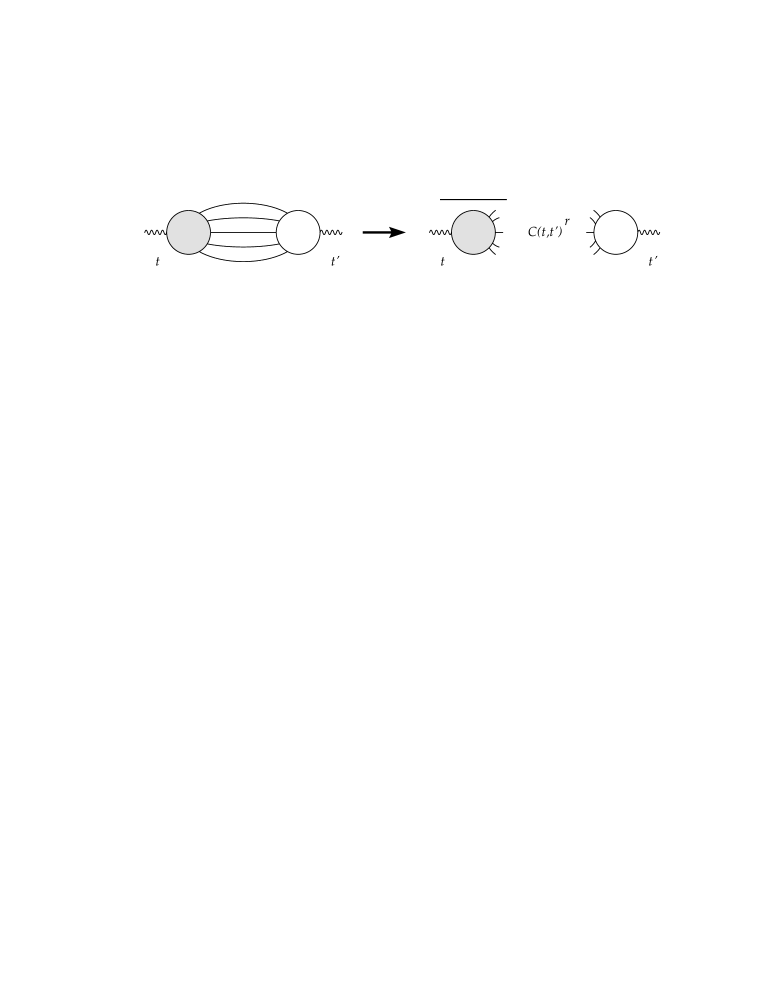
Figure 5: Factorization of generic dynamic self-energy diagram for $t-t^{\prime}\to\infty$.

The overbar on the $1+r$ full vertex means that all external time variables $s_{1},\ldots,s_{r}$ are integrated from $t^{\prime}$ to $t$.

The integration in the $1+r$ full vertex can be done considering first the contribution of all dynamic diagrams that can be generated from a $1+r$ full vertex base diagram $B$ and then summing up the contributions from all possible base diagrams. Neglecting the full-empty vertex connection symmetry factor, the contribution of all dynamic diagram generated by the $1+r$ full vertex base diagram $B$ with $1+E$ external and $I$ internal vertices, can be written as:

$$\int_{t^{\prime}}^{t}\prod_{i=1}^{E}ds_{i}\,\Lambda_{B}(t,s_{1},\ldots,s_{E})\,\prod_{i=1}^{E}\,C(s_{i},t^{\prime})^{n_{i}}\,C(t,t^{\prime})^{n_{0}-1}\,\Lambda^{(0)}(t^{\prime})$$ (31)

where $n_{i}$ is the number of external legs of the $i$-th external bare vertex of $B$, and $\Lambda^{(0)}(t^{\prime})\equiv\Lambda^{(0)}(C(0))$ is the contribution of the $1+r$ empty vertex.

In the limit $t-t^{\prime}\to\infty$ the first term of eq. (31) is not zero only if all $s_{i}\sim t\gg t^{\prime}$ and we can replace all $C(s_{i},t^{\prime})$ in the second term with $C(t,t^{\prime})=C(\infty)$. Equation (31) then factorizes, cfr. Fig. 5, as

$$\Lambda_{B}(t)\,C(t,t^{\prime})^{r}\,\Lambda^{(0)}(t^{\prime})$$ (32)

where

$$\Lambda_{B}(t)=\int_{t^{\prime}}^{t}\prod_{i=1}^{E}ds_{i}\,\left.\Lambda_{B}(s_{0},s_{1},\ldots,s_{E})\right|_{s_{0}=t}.$$ (33)

Finally by adding the appropriate full-empty vertex connection symmetry factor and summing eq. (32) over all possible $1+r$ base diagrams $B$ one recovers the complete dynamic diagram contribution in the limit $t-t^{\prime}\to\infty$ from the $1+r$ vertex to $\Sigma_{\hat{\varphi}\hat{\varphi}}(t,t^{\prime})$.

III.1 $1+r$ full vertex base diagram

From the definition of $\Lambda_{B}(s_{0})$ (33) and the expression (29) it follows that

$$\Lambda_{B}(s_{0})=M(B)\int_{t^{\prime}}^{s_{0}}\prod_{i=1}^{N}\,ds_{i}\,\int\prod_{i=1}^{N}\,d\alpha_{s_{i}}d\overline{\alpha}_{s_{i}}\,\prod_{j=0}^{N}\prod_{i=1}^{N}\,K_{ji}\,C[s_{i}-s_{j}+\overline{\alpha}_{s_{i}}\alpha_{s_{i}}\theta(s_{j}-s_{i})-\overline{\alpha}_{s_{j}}\alpha_{s_{j}}\theta(s_{i}-s_{j})]^{n_{ji}}$$ (34)

where $N=I+E$ is the total number of bare vertices making up $B$, excluding the final one connected to the external $\hat{\varphi}$-leg at time $s_{0}=t$. This expression can be simplified by integrating over $s_{1},\ldots,s_{N}$ in a fixed order because from FDT it follows that:

$$C[x-y+\overline{\alpha}_{x}\alpha_{x}\theta(y-x)-\overline{\alpha}_{y}\alpha_{y}\theta(x-y)]=\left\{\begin{array}[]{ll}C[x-y+\overline{\alpha}_{x}\alpha_{x}\theta(y-x)]&\mbox{if $x<y$}\\ &\\ C[y-x+\overline{\alpha}_{y}\alpha_{y}\theta(x-y)]&\mbox{if $x>y$}\\ \end{array}\right.$$ (35)

Thus ordering $s_{1},\ldots,s_{N}$ so that:

$$(s_{1},\ldots,s_{N})\to(s_{i_{1}},\ldots,s_{i_{N}})\quad:\quad s_{i_{p}}>s_{i_{q}}\quad\mbox{if}\ q>p$$ (36)

the integrand of eq. (34) can be rewritten as

$$\prod_{j=0}^{N}\prod_{i=1}^{N}\,K_{ji}\, \hskip-14.22636ptC[s_{i}-s_{j}+\overline{\alpha}_{s_{i}}\alpha_{s_{i}}\theta(s_{j}-s_{i})-\overline{\alpha}_{s_{j}}\alpha_{s_{j}}\theta(s_{i}-s_{j})]^{n_{ji}}$$ (37)

$$\Rightarrow\prod_{p=1}^{N}\prod_{q<p}^{0,N}\,K_{i_{q}i_{p}}\,C[s_{i_{p}}-s_{i_{q}}+\overline{\alpha}_{s_{i_{p}}}\alpha_{s_{i_{p}}}\theta(s_{i_{q}}-s_{i_{p}})]^{n_{i_{q}i_{p}}}$$

Inserting this expression into (34) and using the identity:

$$\int_{t^{\prime}}^{s_{0}}\,\prod_{i=1}^{N}ds_{i}\equiv\sum_{(i_{1},\ldots,i_{N})\in\mbox{P}(1,\ldots,N)}\int_{t^{\prime}}^{s_{0}}ds_{i_{1}}\int_{t^{\prime}}^{s_{i_{1}}}ds_{i_{2}}\cdots\int_{t^{\prime}}^{s_{i_{N-1}}}ds_{i_{N}}$$ (38)

where $\mbox{P}(1,\ldots,N)$ are the $N!$ permutations of $(1,\ldots,N)$, we end up with

$$\Lambda_{B}(s_{0}) = M(B)\sum_{(i_{1},\ldots,i_{N})\in\mbox{P}(1\ldots,N)}\int_{t^{\prime}}^{s_{0}}ds_{i_{1}}\int_{t^{\prime}}^{s_{i_{1}}}ds_{i_{2}}\cdots\int_{t^{\prime}}^{s_{i_{N-1}}}ds_{i_{N}}$$ (39)

$$\hskip 42.67912pt\times\prod_{p=1}^{N}\left[\int\,d\alpha_{s_{i_{p}}}d\overline{\alpha}_{s_{i_{p}}}\,\prod_{q<p}^{0,N}\,K_{i_{q}i_{p}}\,C[s_{i_{p}}-s_{i_{q}}+\overline{\alpha}_{s_{i_{p}}}\alpha_{s_{i_{p}}}\theta(s_{i_{p}}-s_{i_{q}})]^{n_{i_{q}i_{p}}}\right]$$

The integration over Grassman variables is now diagonal and can be performed. A straightforward algebra leads to

$$\Lambda_{B}(s_{0}) = M(B)\sum_{(i_{1},\ldots,i_{N})\in\mbox{P}(1\ldots,N)}\int_{t^{\prime}}^{s_{0}}ds_{i_{1}}\int_{t^{\prime}}^{s_{i_{1}}}ds_{i_{2}}\cdots\int_{t^{\prime}}^{s_{i_{N-1}}}ds_{i_{N}}\prod_{p=1}^{N}\,\frac{\partial}{\partial s_{i_{p}}}\left[\prod_{q<p}^{0,N}K_{i_{q}i_{p}}\,C(s_{i_{q}},s_{i_{p}})^{n_{i_{q}i_{p}}}\right]$$ (40)

$$= M(B)\sum_{(i_{1},\ldots,i_{N})\in\mbox{P}(1\ldots,N)}\prod_{p=1}^{N}\,\int_{t^{\prime}}^{s_{i_{p}-1}}ds_{i_{p}}\,\frac{\partial}{\partial s_{i_{p}}}\left[\prod_{q=0}^{p-1}K_{i_{q}i_{p}}\,C(s_{i_{q}},s_{i_{p}})^{n_{i_{q}i_{p}}}\right].$$

As simple example of eq. (40) consider the base diagram $B$ shown in Fig. 4. The bare vertices of $B$ are numbered as shown in Fig. 6.

Figure 6: Base diagram vertex numbering.

There are two possible orderings, namely: $\{012\}$ and $\{021\}$. We use the short-hand notation $0$ for $s_{0}$, $1$ for $s_{1}$ and so on. Then from eq. (40) the contribution of this base diagram is

$$\Lambda_{B}(s_{0})=\frac{1}{2}\int_{t^{\prime}}^{0}d1\int_{t^{\prime}}^{1}d2\,\partial_{1}C(0,1)\,\partial_{2}\left[C(0,2)C(1,2)^{2}\right]+\frac{1}{2}\int_{t^{\prime}}^{0}d2\int_{t^{\prime}}^{2}d1\,\partial_{2}C(0,2)\,\partial_{1}\left[C(0,1)C(2,1)^{2}\right]$$ (41)

The factor $1/2$ is the symmetry factor of the base diagram $B$.

In the direct calculation we have to evaluate the three dynamic diagram generated by $B$ shown in Fig. 4 using the dynamic rules and FDT, and then add the results. The first diagram from left, with the vertex numbered as in Fig. 6, leads to:

$$\int_{t^{\prime}}^{0}d1\int_{t^{\prime}}^{1}d2\,G(0,1)G(1,2)C(1,2)C(0,2)=\frac{1}{2}\int_{t^{\prime}}^{0}d1\int_{t^{\prime}}^{1}d2\,\partial_{1}C(0,1)\partial_{2}C(1,2)^{2}C(0,2)$$ (42)

while the second to:

$$\int_{t^{\prime}}^{0}d2\int_{t^{\prime}}^{2}d1\,G(0,2)G(2,1)C(2,1)C(0,1)=\frac{1}{2}\int_{t^{\prime}}^{0}d2\int_{t^{\prime}}^{2}d1\,\partial_{2}C(0,2)\partial_{1}C(2,1)^{2}C(0,1)$$ (43)

and finally the third to:

$$\frac{1}{2}\int_{t^{\prime}}^{0}d1\int_{t^{\prime}}^{0}d2\,G(0,1)G(0,2)C(2,1)^{2}=\frac{1}{2}\int_{t^{\prime}}^{0}d1\int_{t^{\prime}}^{0}d2\,\partial_{1}C(0,1)\partial_{2}C(0,2)C(2,1)^{2}$$ (44)

The factor $1/2$ in the third diagram follows from the symmetry of the diagram. By adding the three contributions, and using the identity

$$\int_{t^{\prime}}^{0}d1\int_{t^{\prime}}^{0}d2=\int_{t^{\prime}}^{0}d1\int_{t^{\prime}}^{1}d2+\int_{t^{\prime}}^{0}d2\int_{t^{\prime}}^{2}d1$$ (45)

one easily recovers the result (41).

We note that all integrations in eq. (41) can be done. Indeed the two integrals in eq. (41) can be combined together to give

$$\Lambda_{B}(s_{0})=\int_{t^{\prime}}^{0}d1\int_{t^{\prime}}^{1}d2\,\partial_{1}C(0,1)\,\partial_{2}\left[C(0,2)C(1,2)^{2}\right]$$ (46)

and performing the integral over $2$ and then over $1$ one ends up with

$$\Lambda_{B}(s_{0})=\frac{1}{2}\Bigl{[}C(0)^{4}-C(0)^{2}\,C(\infty)^{2}-2\,C(0)\,C(\infty)^{3}+2\,C(\infty)^{4}\Bigr{]}$$ (47)

where $C(0)=C(t,t)$ and $C(\infty)=C(t,t^{\prime})$.

The possibility of carrying out all integrals over $s_{i}$ is not a properties of this special example, but it is a general result valid for any base diagram $B$, as shown in the next subsections.

III.2 Recursive integration: sum rules approach

Equation (40) can be written as

$$\Lambda_{B}(s_{0})=\sum_{(i_{1},\ldots,i_{N})\in\mbox{P}(1,\ldots,N)}F_{B}\{s_{0};s_{i_{1}},\ldots,s_{i_{N}}\}$$ (48)

where

$$F_{B}\{s_{0};s_{i_{1}},\ldots,s_{i_{N}}\}=M(B)\prod_{p=1}^{N}\,\int_{t^{\prime}}^{s_{i_{p}-1}}ds_{i_{p}}\,\frac{\partial}{\partial s_{i_{p}}}\left[\prod_{q=0}^{p-1}K_{i_{q}i_{p}}\,C(s_{i_{q}},s_{i_{p}})^{n_{i_{q}i_{p}}}\right]$$ (49)

is contribution of the base diagram $B$ when the time variables $s_{1},\ldots,s_{N}$ are ordered as $(s_{i_{1}},\ldots,s_{i_{N}})$, see eq. (36). We shall denote this ordered base diagram by $B\{s_{0},s_{i_{1}},\ldots,s_{i_{N}}\}$

The sum (48) can be performed by first selecting all terms where the pair $(i_{N-1},i_{N})$ is equal to $(h,k)$ or $(k,h)$, and then summing over all possible distinct index pairs $h,k$. If we do this we end up with

$$\Lambda_{B}(s_{0})=\sum_{(h,k)}\sum_{(i_{1},\ldots,i_{N-2})\in\mbox{P}[(1\ldots,N)-(h,k)]}\Bigl{[}F_{B}\{s_{0};s_{i_{1}},\ldots,s_{i_{N-2}},s_{h},s_{k}\}+F_{B}\{s_{0};s_{i_{1}},\ldots,s_{i_{N-2}},s_{k},s_{h}\}\Bigr{]}$$ (50)

where the first sum is over all distinct pairs $(h,k)$ with $h,k=1,\ldots,N$, while the second sun over is all permutations of $(1,\ldots,N)$ once $h$ and $k$ are taken out.

From eq. (49) it is easy to realize that the two terms in square brackets differ only for the last two integrals over $s_{h}$ and $s_{k}$, so that we have to evaluate the sum:

$$\int_{t^{\prime}}^{s_{i_{N-2}}}ds_{h}\,\partial_{s_{h}}\left[\prod_{q=0}^{N-2}K_{i_{q}h}\,C(s_{i_{q}},s_{h})^{n_{i_{q}h}}\right]\int_{t^{\prime}}^{s_{h}}ds_{k}\,\partial_{s_{k}}\left[\prod_{q=0}^{N-2}K_{i_{q}k}\,C(s_{i_{q}},s_{k})^{n_{i_{q}k}}\,K_{hk}\,C(s_{h},s_{k})^{n_{hk}}\right]+(h\leftrightarrow k)$$ (51)

where the second term is obtained from the first by exchanging $s_{h}$ and $s_{k}$.

By performing the $s_{k}$ integral in the first term and the $s_{h}$ integral in the second term and rearranging the terms we obtain the sum rule

$$F_{B}\{\ldots,s_{h},s_{k}\}+F_{B}\{\ldots,s_{k},s_{h}\}=F_{B}\{\ldots,s_{h}|s_{k}=s_{h}\}-F_{B}\{\ldots,s_{h}|s_{k}=t^{\prime}\}-F_{B}\{\ldots,s_{k}|s_{h}=t^{\prime}\}$$ (52)

where the dots “$...$” is the short hand notation for “$s_{0};s_{i_{1}},\ldots,s_{i_{N-2}}$”. The term $F_{B}\{...,s_{h}|s_{k}=s_{h}\}$ is the contribution of the ordered base diagram $B\{s_{0},s_{i_{1}},\ldots,s_{i_{N-2}},s_{h}|s_{k}=s_{h}\}$ obtained from $B\{s_{0},s_{i_{1}},\ldots,s_{i_{N-2}},s_{h},s_{k}\}$ by setting $s_{k}=s_{h}$, i.e., by replacing all lines connecting vertices $h$ and $k$ by $C(s_{h},s_{h})=C(0)$. This reduces the number of integrations by one since the vertices $h$ and $k$ “collapse” into a single composite or effective vertex. Similarly $F_{B}\{...,s_{h}|s_{k}=t^{\prime}\}$ is the contribution of the ordered base diagram $B\{s_{0},s_{i_{1}},\ldots,s_{i_{N-2}},s_{h}|s_{k}=t^{\prime}\}$ obtained from $B\{s_{0},s_{i_{1}},\ldots,s_{i_{N-2}},s_{h},s_{k}\}$ by setting $s_{k}=t^{\prime}$, i.e., by replacing all lines connecting the vertex $k$ to any other vertex $i\not=k$ of $B$ by $C(s_{i},t^{\prime})=C(\infty)$. Also in this case the number of integrations is reduced by one since the vertex $k$ is “removed” from the diagram. $F_{B}\{...,s_{k}|s_{h}=t^{\prime}\}$ is defined in a similar way.

This procedure can be repeated by considering triples $(l,h,k)$ of vertices and writing

$$\Lambda_{B}(s_{0})=\sum_{(l,h,k)}\sum_{(i_{1},\ldots,i_{N-3})\in\mbox{P}[(1\ldots,N)-(l,h,k)]}\sum_{\mbox{P}(l,h,k)}\,F_{B}\{s_{0};s_{i_{1}},\ldots,s_{i_{N-3}},s_{l},s_{h},s_{k}\}$$ (53)

where now the first sum runs over all distinct triplets $(l,h,k)$, the second over all possible permutations of $(1,\ldots,N)$ once the triplet $(l,h,k)$ has been removed and the last over the six permutations of the triplet $(l,h,k)$.

By using the sum rule (52) the last sum can be written as

$$\sum_{\mbox{P}(l,h,k)}\,F_{B}\{\ldots,s_{l},s_{h},s_{k}\} =$$ (54)

$$\phantom{+}\hskip-85.35826ptF_{B}\{\ldots,s_{l},s_{h}|s_{k}=s_{h}\}-F_{B}\{\ldots,s_{l},s_{h}|s_{k}=t^{\prime}\}-F_{B}\{\ldots,s_{l},s_{k}|s_{h}=t^{\prime}\}$$

$$\hskip-85.35826pt+F_{B}\{\ldots,s_{h},s_{k}|s_{l}=s_{k}\}-F_{B}\{\ldots,s_{h},s_{k}|s_{l}=t^{\prime}\}-F_{B}\{\ldots,s_{h},s_{l}|s_{k}=t^{\prime}\}$$

$$\hskip-85.35826pt+F_{B}\{\ldots,s_{k},s_{l}|s_{h}=s_{l}\}-F_{B}\{\ldots,s_{k},s_{l}|s_{h}=t^{\prime}\}-F_{B}\{\ldots,s_{k},s_{h}|s_{l}=t^{\prime}\}$$

The three term with positive sign can be combined together and give

$$F_{B}\{\ldots,s_{l},s_{h}|s_{k}=s_{h}\}+F_{B}\{\ldots,s_{h},s_{k}|s_{l}=s_{k}\}+F_{B}\{\ldots,s_{k},s_{l}|s_{h}=s_{l}\} =$$ (55)

$$\hskip-256.0748pt\phantom{-}F_{B}\{\ldots,s_{l}|s_{h}=s_{l},s_{k}=s_{h}\}$$

$$\hskip-256.0748pt-F_{B}\{\ldots,s_{l}|s_{h}=t^{\prime},s_{k}=s_{h}\}-F_{B}\{\ldots,s_{h}|s_{k}=t^{\prime},s_{l}=s_{k}\}-F_{B}\{\ldots,s_{k}|s_{l}=t^{\prime},s_{h}=s_{l}\}$$

The term $F_{B}\{\ldots,s_{l}|s_{h}=s_{l},s_{k}=s_{h}\}$ is the contribution of the ordered diagram $B\{\ldots,s_{l}|s_{h}=s_{l},s_{k}=s_{h}\}$ obtained from $B\{\ldots,s_{l},s_{h}|s_{k}=s_{h}\}$ by setting $s_{h}=s_{l}$, or equivalently from $B\{\ldots,s_{l},s_{h},s_{k}\}$ by setting $s_{k}=s_{h}$ and $s_{h}=s_{l}$. In both cases the number of integrations is reduced by two and all lines connecting the three vertices are replaced by $C(0)$.

The term $F_{B}\{\ldots,s_{l}|s_{h}=t^{\prime},s_{k}=s_{h}\}$ is the contribution of the ordered diagram $B\{\ldots,s_{l}|s_{h}=t^{\prime},s_{k}=s_{h}\}$ obtained from $B\{\ldots,s_{l},s_{h}|s_{k}=s_{h}\}$ by setting $s_{h}=t^{\prime}$, or equivalently from $B\{\ldots,s_{l},s_{h},s_{k}\}$ by setting $s_{k}=s_{h}$ first and then $s_{h}=t^{\prime}$. This means that all lines connecting the vertices $h$ and $k$ are replaced by $C(0)$ while all lines connecting either vertex $h$ or $k$ with any other vertex $i\not=h,k$ by $C(\infty)$, reducing at the same time the number of integrations by two. The other two terms are obtained in a similar way.

Finally the six terms in (54) with negative sign can be evaluated in pairs using the sum rule (52). One then gets, for example,

$$F_{B}\{\ldots,s_{l},s_{h}|s_{k}=t^{\prime}\}+F_{B}\{\ldots,s_{h},s_{l}|s_{k}=t^{\prime}\} =$$ (56)

$$\hskip-156.49014pt\phantom{-}F_{B}\{\ldots,s_{l}|s_{h}=s_{l},s_{k}=t^{\prime}\}-F_{B}\{\ldots,s_{l}|s_{h}=t^{\prime},s_{k}=t^{\prime}\}-F_{B}\{\ldots,s_{h}|s_{l}=t^{\prime},s_{k}=t^{\prime}\}$$

Even if the notation should be now clear it is useful to stress that $F_{B}\{\ldots,s_{l}|s_{h}=s_{l},s_{k}=t^{\prime}\}$ is the contribution from the ordered diagram $B\{\ldots,s_{l}|s_{h}=s_{l},s_{k}=t^{\prime}\}$ obtained from $B\{\ldots,s_{l},s_{h}|s_{k}=t^{\prime}\}$ by setting $s_{h}=s_{l}$, or equivalently from $B\{\ldots,s_{l},s_{h},s_{k}\}$ by setting $s_{k}=t^{\prime}$ first and only then $s_{h}=s_{l}$. Similarly $F_{B}\{\ldots,s_{l}|s_{h}=t^{\prime},s_{k}=t^{\prime}\}$ is the contribution from the ordered diagram $B\{\ldots,s_{l}|s_{h}=t^{\prime},s_{k}=t^{\prime}\}$ obtained from $B\{\ldots,s_{l},s_{h}|s_{k}=t^{\prime}\}$ by setting $s_{h}=t^{\prime}$, or equivalently from $B\{\ldots,s_{l},s_{h},s_{k}\}$ by setting $s_{k}=t^{\prime}$ and only then $s_{h}=t^{\prime}$. The order in the construction is relevant since, for example, $F_{B}\{\ldots,s_{l}|s_{h}=t^{\prime},s_{k}=t^{\prime}\}$ is in general different from $F_{B}\{\ldots,s_{l}|s_{h}=t^{\prime},s_{k}=s_{h}\}$.

Collecting all terms we end up with the sum rule:

$$\sum_{\mbox{P}(l,h,k)}\,F_{B}\{\ldots,s_{l},s_{h},s_{k}\} =$$ (57)

$$\hskip-56.9055pt\phantom{-}F_{B}\{\ldots,s_{l}|s_{h}=s_{l},s_{k}=s_{h}\}$$

$$\hskip-56.9055pt-F_{B}\{\ldots,s_{l}|s_{h}=t^{\prime},s_{k}=s_{h}\}-F_{B}\{\ldots,s_{h}|s_{k}=t^{\prime},s_{l}=s_{k}\}-F_{B}\{\ldots,s_{k}|s_{l}=t^{\prime},s_{h}=s_{l}\}$$

$$\hskip-56.9055pt-F_{B}\{\ldots,s_{l}|s_{h}=s_{l},s_{k}=t^{\prime}\}+F_{B}\{\ldots,s_{l}|s_{h}=t^{\prime},s_{k}=t^{\prime}\}+F_{B}\{\ldots,s_{h}|s_{l}=t^{\prime},s_{k}=t^{\prime}\}$$

$$\hskip-56.9055pt-F_{B}\{\ldots,s_{h}|s_{k}=s_{h},s_{l}=t^{\prime}\}+F_{B}\{\ldots,s_{h}|s_{k}=t^{\prime},s_{l}=t^{\prime}\}+F_{B}\{\ldots,s_{k}|s_{h}=t^{\prime},s_{l}=t^{\prime}\}$$

$$\hskip-56.9055pt-F_{B}\{\ldots,s_{k}|s_{l}=s_{k},s_{h}=t^{\prime}\}+F_{B}\{\ldots,s_{k}|s_{l}=t^{\prime},s_{h}=t^{\prime}\}+F_{B}\{\ldots,s_{l}|s_{k}=t^{\prime},s_{h}=t^{\prime}\}$$

that, when inserted into eq. (53), eliminates two time integrations and replaces the lines connected with the vertex integrated out by either $C(0)$ or $C(\infty)$.

The procedure can be iterated to build sum rules for four vertices, five vertices and so. Despite the fact that the derivation of the sum rules for any number of vertices is straightforward we shall not push it here because these can be more easily obtained using the diagrammatic rules of next subsection.

By using iteratively the sum rules and

$$F_{B}\{s_{0};s|\ldots\}=F_{B}\{s_{0}|s=t,\ldots\}-F_{B}\{s_{0}|s=t^{\prime},\ldots\}$$ (58)

all $N$ time integrals in $\Lambda_{B}(s_{0})$ can be eliminated in turn in favor of $C(0)$ and $C(\infty)$. This concludes the proof that for any base diagram $B$ all time integrals can be performed and moreover

$$\Lambda_{B}(s_{0})\equiv\Lambda_{B}(C(0),C(\infty))$$ (59)

where $\Lambda_{B}(x,y)$ is a function that depends only on the topology of $B$.

To illustrate the sum rule approach we conclude this subsection by reconsidering the simple example of Fig. 6. For this diagram $N=2$, therefore from eq. (50) and the sum rule (52) it follows

$$\Lambda_{B}(s_{0}) = F_{B}\{0;1,2\}+F_{B}\{0;2,1\}$$ (60)

$$= F_{B}\{0;1|2=1\}-F_{B}\{0;1|2=t^{\prime}\}-F_{B}\{0;2|1=t^{\prime}\}.$$

By using now the sum rule (58) we end up with

$$\Lambda_{B}(s_{0}) = \phantom{-}F_{B}\{0|1=0,2=1\}-F_{B}\{0|1=t^{\prime},2=1\}$$

$$-F_{B}\{0|1=0,2=t^{\prime}\}+F_{B}\{0|1=t^{\prime},2=t^{\prime}\}$$

$$-F_{B}\{0|2=0,1=t^{\prime}\}+F_{B}\{0|2=t^{\prime},1=t^{\prime}\}.$$

which for the diagram of Fig. 6 leads to

$$\Lambda_{B}(s_{0}) = \frac{1}{2}\Bigl{[}C(0)^{4}-C(0)^{2}C(\infty)^{2}-C(\infty)^{3}C(0)+C(\infty)^{4}-C(\infty)^{3}C(0)+C(\infty)^{4}\Bigr{]}$$ (62)

$$= \frac{1}{2}\Bigl{[}C(0)^{4}-C(0)^{2}\,C(\infty)^{2}-2\,C(0)\,C(\infty)^{3}+2\,C(\infty)^{4}\Bigr{]}$$

One easily recognizes the result (47) from the direct calculation.

III.3 Recursive integration: diagrammatic approach

While the integration based on sum rules described in the previous subsection can be carried on for any base diagram $B$, in practical calculations it can become quite cumbersome. Thus it would be desirable to have a simpler way of proceeding. In general diagrammatic methods are simpler and more transparent, for this reason in this subsection we present the diagrammatic approach that allow for a graphical integration directly on the base diagram $B$.

The diagrammatic integration goes through the following steps:

$\bullet$ Time Ordering
The first step is to generate all possible ordered base diagrams $B\{s_{0},s_{i_{1}},\ldots,s_{i_{N}}\}$ by considering all possible permutations $(i_{1},\ldots,i_{N})\in\mbox{P}(1,\ldots,N)$. Once the time order of $B$ has been fixed, each ordered diagram $B\{s_{0},s_{i_{1}},\ldots,s_{i_{N}}\}$ is decorated by orienting each line connecting two vertices by drawing an arrow in the direction of the time flow, i.e., pointing from the shortest to the largest time.

The expression of $F_{B}\{s_{0};s_{i_{1}},\ldots,s_{i_{N}}\}$ is recovered by first assigning to each line of the oriented diagram $B\{s_{0},s_{i_{1}},\ldots,s_{i_{N}}\}$ the correlation function $C(s_{i_{p}},s_{i_{q}})$, where $i_{p}$ and $i_{q}$ are the labels of the two vertices connected by the line, and then taking the product for $p=1,\ldots,N$ of the derivative with respect to $s_{i_{p}}$ of the product of the correlation functions $C(s_{i_{q}},s_{i_{p}})$ associated with all outgoing oriented lines originating from vertex $i_{p}$. Finally $F_{B}\{s_{0};s_{i_{1}},\ldots,s_{i_{N}}\}$ follows by integrating the result over all $s_{i_{p}}$ starting from $s_{i_{N}}$ and proceeding towards $s_{i_{1}}$ in order [cfr. eq. (49)]. In each diagram the integration starts from the vertex with the shortest time. By construction this vertex has only outgoing oriented lines, and there is only one of such vertex in each diagram. The integration cancels the arrows from all oriented lines originating from the vertex we are integrating on, and replace the original diagram by two new diagrams. Thus we have the following graphical integration rule.

$\bullet$ Time Integration

1. In each diagram peak up the vertex with only outgoing oriented lines and replace the original diagram by the two diagrams obtained as follows:

   Diagram $1$: Assign to the vertex with only outgoing oriented lines the next shortest time, i.e., $s_{i_{p}}\to s_{i_{p-1}}$. If the vertex $i_{p-1}$ is not directly connected to $i_{p}$ draw a dotted line between the two vertices to remember they have the same time. Next replace all outgoing oriented lines with simple not-oriented lines drawing them as: full line if the line connects two vertices at different time; dashed line if the line connects two vertices at the same time. As before, we shall call effective vertex the group of bare vertices with equal time, i.e., the group of vertices connected by dashed or dotted lines.

   Diagram $2$: Set the time of the vertex with only outgoing oriented lines to $t^{\prime}$ and replace all outgoing oriented lines of the vertex by cutted lines, i.e., replace the arrow by the “cut” sign “$/$”. Finally multiply the diagram by $-1$ so that two new diagrams contribute with opposite signs.

2. Merge all diagrams that differ only for the oriented outgoing lines originating from the same effective vertex into the single diagram obtained from any one of them by orienting all not-oriented full lines originating from the effective vertex according to the orientation of all diagrams we are merging to. This leaves us with diagrams made of only oriented lines (arrows), dashed or dotted lines and cutted lines.

It is not difficult to realize that this rule produces diagrams where the vertex, or effective vertex, with the shortest time has only outgoing oriented lines. Moreover the vertices connected via cutted lines do not contribute anymore to the integration process. The procedure can then be iterated untill one is left with diagrams made of only dashed or cutted lines. The dotted lines are used for time bookkeeping and can be eliminated if not needed.

$\bullet$ Value of diagrams
The value of $\Lambda_{B}(s_{0})$ is obtained by evaluating each final diagram with dashed lines replaced by the equal time correlation function $C(t,t)=C(0)$ and cutted lines by the infinite time correlation function $C(t,t^{\prime})=C(\infty)$, and summing up all contributions from different diagrams with the appropriate plus or minus sign.

To illustrate the graphical integration rules we consider again the base diagram shown in Fig. 6. The two possible oriented diagrams $B\{012\}$ and $B\{021\}$ are shown in Figs. 7 and 8 together with the result of step $1)$ of the time integration rule.

Figure 7: Oriented base diagram $B\{012\}$ and result of first diagrammatic integration.

Figure 8: Oriented base diagram $B\{021\}$ and result of first diagrammatic integration.

The diagrams $(a)$ in Fig. 7 and $(c)$ in Fig. 8 differs only for the orientation of the outgoing lines originating from the effective vertex made by the bare vertices $1$ and $2$. The two diagrams are then merged together into the diagram shown in Fig. 9, step $2)$ of the time integration rule.

Figure 9: Merging of diagram $(a)$ of Fig. 7 and diagram $(c)$ of Fig. 8.

Diagrams $(b)$ of Fig. 7, $(d)$ of Fig. 8 and $(e)$ of Fig. 9 contain only (effective) vertices with all outgoing lines or connected by cutted lines, thus the time integration steps $1)$ and $2)$ can be repeated for each one of these diagrams. This second round eliminates all oriented lines and, taking into account the $-1$ signs, $\Lambda_{B}(s_{0})$ is given by the sum of the six diagrams shown in Fig. 10.

Figure 10: Final diagrams.

Evaluating these diagrams and multiplying the result by the symmetry factor $M(B)=1/2$ of the base diagram, we and up with

$$\Lambda_{B}(s_{0}) = \frac{1}{2}\Bigl{[}C(0)^{4}-C(0)^{2}\,C(\infty)^{2}-C(0)\,C(\infty)^{3}+C(\infty)^{4}-C(0)\,C(\infty)^{3}+C(\infty)^{4}\Bigl{]}$$ (63)

$$= \frac{1}{2}\Bigl{[}C(0)^{4}-C(0)^{2}\,C(\infty)-2\,C(0)\,C(\infty)^{3}+2\,C(\infty)^{4}\Bigr{]},$$

i.e., again the result (47) obtained previously by direct integration.

IV The replica calculation

IV.1 The $1+r$ full vertex base diagram

In the previous Section we have shown that in the limit $t-t^{\prime}\to\infty$ the contribution $\Lambda_{B}(t)$ of the $1+r$ base vertex $B$ to the $1+r$ full vertex can be obtained by considering all possible diagrams that can be constructed from $B$ by replacing the lines connecting the bare vertices by either dashed or cutted lines in all possible ways. Clearly there are some constraints to be considered, for example all lines connecting the same pair of vertices must be replaced simultaneously. In other words it not possible to have dashed and cutted line connecting the same pair of vertices, see e.g. Fig. 10.

Given any base diagram $B$ a simple way of generating all allowed diagrams is that of attaching to each bare vertex $i=0,1,\ldots,N$ of $B$ a label $a_{i}$. Each label can take the values $1,\ldots,n$, where $n$ is an arbitrary integer. The next step is that of introducing the “projector” operators $\delta_{a_{i}a_{j}}$ and $(1-\delta_{a_{i}a_{j}})$ and associate to each line of $B$ connecting the vertex $i$ and vertex $j$ the “correlation” function

$$C_{a_{i}a_{j}}=C(0)\,\delta_{a_{i}a_{j}}+C(\infty)\,(1-\delta_{a_{i}a_{j}})$$ (64)

By representing the projector $\delta_{a_{i}a_{j}}$ with a dashed line and the projector $(1-\delta_{a_{i}a_{j}})$ with a cutted line it is easy to convince oneself that the sum over all $a_{i}$ ($i=1,\ldots,N$) from $1$ to $n$ generates all possible diagrams that can be constructed from $B$.

The interesting point of this method is that it does not only generates all possible diagrams but, as a “bonus”, it also gives the correct weight and sign for each one of them. For a single line this is rather trivial since for $n\to 0$ one has the formal identity:

$$\int_{t^{\prime}}^{t}ds\,\frac{\partial}{\partial s}\,C(t,s)=C(0)-C(\infty)\equiv\lim_{n\to 0}\sum_{b=1}^{n}C_{ab}$$ (65)

that ensures that for $n\to 0$ an oriented line is not only replaced by a dashed line and a cutted line, but also that the second one comes with a negative relative sign. By using the properties of the projection operators this identity can be extended to a bunch of oriented lines connecting two vertices.

In the Appendix A we show that the sum over labels $a_{i}$ with $i=1,\ldots,N$ for any base diagram $B$ reproduces in $n\to 0$ limit the sum rules discussed in Sec. III.2. This implies that $\Lambda_{B}(s_{0})$ can be expressed in the “replica” form

$$\Lambda_{B}(t)=M(B)\,\lim_{n\to 0}\sum_{a_{1},\ldots,a_{N}}^{1,n}\prod_{i=1}^{N}\prod_{j=0}^{i-1}K_{ij}\,C_{a_{i}a_{j}}^{n_{ij}}$$ (66)

We then have the following simple rule to evaluate $\Lambda_{B}(s_{0})$:

1. Given a base diagram $B$ assign to each bare vertex $i=0,\ldots,N$ of $B$ a “replica” index $a_{i}$.

2. Assign to each line connecting the vertices $i$ and $j$ the correlation function $C_{a_{i}a_{j}}$ given in eq. (64).

3. Sum over all replica indexes $a_{i}$ with $i=1,\ldots,N$ from $1$ to $n$ and multiply the result by the diagram symmetry factor $M(B)$.

4. Take the limit $n\to 0$ of the result.

To illustrate the procedure, i.e., formula (66), we consider again the base diagram shown in Fig. 6. For this diagram eq. (66) reads:

$$\Lambda_{B}(t) = \frac{1}{2}\lim_{n\to 0}\sum_{a_{1}=1}^{n}\sum_{a_{2}=1}^{n}C_{a_{0}a_{1}}\,C_{a_{0}a_{2}}\,C_{a_{1}a_{2}}^{2}$$ (67)

$$= \frac{1}{2}\lim_{n\to 0}\left[C(0)^{4}+(n-1)C(0)^{2}C(\infty)^{2}+2(n-1)C(0)\,C(\infty)^{3}+(n-1)(n-2)C(\infty)^{4}\right]$$

$$= \frac{1}{2}\left[C(0)^{4}-C(0)^{2}C(\infty)^{2}-2C(0)\,C(\infty)^{3}+2C(\infty)^{4}\right]$$

We note that the sum produces all not-equivalent diagrams shown of Fig. 10. Indeed the first term in the second line that follows from $a_{2}=a_{1}=a_{0}$ corresponds to the first diagram shown in Fig. 10. The weight $1$ reflects the fact that there is only one possible choice $a_{2}=a_{1}=a_{0}$. Similarly the second term obtained for $a_{2}=a_{1}\not=a_{0}$ corresponds to the second diagram in Fig. 10. There are $n-1$ choices that satisfy the constraint $a_{2}=a_{1}\not=a_{0}$. The third term follows from either $a_{1}=a_{0}\not=a_{2}$ or $a_{1}\not=a_{0}=a_{2}$ and indeed corresponds to the third and fifth diagrams of Fig. 10. In both cases there are $n-1$ choices that satisfy the constraint. Finally the last term is obtained by taking all three indexes $a_{0},a_{1}$ and $a_{2}$ different from each others, and hence $(n-1)(n-2)$ possible choices. This term corresponds to the fourth (or the equivalent sixth) diagram of Fig. 10.

IV.2 The self-energy diagrams

To finalize the calculation of the self-energy diagrams (15) in the limit $t-t^{\prime}\to\infty$ we also need the contribution from the empty vertex, the quantity $\Lambda^{(0)}(t^{\prime})$ in eq. (32). The empty vertex is given by the equilibrium diagrams of the associated static theory described by the canonical distribution (4), as a consequence the empty vertex is made by the base diagrams used to construct the full-vertex with all lines equal to the equal-time correlation $C(0)$.

The contribution from any one of such diagram $B$ to the empty vertex can be readily written in the replica formalism:

$$\Lambda_{B}^{(0)}(t^{\prime})=M(B)\prod_{i=1}^{N}\prod_{j=0}^{i-1}K_{ij}\,C_{aa}^{n_{ij}}$$ (68)

where we used the same vertex numbering convention as the full vertex diagrams. The limit $n\to 0$ is not necessary since we are only using the diagonal part of $C_{ab}$.

By using the representations (66) and (68) the contribution $\Lambda_{B_{f}B_{e}}^{(r)}(t,t^{\prime})$ of the self-energy diagram with the $1+r$ full vertex generated by the base diagram $B_{f}$ and the $1+r$ empty vertex generated by the base diagram $B_{e}$ reads in the limit $t-t^{\prime}\to\infty$, see eq. (32),

$$\Lambda_{B_{f}B_{e}}^{(r)}(t,t^{\prime})=M(B_{f})\,M(B_{e})\,M(B_{f},B_{e})\lim_{n\to 0}\sum_{a_{1},\ldots,a_{N}}^{1,n}\prod_{i=1}^{N_{f}}\prod_{j=0}^{i-1}K^{f}_{ij}\,C_{a_{i}a_{j}}^{n^{f}_{ij}}\,C(\infty)^{r}\,\prod_{i=1}^{N_{e}}\prod_{j=0}^{i-1}K^{e}_{ij}\,C_{bb}^{n^{e}_{ij}}$$ (69)

where $M(B_{f},B_{e})$ is the symmetry factor generated by the connections between the two vertices.

The term $C(\infty)^{r}$ follows from the lines connecting the $1+E_{f}$ external vertices of $B_{f}$ to the $1+E_{e}$ external vertices of $B_{e}$. Thus by assuming that the replica indexes $a_{i}$ of $B_{f}$ never take a value equal to that of the replica index $b$ of $B_{e}$ this term can be written as

$$C(\infty)^{r}\Rightarrow\prod_{i=0}^{E_{f}}\prod_{j=0}^{E_{e}}J_{ij}\,C_{a_{i}b}^{m_{ij}}$$ (70)

where the rectangular symmetric matrices $J_{ij}$ and $m_{ij}$ give the topology of the connections between $B_{f}$ and $B_{e}$, i.e., $J_{ij}=1$ if the two external vertices are connected or $0$ otherwise, while $m_{ij}=1,2,\ldots$ ($\sum_{ij}m_{ij}=r$) gives the number of lines between the two vertices.

The values of the replica indexes of the two vertices can be made different either assuming $b=n+1$ or forcing the two sets of replicas to assume different values by adding the projectors $(1-\delta_{a_{i}b})$. This second method is more appealing since it maintains the symmetry of replica index, the little price to pay is that now the replica index of diagram $B_{f}$ can take only $n-1$ values, so the limit must be changed from $n\to 0$ to $n\to 1$.

Collection all terms we end up with

$$\Lambda_{B_{f}B_{e}}^{(r)}(t,t^{\prime}) = M(B_{f})\,M(B_{e})\,M(B_{f},B_{e})\lim_{n\to 1}\sum_{a_{1},\ldots,a_{N}}^{1,n}\left[\prod_{i=1}^{N_{f}}\prod_{j=0}^{i-1}K^{f}_{ij}\,C_{a_{i}a_{j}}^{n^{f}_{ij}}\right]\,\left[\prod_{i=0}^{E_{f}}(1-\delta_{a_{i}b})\prod_{j=0}^{E_{e}}J_{ij}\,C_{a_{i}b}^{m_{ij}}\right]$$ (71)

$$\phantom{=======================}\times\left[\prod_{i=1}^{N_{e}}\prod_{j=0}^{i-1}K^{e}_{ij}\,C_{bb}^{n^{e}_{ij}}\right]$$

In Sect. II.2 we have seen that the equilibrium dynamic diagrams for $\Sigma_{\hat{\varphi}\hat{\varphi}}(t,t^{\prime})$ can be obtained by dividing a suitable base diagram with the same topology of the equilibrium dynamic diagrams into two sub-diagrams, one leading to $B_{f}$ and the other to $B_{e}$. This is precisely the role of the projector $\prod_{i=0}^{E_{f}}(1-\delta_{a_{i}b})$ in eq. (71). The total contribution from the self-energy base diagram $B$ is now obtained by considering all possible divisions of $B$ into $B_{f}$ and $B_{e}$ and summing up the result. It is not difficult to realize that all possible distributions of the bare vertices of $B$ between $B_{f}$ and $B_{e}$ can be generated by considering all possible insertions of the projector $\prod_{i=0}^{E_{f}}(1-\delta_{a_{i}b})$. As a consequence the total contribution $\Sigma_{\hat{\varphi}\hat{\varphi}}^{(B)}(t,t^{\prime})$ to the self-energy from all equilibrium diagrams generated by the base diagram $B$ in the limit $t-t^{\prime}\to\infty$ reads

$$\Sigma_{\hat{\varphi}\hat{\varphi}}^{(B)}(t,t^{\prime})=M(B)\lim_{n\to 1}\sum_{a_{1},\ldots,a_{N}}\prod_{i=1}^{N+1}\prod_{j=0}^{i-1}K_{ij}\,C_{a_{i}a_{j}}^{n_{ij}}\,\left(1-\delta_{a_{0}a_{N+1}}\right)$$ (72)

where we have associated the index $0$ with the external vertex at $t$ and the index $N+1$ to the external vertex at $t^{\prime}$ so that the total number of bare vertices of $B$ is $N+2$.

The formula has a simple meaning: to obtain the contribution from all diagrams generated by the self-energy base diagram $B$ just attach to each vertex of $B$ a replica index $a$ and to each line connecting the vertex $a$ and $b$ the correlation function $C_{ab}$ [eq. (64)]. Then sum over all replica indexes from $1$ to $n$ keeping the replica index of the vertices attached to the $t$ and $t^{\prime}$ external legs fixed and different from each other. At the end take the limit $n\to 1$.

To illustrate the procedure we consider the base diagram $B$ shown in Fig. 3. Equation (72), with the symmetry factor $M(B)=1/4$, gives

$$\Sigma_{\hat{\varphi}\hat{\varphi}}^{(3)}(t,t^{\prime}) = \frac{1}{4}\lim_{n\to 1}\sum_{a_{1}=1}^{n}C_{a_{0}a_{1}}^{2}\,C_{a_{0}a_{2}}\,C_{a_{1}a_{2}}^{2}\,(1-\delta_{a_{0}a_{2}})$$ (73)

$$= \frac{1}{4}\lim_{n\to 1}\left[2\,C(0)^{2}\,C(\infty)^{3}+(n-2)\,C(\infty)^{5}\right]$$

$$= \frac{1}{4}\left[2\,C(0)^{2}\,C(\infty)^{3}-\,C(\infty)^{5}\right].$$

The base diagram of Fig. 3 produces the equilibrium dynamic diagrams shown in Fig. 2 whose value is given by eq. (20). Evaluating the integral for $t-t^{\prime}\to\infty$ we indeed have

$$\Sigma_{\hat{\varphi}\hat{\varphi}}^{(3)}(t,t^{\prime}) = \frac{1}{2}\int_{t^{\prime}}^{t}ds\,\frac{\partial}{\partial s}C(t,s)\ C(t,s)C(\infty)^{3}+\frac{1}{4}C(0)^{2}\,C(\infty)^{3}$$ (74)

$$= \frac{1}{4}\left[C(0)^{2}-C(\infty)^{2}\right]\,C(\infty)^{3}+\frac{1}{4}C(0)^{2}\,C(\infty)^{3}$$

$$= \frac{1}{4}\left[2\,C(0)^{2}\,C(\infty)^{3}-\,C(\infty)^{5}\right].$$

Figure 11: Fourth order crossed self-energy base diagram.

As further example consider the base diagram of Fig. 11. This diagram has a symmetry factor of $1/2$, thus the replica calculation gives

$$\Sigma_{\hat{\varphi}\hat{\varphi}}^{(4c)}(t,t^{\prime}) = \frac{1}{2}\lim_{n\to 1}\sum_{a_{1}=1}^{n}\sum_{a_{2}=1}^{n}C_{a_{0}a_{1}}\,C_{a_{0}a_{2}}\,C_{a_{1}a_{2}}^{2}\,C_{a_{0}a_{3}}\,C_{a_{1}a_{3}}\,C_{a_{2}a_{3}}(1-\delta_{a_{0}a_{3}})$$ (75)

$$= \frac{1}{2}\lim_{n\to 1}\left[2\,C(0)^{4}\,C(\infty)^{3}+n\,C(0)^{2}\,C(\infty)^{5}+4(n-2)\,C(0)\,C(\infty)^{6}+(n-2)(n-3)\,C(\infty)^{7}\right]$$

$$= \frac{1}{2}\left[2\,C(0)^{4}\,C(\infty)^{3}+C(0)^{2}\,C(\infty)^{5}-4\,C(0)\,C(\infty)^{6}+2\,C(\infty)^{7}\right]$$

The direct calculation of the equilibrium dynamic diagrams generated by this base diagram is shown in Appendix B.

IV.3 The replicated system and the bifurcation equation

The self-energy base diagram $B$ are the static self-energy diagrams generated by the Hamiltonian $H$ of the associated equilibrium static theory described by the canonical distribution (4). Thus from the results discussed so far it follows that

$$\lim_{t-t^{\prime}\to\infty}\Sigma_{\hat{\varphi}\hat{\varphi}}(t,t^{\prime})=\lim_{n\to 1}\Sigma_{ab},\qquad a\not=b$$ (76)

where $\Sigma_{ab}$ is the static self-energy of the $n$ times replicated system described by the Hamiltonian ${\cal H}_{n}=\sum_{a=1}^{n}H[\varphi_{a}]$ and the 1RSB correlation function [eq. (64)]

$$C_{ab}=\langle\varphi_{a}\varphi_{b}\rangle_{\rm eq}=C(0)\,\delta_{ab}+C(\infty)\,(1-\delta_{ab})$$ (77)

with $C(0)=C(t,t)$ the equal time value of the equilibrium two time correlation function $C(t,t^{\prime})$ and $C(\infty)$ its $t-t^{\prime}\to\infty$ limit. The average $\langle\cdots\rangle_{\rm eq}$ is taken with the canonical probability distribution function

$$P_{\rm eq}^{n}\propto\exp\left(-\beta\,{\cal H}_{n}\right).$$ (78)

It is now straightforward to derive the bifurcation equation. The correlation $C_{ab}$ and the self-energy $\Sigma_{ab}$ are related by the Dyson equation

$$\sum_{c}\,\left[[C^{0}]_{ac}^{-1}-\Sigma_{ac}\right]\,C_{cb}=\delta_{ab}$$ (79)

where $[C^{0}]_{ab}^{-1}=H^{\prime\prime}(0)\delta_{ab}$. The self-energy $\Sigma_{ab}$, given by the sum of all 1PI diagrams generated by the vertices of ${\cal H}_{n}$ and correlation $C_{ab}$, has the 1RSB structure:

$$\Sigma_{ab}=\Sigma_{1}\,\delta_{ab}+\Sigma_{0}\,(1-\delta_{ab}).$$ (80)

where the diagonal part $\Sigma_{1}=\Sigma_{aa}$ is equal to the static self-energy of a single replica, i.e., to the static self-energy $\Sigma_{\hat{\varphi}\hat{\varphi}}(0)$ of the original system. By inserting eqs. (77) and (80) into the Dyson equation (79), and summing over the replica index $c$ with $a\not=b$ we have

$$\left[H^{\prime\prime}(0)-\Sigma_{1}\right]\,C(\infty)-\Sigma_{0}\,C(0)-(n-2)\,\Sigma_{0}\,C(\infty)=0$$ (81)

which, using (76), in the $n\to 1$ limit reduces to

$$\left[H^{\prime\prime}(0)-\Sigma_{\hat{\varphi}\hat{\varphi}}(0)\right]\,C(\infty)+\left[C(\infty)-C(0)\right]\,\Sigma_{\hat{\varphi}\hat{\varphi}}(\infty)=0.$$ (82)

Setting now $a=b$ in the Dyson equation (79) and taking the limit $n\to 1$ we end up with

$$\left[H^{\prime\prime}(0)-\Sigma_{\hat{\varphi}\hat{\varphi}}(0)\right]\,C(0)-(n-1)\Sigma_{0}C(\infty)\stackrel{{\scriptstyle n\to 1}}{{=}}\left[H^{\prime\prime}(0)-\Sigma_{\hat{\varphi}\hat{\varphi}}(0)\right]\,C(0)=1.$$ (83)

that with eq. (82) leads back to the bifurcation equation (14) derived from dynamics.

V Conclusions

In this paper motivated by the replica formalism developed for the analysis of glassy system, with or without quenched disorder, we have shown that the long time limit $C(\infty)=\lim_{t-t^{\prime}\to\infty}C(t,t^{\prime})$ of the equilibrium two time correlation function $C(t,t^{\prime})$ can be computed from the $n\to 1$ limit of the static of a $n$-times replicated system with a 1RSB structure. In particular we have shown that the Dyson equation of the replicated system leads in the $n\to 1$ limit to the bifurcation equation for the ergodicity breaking parameter $C(\infty)$ derived from dynamics. The main result is the equivalence of the $t-t^{\prime}\to\infty$ limit of the equilibrium dynamic self-energy $\Sigma_{\hat{\varphi}\hat{\varphi}}(t,t^{\prime})$ with the $n\to 1$ limit of the off-diagonal static self-energy $\Sigma_{ab}$ of a $n$-times replicated system with a 1RSB structure.

The proof is based on the analysis of $t-t^{\prime}\to\infty$ limit of the self-energy diagrams of the dynamic field theory perturbation approach, and follows the following steps. We first discussed the general structure of the equilibrium dynamical perturbation diagrammatic expansion of the self-energy $\Sigma_{\hat{\varphi}\hat{\varphi}}(t,t^{\prime})$ and shown that this can be written in terms of groups of dynamic diagrams obtained by a common base diagram. Next we derived an explicit expression valid for any $t$ and $t^{\prime}$ for the contribution of each group. In the limit $t-t^{\prime}\to\infty$ all time integrals can be evaluated and for each group one obtains an expression that depends only on $C(0)$ and $C(\infty)$. We have proved this result by a sum-rule approach and then by a graphical diagrammatic integration method. Next we have shown that the diagrams that result from the diagrammatic integration method can be reproduced by introducing “replicas”. Moreover by choosing for the replicated system a 1RSB scheme we are able to reproduce the correct value of each diagram by taking limit $n\to 1$ for the number $n$ of replicas. This is proved by showing that in this limit the replica approach leads to the same sum-rules derived from dynamics.

In this paper we focused on the general proof of the equivalence between the replica and the dynamical approaches. For this reason we did not discussed any physical consequences of this equivalence. These will be considered in a forthcoming paper BirCriprep .

Finally we observe that the results reported in this paper follow from our studies on the Mode Coupling Theory approach to the glass transition. This is why we focused on the self-energy $\Sigma_{\hat{\varphi}\hat{\varphi}}(t,t^{\prime})$. However the method developed here can be extended to deal with the $t-t^{\prime}\to\infty$ limit of other quantities.

Appendix A The limit $n\to 0$

In this Appendix we show that the sum over all replica indices $a_{i}$ with $i=1,\ldots,N$ of any $1+r$ base diagram $B$ reproduces in the limit $n\to 0$ the sum rules discussed in Sec. III.2.

Let us denote by

$$F_{B}^{(2)}\{s_{h},s_{k}\}=\sum_{(i_{1},\ldots,i_{N-2})\in\mbox{P}[(1,\ldots,N)-(h,k)]}F_{B}\{s_{0};s_{i_{1}},\ldots,s_{i_{N-2}},s_{h},s_{k}\}$$ (84)

the contribution to $\Lambda_{B}(s_{0})$ [eq. (48)] from all time ordering of $s_{1},\ldots,s_{N}$ with $s_{k}$ the smallest time and $s_{k}$ the next smallest one, i.e., $s_{i}>s_{h}>s_{k}$ for any $i\not=h,k$. Then $\Lambda_{B}(s_{0})$ can be written as, see eqs. (50) and (52),

$$\Lambda_{B}(s_{0}) = \sum_{(h,k)}\left[F_{B}^{(2)}\{s_{h},s_{k}\}+F_{B}^{(2)}\{s_{k},s_{h}\}\right]$$ (85)

$$= \sum_{(h,k)}\left[F_{B}^{(2)}\{s_{h}|s_{k}=s_{h}\}-F_{B}^{(2)}\{s_{h}|s_{k}=t^{\prime}\}-F_{B}^{(2)}\{s_{k}|s_{h}=t^{\prime}\}\right]$$

We may select in a similar way from the replica sum in eq. (66) all terms in which the replica indices $a_{h}$ and $a_{k}$ have a value smaller or equal to all others replica indices $a_{i}$, $i\not=h,k$. Then by denoting their sum by:

$$F^{(2)}_{a_{h}a_{k}}=M(B)\left[\prod_{i\not=h,k}^{1,N}\sum_{a_{i}=1}^{n}\right]\prod_{i=1}^{N}\prod_{j=0}^{i-1}\,K_{ij}\,C_{a_{i}a_{j}}^{n_{ij}},\qquad a_{h,k}\leq a_{i},\,i\not=h,k$$ (86)

the equation (66) can be written as:

$$\Lambda_{B}(t)=\lim_{n\to 0}\sum_{(h,k)}{\sum_{a_{h}a_{k}}}^{\prime}F^{(2)}_{a_{h}a_{k}}$$ (87)

where the first sum runs over all distinct pairs $h,k$ while the second over $a_{h}$ and $a_{k}$. The prime ^′ over the sum sign means that only values of $a_{k,h}\leq a_{i}$ with $i\not=h,k$ are included into the sum. Finally by decomposing the sums over $a_{h}$ and $a_{k}$ as

$${\sum_{a_{h}a_{k}}}^{\prime}\equiv{\sum_{a_{h}=a_{k}}}\raise 4.0pt\hbox{\hskip-3.0pt${}^{\prime}$}+{\sum_{a_{h}>a_{k}}}\raise 4.0pt\hbox{\hskip-3.0pt${}^{\prime}$}+{\sum_{a_{k}>a_{h}}}\raise 4.0pt\hbox{\hskip-3.0pt${}^{\prime}$}$$ (88)

we end up with

$$\Lambda_{B}(t)=\lim_{n\to 0}\sum_{(h,k)}\left[{\sum_{a_{h}=a_{k}}}\raise 4.0pt\hbox{\hskip-3.0pt${}^{\prime}$}F^{(2)}_{a_{h}a_{k}}+{\sum_{a_{h}>a_{k}}}\raise 4.0pt\hbox{\hskip-3.0pt${}^{\prime}$}F^{(2)}_{a_{h}a_{k}}+{\sum_{a_{k}>a_{h}}}\raise 4.0pt\hbox{\hskip-3.0pt${}^{\prime}$}F^{(2)}_{a_{h}a_{k}}\right]$$ (89)

It is easy to realize that the three terms correspond to the three terms in the second line of eq. (85), in the same order. The first one is immediate. In the second term $a_{k}$ is always smaller than $a_{h}$ and hence smaller than all $a_{i}$ with $i\not=k$. This is exactly the same structure of the second term of the sum rule (85). Similarly the third one corresponds to the third and last term in (85). Only the signs are different. The correct signs, and hence the correct second order sum rule, are recovered in the limit $n\to 0$ since in this limit due to the restriction in the sums the second and third terms acquire a negative sign from the lines connecting the vertices $h$ and $k$.

In a similar way one recovers the third order sum rule. Indeed with a straightforward extension of the notation, the third order sum rule, eqs. (53) and (57), can be written as

$$\Lambda_{B}(s_{0}) = \sum_{(l,h,k)}\sum_{\mbox{P}(l,h,k)}\,F_{B}^{(3)}\{s_{0};s_{l},s_{h},s_{k}\}$$ (90)

$$= \sum_{(l,h,k)}\Bigl{[}F_{B}^{(3)}\{s_{0};s_{l}|s_{h}=s_{l},s_{k}=s_{h}\}$$

$$\phantom{===}-F_{B}^{(3)}\{s_{l}|s_{h}=t^{\prime},s_{k}=s_{h}\}-F_{B}^{(3)}\{s_{h}|s_{k}=t^{\prime},s_{l}=s_{k}\}-F_{B}^{(3)}\{s_{k}|s_{l}=t^{\prime},s_{h}=s_{l}\}$$

$$\phantom{===}-F_{B}^{(3)}\{s_{l}|s_{h}=s_{l},s_{k}=t^{\prime}\}+F_{B}^{(3)}\{s_{l}|s_{h}=t^{\prime},s_{k}=t^{\prime}\}+F_{B}^{(3)}\{s_{h}|s_{l}=t^{\prime},s_{k}=t^{\prime}\}$$

$$\phantom{===}-F_{B}^{(3)}\{s_{h}|s_{k}=s_{h},s_{l}=t^{\prime}\}+F_{B}^{(3)}\{s_{h}|s_{k}=t^{\prime},s_{l}=t^{\prime}\}+F_{B}^{(3)}\{s_{k}|s_{h}=t^{\prime},s_{l}=t^{\prime}\}$$

$$\phantom{===}-F_{B}^{(3)}\{s_{k}|s_{l}=s_{k},s_{h}=t^{\prime}\}+F_{B}^{(3)}\{s_{k}|s_{l}=t^{\prime},s_{h}=t^{\prime}\}+F_{B}^{(3)}\{s_{l}|s_{k}=t^{\prime},s_{h}=t^{\prime}\}\Bigr{]}$$

where

$$F_{B}^{(3)}\{s_{l},s_{h},s_{k}\}=\sum_{(i_{1},\ldots,i_{N-3})\in\mbox{P}[(1,\ldots,N)-(l,h,k)]}F_{B}\{s_{0};s_{i_{1}},\ldots,s_{i_{N-3}},s_{l},s_{h},s_{k}\}$$ (91)

On the other hand by selecting three replica indexes, the replica expression (66) leads to

$$\Lambda_{B}(t)=\lim_{n\to 0}\sum_{(l,h,k)}{\sum_{a_{l}a_{h}a_{k}}}\raise 4.0pt\hbox{\hskip-4.0pt${}^{\prime}$}F^{(3)}_{a_{l}a_{h}a_{k}}$$ (92)

where

$$F^{(3)}_{a_{l}a_{h}a_{k}}=M(B)\left[\prod_{i\not=l,h,k}^{1,N}\sum_{a_{i}=1}^{n}\right]\prod_{i=1}^{N}\prod_{j=0}^{i-1}\,K_{ij}\,C_{a_{i}a_{j}}^{n_{ij}},\qquad a_{l,h,k}\leq a_{i},\,i\not=l,h,k$$ (93)

Now by decomposing the sum over the three replica indexes as

$${\sum_{a_{l}a_{h}a_{k}}}\raise 4.0pt\hbox{\hskip-4.0pt${}^{\prime}$} \equiv {\sum_{a_{l}=a_{h}=a_{k}}}\raise 4.0pt\hbox{\hskip-10.0pt${}^{\prime}$}$$ (94)

$$+{\sum_{a_{l}>a_{h}=a_{k}}}\raise 4.0pt\hbox{\hskip-10.0pt${}^{\prime}$}+{\sum_{a_{h}>a_{k}=a_{l}}}\raise 4.0pt\hbox{\hskip-10.0pt${}^{\prime}$}+{\sum_{a_{k}>a_{l}=a_{h}}}\raise 4.0pt\hbox{\hskip-10.0pt${}^{\prime}$}$$

$$+{\sum_{a_{l}=a_{h}>a_{k}}}\raise 4.0pt\hbox{\hskip-10.0pt${}^{\prime}$}+{\sum_{a_{l}>a_{h}>a_{k}}}\raise 4.0pt\hbox{\hskip-10.0pt${}^{\prime}$}+{\sum_{a_{h}>a_{l}>a_{k}}}\raise 4.0pt\hbox{\hskip-10.0pt${}^{\prime}$}$$

$$+{\sum_{a_{h}=a_{k}>a_{l}}}\raise 4.0pt\hbox{\hskip-10.0pt${}^{\prime}$}+{\sum_{a_{h}>a_{k}>a_{l}}}\raise 4.0pt\hbox{\hskip-10.0pt${}^{\prime}$}+{\sum_{a_{k}>a_{h}>a_{l}}}\raise 4.0pt\hbox{\hskip-10.0pt${}^{\prime}$}$$

$$+{\sum_{a_{k}=a_{l}>a_{h}}}\raise 4.0pt\hbox{\hskip-10.0pt${}^{\prime}$}+{\sum_{a_{k}>a_{l}>a_{h}}}\raise 4.0pt\hbox{\hskip-10.0pt${}^{\prime}$}+{\sum_{a_{l}>a_{k}>a_{h}}}\raise 4.0pt\hbox{\hskip-10.0pt${}^{\prime}$}$$

one identifies all the terms of the third order sum rule (90). The third order sum rule (90) is recovered in the limit $n\to 0$ since each inequality in the sum gives in this limit to a “minus” sign which, when combined together, reproduces the correct sings.

From these two examples it should be clear that the correspondence between the sum rules derived with the two formulations, dynamic with integrals and replica with sum over integers, can be extended to sum rules of any order. Indeed the multiple sums in eqs. (48) and (66) can be always decomposed in the same way by peaking up the same group of vertices. Moreover the lower limit of the integrals in the dynamical formulation is always associated with an inequality in the correspondent sum of the replica formulation. Then, since in the limit $n\to 0$ each inequality gives a “minus” sign, it is clear that in the $n\to 0$ limit both formulations lead to the same sum rules and hence to the same expression for $\Lambda_{B}(t)$, once the two point correlation function $C_{ab}$ of the replicated system is identified with (64).

Appendix B The fourth order crossed diagrams

In this Appendix we sketch the calculation of the equilibrium dynamic diagrams generated by the fourth order self-energy base diagram of Fig. 11 in the limit $t-t^{\prime}\to\infty$. The equilibrium dynamic diagrams generated by the base diagram of Fig. 11 are shown in Fig. 12, see Section II.1, and lead to:

Figure 12: Fourth order crossed equilibrium dynamic diagrams.

$$\Sigma_{\hat{\varphi}\hat{\varphi}}^{(4c)}(t,t^{\prime}) = \phantom{+}\int_{t^{\prime}}^{t}ds\int_{t^{\prime}}^{s}ds^{\prime}\,G(t,s)C(t,s^{\prime})G(s,s^{\prime})C(s,s^{\prime})C(s,t^{\prime})C(s^{\prime},t^{\prime})C(t,t^{\prime})$$ (95)

$$+\int_{t^{\prime}}^{t}ds^{\prime}\int_{t^{\prime}}^{s^{\prime}}ds\,C(t,s)G(t,s^{\prime})G(s^{\prime},s)C(s^{\prime},s)C(s,t^{\prime})C(s^{\prime},t^{\prime})C(t,t^{\prime})$$

$$+\frac{1}{2}\int_{t^{\prime}}^{t}ds\int_{t^{\prime}}^{t}ds^{\prime}\,G(t,s)G(t,s^{\prime})C(s,s^{\prime})^{2}C(s,t^{\prime})C(s^{\prime},t^{\prime})C(t,t^{\prime})$$

$$+\frac{1}{2}\int_{t^{\prime}}^{t}ds\,G(t,s)C(s,t^{\prime})^{3}C(t,t^{\prime})^{2}C(t^{\prime},t^{\prime})$$

$$+\frac{1}{2}\int_{t^{\prime}}^{t}ds^{\prime}\,G(t,s^{\prime})C(s^{\prime},t^{\prime})^{3}C(t,t^{\prime})^{2}C(t^{\prime},t^{\prime})$$

$$+\frac{1}{2}C(t,t^{\prime})^{3}\,C(t^{\prime},t^{\prime})^{4}.$$

The factors $1/2$ are the symmetry factor of the diagram.

The third integral can be split in two by using the identity

$$\int_{t^{\prime}}^{t}\,ds\,\int_{t^{\prime}}^{t}\,ds^{\prime}=\int_{t^{\prime}}^{t}\,ds\,\int_{t^{\prime}}^{s}\,ds^{\prime}+\int_{t^{\prime}}^{t}\,ds^{\prime}\,\int_{t^{\prime}}^{s^{\prime}}\,ds$$ (96)

By using now the FDT relation $G(s,s^{\prime})=\partial_{s^{\prime}}C(s,s^{\prime})$ the first and half of the third integral can be written as:

$$\phantom{x}\frac{1}{2}\int_{t^{\prime}}^{t}ds\int_{t^{\prime}}^{s}ds^{\prime}\,\partial_{s}C(t,s)C(t,s^{\prime})\partial_{s^{\prime}}C(s,s^{\prime})^{2}C(s,t^{\prime})C(s^{\prime},t^{\prime})C(t,t^{\prime})$$ (97)

$$+\frac{1}{2}\int_{t^{\prime}}^{t}ds\int_{t^{\prime}}^{s}ds^{\prime}\,\partial_{s}C(t,s)\partial_{s^{\prime}}C(t,s^{\prime})C(s,s^{\prime})^{2}C(s,t^{\prime})C(s^{\prime},t^{\prime})C(t,t^{\prime})$$

$$\phantom{=====}=\frac{1}{2}\int_{t^{\prime}}^{t}ds\int_{t^{\prime}}^{s}ds^{\prime}\,\partial_{s}C(t,s)\partial_{s^{\prime}}[C(t,s^{\prime})C(s,s^{\prime})^{2}]C(s,t^{\prime})C(s^{\prime},t^{\prime})C(t,t^{\prime})$$

In the limit $t-t^{\prime}\to\infty$ we can replace each of the last three correlation functions by $C(\infty)$ since the integrand is different from zero only if $s\sim s^{\prime}\sim t\gg t^{\prime}$. The integral over $s^{\prime}$ can now be easily done and one gets

$$\frac{1}{2}C(0)^{2}C(\infty)^{3}\int_{t^{\prime}}^{t}ds\,\partial_{s}C(t,s)C(t,s)-\frac{1}{2}C(\infty)^{6}\int_{t^{\prime}}^{t}ds\,\partial_{s}C(t,s)$$ (98)

$$\phantom{=====}=\frac{1}{2}C(0)^{2}C(\infty)^{3}\left[C(0)^{2}-C(\infty)^{2}\right]-\frac{1}{2}C(\infty)^{6}\left[C(0)-C(\infty)\right]$$

The other half of the third integral can be combined with the second integral, the one from diagram $(b)$, and a similar manipulation leads again to the result (98). This is not unexpected since diagram $(a)$ and $(b)$ can be changed one into the other by exchanging $s$ and $s^{\prime}$.

The fourth and fifth integrals, i.e., those from diagrams $(d)$ and $(e)$, can be readily done with the help of the FDT relation and in both cases one obtains for $t-t^{\prime}\to\infty$:

$$\frac{1}{2}C(0)C(\infty)^{5}\left[C(0)-C(\infty)\right].$$ (99)

Collecting all contributions we ends up with

$$\lim_{t-t^{\prime}\to\infty}\Sigma_{\hat{\varphi}\hat{\varphi}}^{(4c)}(t,t^{\prime})=\frac{1}{2}\left[2\,C(0)^{4}\,C(\infty)^{3}+C(0)^{2}\,C(\infty)^{5}-4\,C(0)\,C(\infty)^{6}+2\,C(\infty)^{7}\right]$$ (100)

as found from the replica calculation, see eq. (75).

Appendix C Derivation of eq. (9)

Our aim is to study the correlations associated with the stochastic process (1). Instead of working directly with eq. (1) it is more convenient to construct a generating functional from which correlations can be obtained. Following the standard procedure of field theory zinn one introduces an external time-dependent source $J(t)$ and defines the generating functional

$$Z[J]={\cal N}\,\int{\cal D}\varphi\,{\cal D}\eta\,{\cal P}[\varphi_{0}]\,\delta(\varphi-\varphi_{\eta})\,\exp\left[-\int_{t_{0}}^{\infty}\,{\rm d}t\,J\varphi\right]\exp\left[-\int_{t_{0}}^{\infty}\,{\rm d}t\,\frac{\eta^{2}}{2}\right]$$ (101)

where $\varphi_{\eta}$ is the solution of stochastic the eq. (1) for a given realization of the stochastic field $\eta(t)$ and initial condition $\varphi_{0}=\varphi(t_{0})$. The initial condition is assigned with the probability ${\cal P}[\varphi_{0}]$, that we take equal to the equilibrium probability distribution (4). Finally ${\cal N}$ is a normalizing constant. The $\delta$-function stands for

$$\delta(\varphi-\varphi_{\eta})=\delta\left[\frac{\partial\varphi}{\partial t}+\frac{\delta H[\varphi]}{\delta\varphi(t)}-\eta\right]\,\det\left|\frac{\delta\eta}{\delta\varphi}\right|.$$ (102)

where the factor $\det|\delta\eta/\delta\varphi|$ is the Jacobian of the transformation $\eta\to\varphi$, that in the Ito calculus is equal to one.

By using the integral representation of the delta function with the help of the auxiliary hat-field $\hat{\varphi}$, and performing the integral over the stochastic field $\eta$, a straightforward algebra leads to

$$Z[J]={\cal N}\int\,{\cal D}\varphi\,{\cal D}\hat{\varphi}\ {\rm e}^{-S^{\prime}[\varphi,\hat{\varphi}]-\int_{t_{0}}^{\infty}\,{\rm d}t\,J\varphi}$$ (103)

where $S^{\prime}[\varphi,\hat{\varphi}]$ is given by eq. (18) and includes the contribution from the initial equilibrium distribution (4). By adding a second external time-dependent source $\hat{J}(t)$ coupled to $\hat{\varphi}$ all correlations and responses can be obtained from differentiation of the generating functional

$$Z[J,\hat{J}]={\cal N}\int\,{\cal D}\varphi\,{\cal D}\hat{\varphi}\ {\rm e}^{-S^{\prime}[\varphi,\hat{\varphi}]-\int_{t_{0}}^{\infty}\,{\rm d}t\,[J\varphi+\hat{J}\hat{\varphi}]}$$ (104)

Define now the $2\times 2$ correlation matrix

$${\cal G}(t,t^{\prime})\equiv\left(\begin{array}[]{cc}{\cal G}_{\varphi\varphi}(t,t^{\prime})&{\cal G}_{\varphi\hat{\varphi}}(t,t^{\prime})\\ \phantom{=}&\phantom{=}\\ {\cal G}_{\hat{\varphi}\varphi}(t,t^{\prime})&{\cal G}_{\hat{\varphi}\hat{\varphi}}(t,t^{\prime})\\ \end{array}\right)=\left(\begin{array}[]{cc}\langle\varphi(t)\varphi(t^{\prime})\rangle&\langle\varphi(t)\hat{\varphi}(t^{\prime})\rangle\\ \phantom{=}&\phantom{=}\\ \langle\hat{\varphi}(t)\varphi(t^{\prime})\rangle&\langle\hat{\varphi}(t)\hat{\varphi}(t^{\prime})\rangle\\ \end{array}\right)=\left(\begin{array}[]{cc}C(t,t^{\prime})&G(t,t^{\prime})\\ \phantom{=}&\phantom{=}\\ G(t^{\prime},t)&\hat{C}(t,t^{\prime})\\ \end{array}\right).$$ (105)

The average is taken with the dynamical functional $S^{\prime}[\varphi,\hat{\varphi}]$. We assumed for convenience $\langle\varphi\rangle=\langle\hat{\varphi}\rangle=0$. The correlation matrix ${\cal G}(t,t^{\prime})$ is solution of the Dyson equation

$$\int_{t_{0}}^{\infty}ds\,\sum_{\gamma}\left[G_{\alpha\gamma}^{-1}(t,s)-\Sigma_{\alpha\gamma}(t,s)\right]\,{\cal G}_{\gamma\beta}(s,t^{\prime})=\delta_{\alpha\beta}\,\delta(t-t^{\prime})$$ (106)

where the Greek indexes run over the two values $(\varphi,\hat{\varphi})$, and the matrix $G_{\alpha\beta}(t,t^{\prime})$ is the “free” correlation matrix obtained from the second order term of the expansion of $S^{\prime}[\varphi,\hat{\varphi}]$ about $\langle\varphi\rangle=\langle\hat{\varphi}\rangle=0$. A simple calculation gives

$$G^{-1}(t,t^{\prime})\equiv\left(\begin{array}[]{cc}H^{\prime\prime}[0]\,\delta(t-t_{0})\,\delta(t-t^{\prime})&\left(-\partial_{t}+H^{\prime\prime}[0]\right)\,\delta(t-t^{\prime})\\ \phantom{=}&\phantom{=}\\ \left(\partial_{t}+H^{\prime\prime}[0]\right)\,\delta(t-t^{\prime})&-2\delta(t-t^{\prime})\end{array}\right)$$ (107)

where $H^{\prime\prime}[0]\equiv\left.\delta^{2}H[\varphi]/\delta\varphi^{2}\right|_{\varphi=0}$.

The equation for the correlation function $C(t,t^{\prime})$ follows now from the Dyson equation (106) by choosing $\alpha=\hat{\varphi}$ and $\beta=\varphi$:

$$\bigl{[}\partial_{t}+H^{\prime\prime}[0]\bigr{]}\,C(t,t^{\prime})-2G(t^{\prime},t)-\int_{t_{0}}^{t}ds\,\Sigma_{\hat{\varphi}\varphi}(t,s)\,C(s,t^{\prime})-\int_{t_{0}}^{t}ds\,\Sigma_{\hat{\varphi}\hat{\varphi}}(t,s)\,G(t^{\prime},s)=0$$ (108)

In equilibrium FDT holds, then inserting the FDT relations

$$G(t,t^{\prime})=-\theta(t-t^{\prime})\,\partial_{t}C(t,t^{\prime}),\qquad\Sigma_{\hat{\varphi}\varphi}(t,t^{\prime})=-\theta(t-t^{\prime})\,\partial_{t}\Sigma_{\hat{\varphi}\hat{\varphi}}(t,t^{\prime})$$ (109)

into eq. (108) and integrating by parts a straightforward algebra leads to eq. (9) of the main text.

References

• (1) See for example M. Mézard, G. Parisi and M. Virasoro, Spin Glass Theory and Beyond, (World Scientific, Singapore 1987); A.P. Young (ed), Spin Glasses and Random Fields, (World Scientific, Singapore 1998); M. Rubí, C. Perez-Vicente (eds) Complex Behaviour in Glassy Systems, (Springer-Verlag, Berlin 1996); C.A. Angell, Science 267 (1995) 1924.
• (2) T.R. Kirkpatrick and D. Thirumalai, Phys. Rev. Lett. 58, (1987) 2091.
• (3) A. Crisanti, and H.J. Sommers, Z.. für Phys. B 87, (1992) 341.
• (4) A. Crisanti, H. Horner, and H.J. Sommers, Z.. für Phys. B 92, (1883) 257.
• (5) J.P. Bouchaud and M. Mézard, J. Phys. I (France) 4, (1994) 1109.
• (6) E. Marinari, G. Parisi and F. Ritort, J. Phys. A 27, (1994) 7615; 27, (1994) 7647.
• (7) A. Crisanti and H.J. Sommers J. Phys. I (France) 5, (1995) 805.
• (8) J.P. Bouchaud, L. Cugliandolo, J. Kurchan and M. Mézard, Physica A 226, (1996) 243.
• (9) R. Monasson, Phys. Rev. Lett. 75, (1995) 2847.
• (10) M. Mézard and G. Parisi, Phys. Rev. Lett. 82, (1999) 747.
• (11) B. Coluzzi, M. Mézard, G. Parisi and P. Verrocchio, J. Chem. Phys. 111, (1999) 9039.
• (12) M. Mézard and G. Parisi, J. Phys.: Condens. Matter 12, (2000) 6655.
• (13) G. Parisi F. Zamponi, J. Chem. Phys. 123, (2005) 144501.
• (14) G. Parisi and F. Zamponi, J. Stat. Mech., (2006) P03017.
• (15) M. Grousson, V. Krakoviack, G. Tarjus and P. Viot, Phys. Rev. E 66, (2002) 026126.
• (16) H. Westfahl Jr., J. Schmalian and P. Wolynes, Phys. Rev. B 68, (2003) 134203.
• (17) K. Miyazaki and D. Reichman, J. Phys. A.: Math. Gen. 38, (2005) L343.
• (18) A. Andreanov, G. Biroli and A. Lefevre, J. Stat. Mech., (2006) P07008.
• (19) E. Gozzi, Phys. Rev. D 28, (1983) 1922.
• (20) Nakazato et al., Prog. Theo. Phys. 70, 298 (1983).
• (21) G. Biroli and A. Crisanti, in preparation.
• (22) see for example H. Risken The Fokker-Planck Equation, (Springer-Verlag, Berlin 1989).
• (23) P.C. Martin, E. Siggia and H. Rose, Phys. Rev. A 8, (1973) 423.
• (24) C. De Dominicis, Nuovo Cimento Lett. 12, (1975) 567.
• (25) C. De Dominicis, J. Phys. (Paris) Colloq. 37, (1976) C1.
• (26) H.K. Janssen, Z. für Phys. B 23, (1976) 377.
• (27) R. Bausch, H.K. Janssen and H. Wagner, Z. für Phys. B 24, (1976) 113.
• (28) C. De Dominicis and L. Peliti, Phys. Rev. B 18, (1978) 353.
• (29) see for example J. Zinn-Justin, Quantum Field Theory and Critical Phenomena, (Oxford, Claredon 1996).
• (30) see for example W. Götze in Liquids, Freezing and Glass Transition, J.P. Hansen, D. Levesque and J. Zinn-Justin (eds), (North-Holland, Amsterdam 1991), pag. 287.
• (31) see for example, M. Le Bellac, Quantum and statistical field theory, (Oxford University Press, Oxford 1991)
• (32) C. De Dominicis, J. Math. Phys. 4, (1963) 255.
• (33) J.M. Cornwall, R. Jackiw and E. Tomboulis, Phys. Rev. 10, (1974) 2428.
• (34) R.W. Haymaker, Riv. Nuovo Cimento 14, (1991) 1.
• (35) see for example S.K. Ma, Modern Theory of Critical Phenomena, Frontiers in physics 46, (Addison-Wesley, 1982).