Localized modes of binary mixtures of Bose-Einstein condensates
in nonlinear optical lattices

Abstract

The properties of the localized states of a two component Bose-Einstein condensate confined in a nonlinear periodic potential [nonlinear optical lattice] are investigated. We reveal the existence of new types of solitons and study their stability by means of analytical and numerical approaches. The symmetry properties of the localized states with respect to the NOL are also investigated. We show that nonlinear optical lattices allow the existence of bright soliton modes with equal symmetry in both components, bright localized modes of mixed symmetry type, as well as, dark-bright bound states and bright modes on periodic backgrounds. In spite of the quasi 1D nature of the problem, the fundamental symmetric localized modes undergo a delocalizing transition when the strength of the nonlinear optical lattice is varied. This transition is associated with the existence of an unstable solution, which exhibits a shrinking (decaying) behavior for slightly overcritical (undercritical) variations in the number of atoms.

I Introduction

Bose-Einstein condensates (BEC) in optical lattices (OL) have recently attracted a great deal of attention due to the possibility of investigating, both at the theoretical and at the experimental level, interesting physical phenomena such as Bloch oscillations, Landau Zener tunneling, Mott transitions, etc. Morsh ; BK .

The interplay between the nonlinearity (intrinsic in the interatomic interaction) and the periodic structure (induced by the OL) leads to the formation of localized states trough the mechanism of the modulational instability of the Bloch states at the edges of the Brillouin zone of the underlying linear periodic system KS02 . These states, also known as gap-solitons, can exist in presence of both attractive and repulsive interactions TS ; ABDKS ; Carus , this last fact being possible only due to the presence of the OL.

The existence of gap solitons in repulsive BEC was experimentally demonstrated in Eier . The phenomena of Bloch oscillations, generation of coherent atomic pulses (atom laser)Kas , superfluid-Mott transitionGren , were also experimentally observed. The OLs considered in these experiments act as external potentials (and therefore linearly) on the condensate, this introducing an intrinsic (state independent) periodicity in the system. In the following we shall refer to this type of lattices as linear OLs (LOLs). In higher dimensions LOLs were shown to be very effective in stabilizing localized states against collapse or decay, leading to the formation of stable multidimensional solitons BKS02 .

Besides LOLs, it is also possible to consider nonlinear OLs (NOLs) with symmetry properties which depend on the wavefunction characterizing the state of the system. A NOL can be obtained by inducing a periodic spatial variation of the two body interatomic interaction strength (atomic scattering length), leading to a periodic space modulation of the nonlinear coefficient in the Gross-Pitaevskii equation (GPE) governing the mean field dynamics of the ground state. This periodic modulation can be experimentally achieved either by means of the standard Feshbach resonance method Inouye , taking an external magnetic field near the resonance which is spatially periodic AS03 ; kevrekidis ; AGKT ; GA ; Niar , or by the optically induced Feshbach resonance technique. In the last case the nonlinear periodic potential can be produced by two counter propagating laser beams with parameters near the optically induced Feshbach resonance SM ; AG . A periodic variation of the laser field intensity in space and a proper choice of the resonance detuning lead to a spatial dependence of the scattering length OFR2 and hence to a spatial dependent nonlinear coefficient in the GPE.

Different interesting phenomena occurring in BEC in presence of a NOL have already been studied, such as the transmission of wave packets through nonlinear barriers, generation of atomic solitons, and existence of localized states Refs. SM ; AG ; Konotop06 ; AAG . Mathematical properties of the ground state and the existence of localized states of quasi-1D BEC in NOL have also been studied in Fibich ; Garcia . All these studies AAG ; Bambi ; Bludov concern mainly with scalar (single component) 1D BEC in NOL . The possibility of stabilizing multi-dimensional scalar solitons by means of NOLs is presently under investigation (preliminary studies show that NOLs are unable to stabilize 2D solitons if the average nonlinearity is negative), while multi-component BECs in NOL have not been considered yet neither theoretically nor experimentally. This last problem arises when two or more BEC atomic species interact in presence of periodic spatial modulations of the scattering lengths, which can occur between the species (inter-species) and/or within the species (intra-species). The interaction between the two BEC components leads to an inter-species NOL which can play a stabilizing role for localized states. Spatial modulations of the intra-species scattering length (giving rise to intra-species NOLs) can also lead to the existence of new types of soliton states.

The aim of the present paper is to study the properties of the localized states of two-component BEC mixtures in NOLs. The case of a sinusoidal variation in space of the intra- and inter-species scattering lengths will be considered. In particular we show the existence of new types of solitons and study their stability by means of analytical and numerical methods. The symmetry properties of the localized with respect to the NOL are also investigated. We show that the NOL allows the existence of bright soliton modes with equal symmetry in both components, bright localized modes of mixed symmetry type, as well as bright-dark bound states and bright modes on periodic backgrounds. We also show that, in spite of the quasi 1D nature of the problem, the fundamental symmetric localized modes undergo a delocalizing transition when the strength of the non linear optical lattice is varied. This transition is associated with the existence of an unstable solution which exhibit a shrinking (decaying) behavior for slightly overcritical (undercritical) variations in the number of atoms.

The phenomenon of the delocalizing transition was also investigated in BS04 for the case of multidimensional single component BEC solitons in LOL and in Bludov for the case of one-dimensional BEC’s with combined linear and nonlinear OL’s. Delocalizing transitions in binary BEC mixtures have not been previously investigated.

For the analysis of strongly localized modes (i.e. localized in one or few cells of the NOL) we will apply the variational approach which was shown to be effective for such type of problems, while for delocalizing transitions and broad solitons we use a vectorial Gross-Pitaevskii equation averaged over rapid variations in space of the nonlinear potential. Results are then compared with those obtained by direct numerical simulations of the coupled GPE system. As numerical tools to investigate the above problems we use both self-consistent exact diagonalizations LP05 and generalized relaxing methods marijana .

The paper is organized as follows. In Section II we describe the physical model for the two component BEC under action of a NOL, based on the optical manipulation of the scattering length by optically induced Feshbach resonances. The model equations are introduced in the mean field approximation in terms of two coupled 1D Gross-Pitaevskii equations with intra- and inter-species interaction terms. The problem of existence of soliton solutions (when the inter- and intra-species atomic scattering lengths are periodically modulated in space), the symmetry properties of localized modes and their stability are discussed in Sections III. The delocalizing transitions of fundamental modes and the existence of unstable solutions associated with them are studied in section IV. The analytical predictions are confirmed by direct numerical simulations of the full GP equation (Sections II-IV). Finally, in Section V, the main results of the paper are summarized.

II The model

Two component condensate represent the mixture of atoms in the different hyperfine statesMies ; Simoni ; KT ; Kevrekidis2 . We consider here the dynamics of two-component BEC in presence of a nonlinear optical lattice produced either by spatially varying magnetic fields near a Feshbach resonance (FR) value or by optically induced Feshbach resonances OFR2 . According to this last approach, the scattering length $a_{s}$ can be optically manipulated if the incident light is close to the resonance with one of the bound $p$ levels of electronically excited molecules. Virtual radiative transitions of a pair of interacting atoms to this level, can change value and/or reverse the sign of the scattering length. The periodic variation of the laser field intensity in the standing wave, $I(x)=I_{0}\cos^{2}(kx)$, produces periodic variation of the atomic scattering length, such that

$$a_{s}(x)=a_{s0}\left[1+\alpha\frac{I}{\delta+I}\right],$$ (1)

where $a_{s0}$ is the scattering length in the absence of light, $\delta$ is the frequency detuning of the light from the FR and $\alpha$ is a constant factor. For weak intensities, when $I_{0}\ll|\delta|$, we have that $a_{s}=a_{s0}+a_{s1}\cos^{2}(kx)$. Periodic variation of the scattering length by a spatially varying external magnetic field ${\cal B}(x)$ near a Feshbach resonance (FR), can be described by

$$a_{s}(x)=a_{s0}\left(1+\frac{\Delta}{{\cal B}_{0}-{\cal B}(x)}\right),$$ (2)

where ${\cal B}_{0}$ is the resonant value and $\Delta$ the corresponding width. Examples are: a multicomponent BEC of ²³Na atomsMies or the mixture of ⁴¹K - ⁸⁷Rb atoms on the surface of a chip. The periodic variation of ${\cal B}$ can be controlled by the current in a magnetic wire on the chip surfaceGimp . For the mixture ⁴¹K - ⁸⁷Rb it was shown recently that the inter-species scattering length $a_{12}$ can be tuned using the Feshbach resonances by varying the external magnetic field in the interval $(50-800)$G Simoni .

The mean field equations for the ground state wavefunction of a quasi-1D two-component BEC under the action of a NOL are given by the following coupled GP equations SM ; AG :

$${\rm i}\hbar\frac{\partial\psi_{i}}{\partial\bar{t}}=-\frac{\hbar^{2}}{2m}\frac{\partial^{2}\psi_{i}}{\partial\bar{x}^{2}}+B_{i}(\bar{x})|\psi_{i}|^{2}\psi_{i}+S_{12}(\bar{x})|\psi_{3-i}|^{2}\psi_{i},$$ (3)

where $i=1,2$ refer to the component index, and the full-dimensional space and time variables are given by $\bar{x}$ and $\bar{t}$. In the above, $S_{12}$ is the parameter giving the strength of the inter-species NOL and $B_{i}(\bar{x})$ is directly related to the atomic scattering length of the species $i$ ($B_{i}(\bar{x})=2a_{s,i}\hbar\omega_{\perp}$). In the following we fix the spatial dependence of $B_{i}(\bar{x})$ and $S_{12}(\bar{x})$ as

$$B_{i} \equiv B_{i}(\bar{x})=\Gamma_{i0}+\Gamma_{i}\cos(2k\bar{x})$$

$$S_{12} \equiv S_{12}(\bar{x})=G_{i0}+G_{i}\cos(2k\bar{x})..$$ (4)

Introducing the dimensionless variables

$$x=\bar{x}k,t=\bar{t}\omega_{R},\omega_{R}=\frac{E_{R}}{\hbar},E_{R}=\frac{\hbar^{2}k^{2}}{2m},u_{i}=\sqrt{\frac{|\Gamma_{i0}|}{E_{R}}}\psi_{i},$$

and

$$\beta_{i} \equiv \beta_{i}(x)=\gamma_{i0}+\gamma_{i}\cos(2x)$$

$$\sigma_{12} \equiv \sigma_{12}(x)=g_{i0}+g_{i}\cos(2x),$$ (5)

where $\gamma_{i0}=\Gamma_{i0}/|\Gamma_{i0}|$, $\gamma_{i}=\Gamma_{i}/|\Gamma_{i0}|$, $g_{i0}=G_{i0}/|\Gamma_{j0}|$, $g_{i0}=G_{1}/|\Gamma_{j0}|$. Below we will consider the particular case $g_{10}=g_{20}=g_{0}$, $g_{1}=g_{2}$.

We can rewrite the above pair of equations as

$${\rm i}\frac{\partial}{\partial t}\left(\begin{array}[]{c}{u_{1}}\\ {u_{2}}\end{array}\right) = -\frac{\partial^{2}}{\partial x^{2}}\left(\begin{array}[]{c}u_{1}\\ u_{2}\end{array}\right)$$ (10)

$$+ \left(\begin{array}[]{cc}\beta_{1}|u_{1}|^{2}&\sigma_{12}u_{2}^{*}u_{1}\\ \sigma_{12}u_{1}^{*}u_{2}&\beta_{2}|u_{2}|^{2}\end{array}\right)\left(\begin{array}[]{c}u_{1}\\ u_{2}\end{array}\right),$$ (15)

where the normalization of the total wave-function $\Psi$ is related to the components $u_{i}$ and to the number of atoms $N_{i}$ by the equation

$$\int_{-\infty}^{\infty}\Psi^{\dagger}\Psi dx=\int_{-\infty}^{\infty}dx\left(u_{1}^{*}\;\;u_{2}^{*}\right)\left(\begin{array}[]{c}{u_{1}}\\ {u_{2}}\end{array}\right)=N_{1}+N_{2}.\$$ (16)

We remark that in experiments the magnitude and sign of both the inter- and the intra-species scattering lengths can be controlled by external magnetic fields Inouye or by counter propagating laser fields Simoni ; OFR1 . In the case of immiscibility, when $g_{12}<\sqrt{|g_{11}g_{22}|}$, the repulsive cross-interaction between the components affects strongly the self-interaction between components.

II.1 Variational Approach

In this section we perform an analytical study in the framework of the variational approach (VA) for the case of localized (soliton) solutions of the form: $u_{i}(x,t)=u_{i}(x)\exp(-{\rm i}\mu_{i}t)$, where $\mu_{i}$ are the chemical potentials. From Eq. (10) we have

$$\mu_{i}u_{i} = -\frac{\partial^{2}u_{i}}{\partial x^{2}}+(\gamma_{i0}+\gamma_{i}\cos(2x))u_{i}^{3}+$$ (17)

$$+ (g_{0}+g_{1}\cos(2x))u_{3-i}^{2}u_{i}.$$

The total energy can be obtained from Eqs. (10) and (16):

$$E = \frac{\langle\Psi\left|H\right|\Psi\rangle}{\langle\Psi|\Psi\rangle}=\frac{\int_{-\infty}^{\infty}dx\left(u_{1}\;\;u_{2}\right)H\left(\begin{array}[]{c}{u_{1}}\\ {u_{2}}\end{array}\right)}{N_{1}+N_{2}},$$ (20)

where

$$H = \left(\begin{array}[]{cc}-\frac{\partial^{2}}{\partial x^{2}}+\frac{\beta_{1}}{2}|u_{1}|^{2}&\frac{\sigma_{12}}{2}u_{2}^{*}u_{1}\\ \frac{\sigma_{12}}{2}u_{1}^{*}u_{2}&-\frac{\partial^{2}}{\partial x^{2}}+\frac{\beta_{2}}{2}|u_{2}|^{2}\end{array}\right),$$ (23)

$$E = \left\{\int_{-\infty}^{\infty}dx\sum_{i=1}^{2}\left[\left|\frac{\partial u_{i}}{\partial x}\right|^{2}+\frac{\beta_{i}(x)|u_{i}|^{4}}{2}\right]+\right.$$ (24)

$$+ \left.\int_{-\infty}^{\infty}dx\;\sigma_{12}(x)\;|u_{1}|^{2}|u_{2}|^{2}\right\}\frac{1}{N_{1}+N_{2}}.$$

The corresponding Lagrangian is given by

$${\cal L} = \sum_{i=1}^{2}\left[\frac{{\rm i}\hbar}{2}\left(u_{i}^{*}\frac{\partial u_{i}}{\partial t}-u_{i}\frac{\partial u_{i}^{*}}{\partial t}\right)-\left|\frac{\partial u_{i}}{\partial x}\right|^{2}\right.$$ (25)

$$- \left.\frac{\beta_{i}(x)|u_{i}|^{4}}{2}\right]-\sigma_{12}(x)|u_{1}|^{2}|u_{2}|^{2}$$

$$= \sum_{i=1}^{2}\left[\mu_{i}|u_{i}|^{2}-\left|\frac{\partial u_{i}}{\partial x}\right|^{2}-\frac{(\gamma_{i0}+\gamma_{i}\cos(2x))|u_{i}|^{4}}{2}\right]$$

$$- (g_{0}+g_{1}\cos(2x))|u_{1}|^{2}|u_{2}|^{2}.$$

In our variational approach we consider $u_{i}$ given by

$$u_{i}=\sqrt{\frac{N_{i}}{\sqrt{\pi}a_{i}}}\exp\left(-\frac{[x+(3/2-i){x_{0}}]^{2}}{2a_{i}^{2}}\right)\;\;(i=1,2),$$ (26)

where the normalization $N_{i}$ is related to the number of atoms of the species $i$, $a_{i}$ is the corresponding width, and $x_{0}$ is a parameter given the relative initial position of the two components. By substituting this ansatz in Eq. (24) and in the averaged Lagrangian $L=\int_{-\infty}^{\infty}{\cal L}dx$, we obtain:

$$E = \left\{\sum_{i}\left[\frac{N_{i}}{2a_{i}^{2}}+\frac{N_{i}^{2}}{\sqrt{\pi}}\Gamma_{i}\right]+\frac{N_{1}N_{2}}{\sqrt{\pi}}G\right\}\frac{1}{N_{1}+N_{2}},$$ (27)

$$L = \sum_{i}\left[\mu_{i}N_{i}-\frac{N_{i}}{2a_{i}^{2}}-\frac{N_{i}^{2}}{\sqrt{\pi}}\Gamma_{i}\right]-\frac{N_{1}N_{2}}{\sqrt{\pi}}G,$$ (28)

where

$$\Gamma_{i} \equiv \Gamma_{i}(a_{i},x_{0})=\frac{\gamma_{i0}+\gamma_{i}e^{-a_{i}^{2}/2}\cos(x_{0})}{\sqrt{8}a_{i}},$$ (29)

$$G \equiv G(a_{1}^{2},a_{2}^{2},x_{0})=\frac{1}{\sqrt{a_{1}^{2}+a_{2}^{2}}}e^{-x_{0}^{2}/(a_{1}^{2}+a_{2}^{2})}$$

$$\times \left[g_{0}+g_{1}e^{-\frac{a_{1}^{2}a_{2}^{2}}{a_{1}^{2}+a_{2}^{2}}}\cos(x_{0}\frac{a_{2}^{2}-a_{1}^{2}}{a_{1}^{2}+a_{2}^{2}})\right].$$

From the Euler-Lagrange equations $\partial L/\partial N=0$, $\partial L/\partial a=0$ and $\partial L/\partial x_{0}=0$ we obtain the equations for the chemical potentials $\mu_{i}$ and number of atoms $N_{i}$:

$$\mu_{i} = \frac{1}{2a_{i}^{2}}+\frac{N_{i}}{\sqrt{\pi}}2\Gamma_{i}+\frac{N_{j}}{\sqrt{\pi}}G,$$ (31)

$$\frac{N_{i}}{\sqrt{\pi}} = \left[\frac{P_{3-i}-Q_{i}}{P_{1}P_{2}-Q_{1}Q_{2}}\right],$$ (32)

with

$$P_{i} \equiv {a_{i}^{3}}\frac{\partial\Gamma_{i}}{\partial a_{i}},\;\;\;Q_{i}\equiv{a_{i}^{3}}\frac{\partial G}{\partial a_{i}}$$ (33)

$$Q_{i} = {2a_{i}^{4}}\left\{\frac{\left(x_{0}^{2}-\frac{a_{1}^{2}+a_{2}^{2}}{2}\right)}{(a_{1}^{2}+a_{2}^{2})^{2}}G+\frac{\left(2x_{0}\tan(x_{0}\frac{a_{2}^{2}-a_{1}^{2}}{a_{1}^{2}+a_{2}^{2}})-a_{j}^{4}\right)}{(a_{1}^{2}+a_{2}^{2})^{5/2}}\times\right.$$ (34)

$$\left.g_{1}\left(e^{-\frac{x_{0}^{2}+a_{1}^{2}a_{2}^{2}}{a_{1}^{2}+a_{2}^{2}}}\cos(x_{0}\frac{a_{2}^{2}-a_{1}^{2}}{a_{1}^{2}+a_{2}^{2}})\right)\right\},$$

$$P_{i} \equiv -\frac{a_{i}}{\sqrt{8}}\left[\gamma_{i0}+(1+a_{i}^{2})\gamma_{i}e^{-a_{i}^{2}/2}\cos(x_{0})\right],$$ (35)

$$\sin(x_{0}) = \frac{\sqrt{8}N_{1}N_{2}(\partial{G}/\partial{x_{0}})}{N_{1}^{2}\gamma_{1}(e^{-a_{1}^{2}/2}/a_{1})+N_{2}^{2}\gamma_{2}(e^{-a_{2}^{2}/2}/a_{2})},$$ (36)

where $i\neq j=1,2.$ From (31) and (27), it also follows that

$$E=\frac{1}{2(N_{1}+N_{2})}\sum_{i}N_{i}\left(\mu_{i}+\frac{1}{2a_{i}^{2}}\right).$$ (37)

For the particular choice of parameters for the symmetric case, when $\gamma_{10}=\gamma_{20}=\gamma_{0}$, $\gamma_{1}=\gamma_{2}=\gamma$, we have $\mu_{i}=\mu_{j}=\mu$, $a_{i}=a_{j}=a$, $N_{i}=N_{j}=N$, and $u_{i=1,2}(x,t)\equiv u_{\pm}(x,t)$, with

$$u_{\pm}(x,t)=\sqrt{\frac{N}{a\sqrt{\pi}}}\exp\left(-\frac{(x\pm x_{0}/2)^{2}}{2a^{2}}\right)e^{-{\rm i}\mu t}.$$ (38)

The equations for the chemical potential $\mu$, energy $E$, and number of atoms $N$ become ($x_{0}\neq 0$)

$$\mu = \frac{1}{2a^{2}}+\frac{N}{\sqrt{2\pi}\;a}\left[\gamma_{0}+\gamma\cos(x_{0})e^{-a^{2}/2}\right]+$$ (39)

$$+ \frac{N}{\sqrt{2\pi}\;a}\left[(g_{0}+g_{1}e^{-a^{2}/2})e^{-x_{0}^{2}/2a^{2}}\right],$$

$$E = \frac{\mu}{2}+\frac{1}{4a^{2}},$$ (40)

$$\frac{N}{\sqrt{2\pi}a} = \frac{1}{\sqrt{2}a(P+Q)},\;\;\;\;\;(Q\equiv Q_{i},P\equiv P_{i})$$ (41)

$$\displaystyle\frac{N}{\sqrt{2\pi}a} =\frac{-1}{2}\left\{a^{2}\left(\gamma_{0}+\gamma\cos(x_{0})e^{-a^{2}/2}(1+a^{2})\right)+\right.$$

$$+ \left.(a^{2}-x_{0}^{2})\left[g_{0}+g_{1}e^{-\frac{a^{2}}{2}}\left(1+\frac{a^{4}}{a^{2}-x_{0}^{2}}\right)\right]{e^{-\frac{x_{0}^{2}}{2a^{2}}}}\right\}^{-1}$$

$$\sin(x_{0}) = \frac{\sqrt{2}\;a}{\gamma}e^{(a^{2}/2)}\frac{\partial{G}}{\partial{x_{0}}}$$ (42)

$$= -\frac{x_{0}}{\gamma a^{2}}\left[\left(g_{0}e^{a^{2}/2}+g_{1}\right){\exp\left(-\frac{x_{0}^{2}}{2a^{2}}\right)}\right].$$

For $x_{0}=0$, we have

$$\mu = \frac{1}{2a^{2}}+\frac{N}{\sqrt{2\pi}\;a}\left[\gamma_{0}+g_{0}+(\gamma+g_{1})e^{-a^{2}/2}\right],$$ (43)

$$\frac{N}{\sqrt{2\pi}a} = \frac{-2}{a^{2}\left[\gamma_{0}+g_{0}+(\gamma+g_{1})e^{-a^{2}/2}(1+a^{2})\right]}.$$ (44)

By using (44) in (43) for the symmetric case with $x_{0}=0$ we obtain

$$\mu = \frac{-3}{2a^{2}}\left[\frac{(\gamma_{0}+g_{0})+(\gamma+g_{1})e^{-a^{2}/2}(1-\frac{a^{2}}{3})}{(\gamma_{0}+g_{0})+(\gamma+g_{1})e^{-a^{2}/2}(1+a^{2})}\right].$$ (45)

Figure 1: Considering the symmetric case with $\gamma_{10}=\gamma_{20}=-1$, $\gamma_{1}=\gamma_{2}=-0.5$, $g_{0}=-1$, $g_{1}=-1.5$, with different values of $x_{0}$, we show the VA results for the number of particles $N$, chemical potential $\mu$ and energy $E$, versus the width $a$. $N$ is given in the upper panel, with $\mu a^{2}$ (scale in the lhs) and $4a^{2}E$ (scale in the rhs) given in the lower panel.

Figure 2: VA solution for the chemical potential versus the number of particles $N$, in the symmetric case with the same parameters as in Fig. 1. Exact results are also shown for the case of $x_{0}=0$ (solid line with empty circles, in both panels). Here we observe that the small unstable region, $d\mu/dN>0$, presented by the VA is not confirmed by the full numerical results.

Figure 3: Considering the symmetric case with $\gamma_{10}=\gamma_{20}=-1$, $\gamma_{1}=\gamma_{2}=-0.5$, $g_{0}=1$, and $g_{1}=-1.338926$, with different values of $x_{0}$, we show the VA results for the number of particles $N$, chemical potential $\mu$ and energy $E$, versus the width $a$. $N$ is given in the upper panel, with $\mu a^{2}$ (scale in the lhs) and $4a^{2}E$ (scale in the rhs) given in the lower panel.

Figure 4: VA solution for the chemical potential versus the number of particles $N$, in the symmetric case with the same parameters as in 3. As we can see, the stable region ($d\mu/dN>0$) is more pronounced for $x_{0}=\pi$ than for $x_{0}=0$.

The stability of the soliton solution can be investigated by using the Vakhitov-Kolokolov criterion VK (in the present case, implying that for a stable system we should have $dN/d\mu<0$), and also by studying the total energy $E$ and chemical potentials $\mu_{i}$ as functions of the width $a$. For the symmetric cases (when $N_{1}=N_{2}=N$ and $\mu_{1}=\mu_{2}=\mu$), the results of such study is presented in Figs. 1 to 4, considering an attractive inter-species scattering length ($g_{0}<0$) in Figs. 1 and 2; and repulsive inter-species scattering length ($g_{0}>0$) in Figs. 3 and 4. From Figs. 1 and 3 we obtain the behavior of $N$, chemical potential $\mu$ and energy $E$ as functions of $a$. The behavior of $\mu$ versus $N$, in order to check the VK criterion, is shown in Figs. 2 and 4. This stability study was done mainly by using the variational approach (VA), considering different values of the parameter $x_{0}$, which gives the position of the soliton solution in respect to the optical lattice. In case of $x_{0}$ the VA solutions are also compared with full numerical results in Figs. 2 and 4 (solid lines with empty circles). As observed, the VA gives a good qualitative picture of the exact results, with improved quantitative results for large values of $|\mu|$.

The dominant $1/a^{2}$ behavior of the chemical potential $\mu$ and energy $E$, as functions of the width $a$, are removed in the bottom panels of Figs. 1 and 3 (by a multiplicative factor proportional to $a^{2}$), in order to enhance their $x_{0}$ dependence. As we can verify, in both the cases, the most stable configuration is obtained when $x_{0}=\pi$.

As we can see in Fig. 2, the single soliton is stable for $\gamma_{10}=\gamma_{20}=-1,\gamma_{1}=\gamma_{2}=-0.5,g_{0}=-1,g_{1}=-1.5$. The VA predicts the existence of small instability region, that is not confirmed by the numerical simulations of the system of GP equations. This instability region corresponds to the broad soliton case with $a/\pi>1$, where the VA approach is not applicable.

Figure 5: On-site symmetric modes of Eq. (10) with NOL parameter values $\gamma_{10}=\gamma_{20}=-1$, $\gamma_{1}=\gamma_{2}=-0.5$, $g_{0}=-1$, $g_{1}=-1.5$. The top panel refers to the case of an equal number of atoms $N_{1}=N_{2}=2$ in the two components with equal chemical potentials $\mu_{1}=\mu_{2}=-3.769$. The bottom panel refers to the case of different number of atoms $N_{1}=2,N_{2}=1.5$ in the two components and different chemical potentials $\mu_{1}=-2.698,\mu_{2}=-2.936$. Dashed lines refer to second components.

III Symmetry properties of localized modes

In this section we investigate the symmetry properties of localized modes with similar number of particles in each component. These modes can be of equal symmetry or of mixed symmetry type. In order to find these solutions we use both the self-consistent exact diagonalization method and the generalized relaxing method described in the Appendix (these methods provide identical results for all the cases studied below, with the only exception of the state in Fig. 8, for which the relaxation method was not effective).

In Fig. 5 we show the fundamental modes obtained in the attractive case ($\gamma_{i0}<0,g_{0}<0$) with equal and different number of atoms in the two components.

Figure 6: Localized modes of the two component GPE in Eq. (10) of symmetry type IS-IS (top panel) and IS-OS (bottom panel). The number of atoms and chemical potentials of the IS-IS mode are $N_{1}=2,N_{2}=1.5$, $\mu_{1}=-0.653,\mu_{2}=-0.678$, while for the IS-OS mode are $N_{1}=0.5,N_{2}=1.7$, $\mu_{1}=-0.427,\mu_{2}=-0.3849$. The parameters of the NOL for the IS-IS mode are fixed as $\gamma_{10}=\gamma_{20}=-1$, $\gamma_{1}=\gamma_{2}=0.5$, $g_{0}=-1$, $g_{1}=1.5$, while for the IS-OS mode are fixed as: $\gamma_{10}=\gamma_{20}=-1$, $\gamma_{1}=0.9,\gamma_{2}=-0.5$, $g_{0}=-1.5$, $g_{1}=1.5$. Dashed lines refer to second components.

Figure 7: Time evolution of the modulo square of the IS-IS (top panels) and OS-IS mode (bottom panels) depicted in Fig. 6. Left panels refer to first components.

In both cases we have that the maximum of the atomic densities are symmetric around the minimum of the corresponding effective potentials (see Appendix A). Adopting the same terminology introduced in Cruz07 for the case of a LOL, we shall refer to these modes as OS-OS (onsite symmetric in both components). Note that OS-OS-modes with equal number of atoms have the same chemical potentials, while for different number of atoms the component with a lower number of atoms has also a lower chemical potential. For sufficiently strong NOL (see below) these modes are very stable under GPE time evolution and represent the fundamental ground states of the system in the case of all attractive interactions. In particular, the GPE time evolution of the density of the OS-OS mode in Fig. 5 with a different number of atoms does not show any deviation from the starting density for a time $t$ going from $0$ to $200.$

Besides onsite symmetry modes, it is also possible to have modes that are intersite symmetric (IS) in one or in both components, i.e. symmetric around a maximum of the effective nonlinear potential instead than a minimum. Such modes can be of type IS-IS (intersite symmetric in both components) such as the one shown in the top panel of Fig. 6 or of mixed type (OS-IS or IS-OS) such as the one shown in the bottom panel of Fig. 6. In contrast with the OS-OS mode, the intersite symmetric localized modes are found to be unstable under GPE time evolution as one can see from Figs. 7 and 8 for IS-IS and OS-IS modes, respectively. Notice that in both cases the states decay into an OS-OS mode which is the true ground state of the system, and that in the IS-OS case the decay of the IS component give rise to internal oscillations (relative motion between the two final OS components) which can last for a long time. Internal oscillations of the OS-OS modes can also be excited trough scattering with other modes.

Besides modes that are localized in both components it is also possible to couple a localized mode in one component with an extended mode in the other component such that the extended state acts as a periodic potential for the localized mode and forming a bound state. Such an example is presented in Figs. 8 and 9 for the case of a binary mixture with an average repulsive interaction for the first component ($\gamma_{10}>0$, $|\gamma_{10}|>|\gamma_{1}|$ ) and an average attractive interaction for the second component ($\gamma_{20}<0$, $|\gamma_{20}|>|\gamma_{2}|$). This combination of signs for the interactions makes the ground state of the system to be extended for the first component and localized in the second one, leading to the formation of the dark-bright bound state depicted in the upper panel of Fig. 8. Another possible solution for the same combination of parameters is also verified, as shown in the lower panel of Fig. 8, with the formation of a bright-bright state, having one bright solution on top of the background. For the considered parameters, both the solutions presented in Fig. 8 are quite stable under the GPE time evolution. In Fig. 9 we show the time evolution of the dark-bright state shown in the upper panel of Fig. 8.

Figure 8: Dark-bright (upper panel) and bright-bright (lower panel) soliton modes of Eq. (10), obtained with the NOL parameters $\gamma_{10}=1,\gamma_{20}=-1$, $\gamma_{1}=\gamma_{2}=-0.5$, $g_{0}=-1$, and $g_{1}=-1.5$. In both the cases, we have the same chemical potentials $\mu_{1}=$0.9476 and $\mu_{2}=-$2.746. The resulting number of atoms in the two components are, respectively, $N_{1}=$2 and $N_{2}=$4.5 for the dark-bright solution (upper panel); and $N_{1}=$64.246 and $N_{2}=$0.444 for the bright-bright solution (lower panel).

Figure 9: Time evolution of the dark-bright soliton mode depicted in Fig. 8.

IV Delocalizing transition of fundamental OS-OS modes

In this section we investigate the existence of a delocalizing transition for the fundamental OS-OS symmetry mode. To this regard we recall that for a single component 1D BEC with combined LOL and NOL there exists a threshold in the number of atoms below which the state becomes delocalized. In the limit of rapidly varying NOL‘s one can show, using the averaging method, that the system can be reduced to a nonlinear Schrodinger equation with cubic and quintic nonlinearities for which the existence of a delocalizing transition is known. For binary BEC mixtures the same method leads to a coupled system of cubic-quintic NLS equations for which delocalizing transitions are also expected to exist. At the transition point the localized state becomes spatially more extended and displays properties similar to Townes solitons of the 1D quintic NLS system or of the 2D NLS equation with cubic nonlinearity. For broad soliton states, i.e. when the soliton width $l_{s}$ becomes much larger than the periodicity scale $l_{p}$, we can consider the expansion $u_{i}=U_{i}+\epsilon u_{1,i}+\epsilon^{2}u_{2,i}+...$, with $\epsilon\sim l_{p}/l_{s}<<1$. At the leading order $1/k^{2}$ we obtain

$$u_{1,i}=\frac{1}{4}\cos(2x)(\gamma_{i}|U_{i}|^{2}+g_{1}|U_{j}|^{2})U_{i}.$$ (46)

Substituting into Eq. (10) and averaging over rapid oscillations we get for the slowly varying functions $U_{i}$ the following coupled system with cubic-quintic interactions

$$iU_{i,t}+U_{i,xx}-\gamma_{i0}|U_{i}|^{2}U_{i}-g_{0}|U_{j}|^{2}U_{i}+\frac{3\gamma_{1}^{2}}{8}|U_{i}|^{4}U_{i}+$$

$$\frac{g_{1}}{4}(2\gamma_{i}+g_{1})|U_{i}|^{2}|U_{j}|^{2}U_{i}+\frac{g_{1}}{8}(2\gamma_{j}+g_{1})|U_{j}|^{4}U_{i}=0.$$ (47)

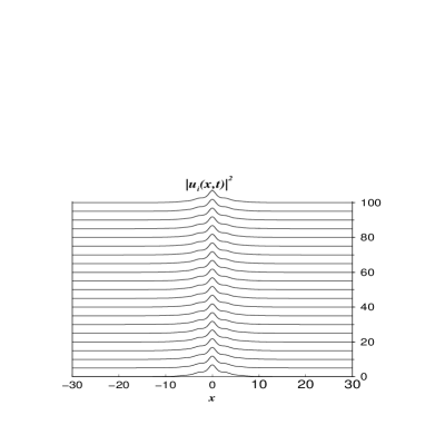
Figure 10: Top panel. Unstable OS mode of Townes soliton type (continuous curve) of Eq. (10) at the critical strength of the inter-species NOL $g_{1}=-1.3389$ for a delocalizing transition to occur. The mode has equal critical number of atoms $N_{1}=N_{2}=N_{c}=2$ with the same chemical potential $\mu_{1}=\mu_{2}=-0.03498$ and same profiles in both components. The dashed line represents the corresponding effective potential $V^{eff}_{1}=V^{eff}_{2}$ in Eqs. (53) and (54). Other parameters are fixed as $\gamma_{10}=-1,\gamma_{20}=-1$, $\gamma_{1}=\gamma_{2}=-0.5$, $g_{0}=1$. Bottom panel. Time evolution of the Townes soliton mode in the top panel as obtained from Eq. (10).

When $\gamma_{i0}=-g_{0}$, we obtain a system of coupled quintic NLS equations. For the symmetric case $U_{1}=U_{2}=U$, the system reduces to the quintic NLS equation

$$iU_{t}+U_{xx}+\chi|U|^{4}U=0,$$ (48)

with

$$\chi=\frac{3}{8}\gamma_{1}(\gamma_{1}+g_{1})+\frac{g_{1}}{8}(\gamma_{1}+3g_{1}+2\gamma_{2}).$$ (49)

The Townes soliton solution of Eq. (48) is

$$U(\mu,x)=e^{i\mu t}(\frac{3\mu}{\chi})^{1/4}\frac{1}{\cosh^{1/2}(2\sqrt{\mu}x)}.$$ (50)

with norm given by

$$N_{c}=\int_{-\infty}^{\infty}|U|^{2}dx=\frac{\pi}{2}\sqrt{\frac{3}{\chi}}.$$ (51)

This solution behaves as a separatrix between collapsing and decaying solutions of the quintic NLSE. Here $dN/d\mu=0$ and the VK criterion gives marginal stability. The total Hamiltonian is equal zero on this solution $H(U_{T})=0$. For example, for parameters values $g_{0}=-1,g_{1}=-1.3389,\gamma_{1}=\gamma_{2}=-0.5$, we obtain the critical number $N_{c}=2.41$. A comparison with the numerical results in Fig. 10 shows that the averaged NLS quintic equation overestimates the critical number $N_{c}$ by about $20$ percent(notice that for the same parameters values we have $N_{c}=2$ in Fig. 10). From this we conclude that the quintic NLS can be used only as a qualitative model for the delocalizing transitions of two component BEC in NOL. In the following we shall investigate Townes solitons and delocalizing transitions by recurring to numerical methods. Delocalizing transitions in binary BEC mixtures with NOL and in coupled NLS equations with cubic-quintic nonlinearities have not been previously investigated.

To show the existence of this phenomenon in a binary BEC mixture in a NOL we vary in time the parameter $g_{1}$ characterizing the intra-species interaction while keeping fixed the inter-species NOLs to which the two component are subjected. Starting from a given value of ${g_{1}}_{0}$, for which a stable OS-OS mode exists, we adiabatically decrease $g_{1}$ to a value ${g_{1}}_{0}-\Delta g_{1}$ and then increase it back to the original value.

In absence of delocalizing transitions the state will restore to its original form for any decrement $\Delta g_{1}$, while in presence of a delocalizing transition a threshold value for $\Delta g_{1}$ will appear above which the state becomes irreversibly delocalized (it cannot be restored to its original form). In Fig. 11 we show the time evolution of an OS-OS symmetric state with an equal number of atoms in the two components, during a variation of the inter-species interaction in time according of the form

$$g_{1}(t)={g_{1}}_{0}\{1-\Delta g_{1}\cos[\pi\frac{t-\frac{1}{2}(t_{1}+t_{2})}{t_{2}-t_{1}}]\}.$$ (52)

Figure 11: Delocalizing transition of an OS-OS mode of a binary BEC mixture with equal number of atoms $N_{1}=2,N_{2}=2$. The top panel shows the time evolution of the mode when the inter-species parameter $g_{1}$ is varied according to Eq. (52) with $t_{1}=50$, $t_{2}=150$, $\Delta g_{1}=0.25$. The bottom panel shows the same evolution but for the case $\Delta g_{1}=0.34$. Other parameters are fixed as $\gamma_{10}=-1,\gamma_{20}=-1$, $\gamma_{1}=\gamma_{2}=-0.5$, $g_{0}=1$, ${g_{1}}_{0}=-1.5$. The chemical potentials of the initial states at $t=0$ are $\mu_{1}=\mu_{2}=-0.5401$.

From the top panel of this figure it is clear that for a small decrement $\Delta g_{1}$ the state is able to restore the initial waveform, while for a larger decrement the state becomes fully delocalized. In analogy to what has been done for the NLS equation with periodic potential and quintic nonlinearity AS05 , one can characterize the delocalizing transition in terms of the unstable states which separate localized modes from extended ones. For the parameter used in Fig. 11, the critical value in the strength of the NOL for the occurrence of a delocalizing transition is found to be $N_{c}=2$. In Fig. 10 we show the existence of an unstable stationary state found in correspondence of this value, which has properties similar to the Townes solitons of the quintic 1D NLS or of cubic multidimensional NLS. Note that this stationary state corresponds to the unstable branch presented in the bottom panel of Fig. 4 [see the exact results for $x_{0}=0$].

From Fig. 12, it is indeed clear that for slight undercritical variations of the norm (number of atoms) the state becomes delocalized, while for slight overcritical variations of the norm it shrinks to a fully localized mode, resembling the behavior of Townes solitons. Notice that due to the equal number of atoms $N_{1}=N_{2}$ the modes in the two components have identical chemical potentials and identical profiles.

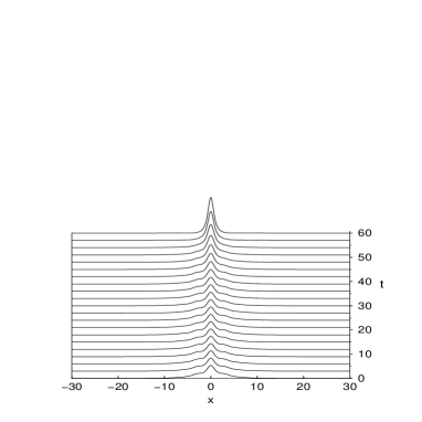
Figure 12: Time evolution of the Townes soliton mode in Fig. 10 for an undercritical $N_{und}=(.999)^{2}N_{c}$ (top panel) and overcritical $N_{ov}=(1.001)^{2}N_{c}$ (bottom panel) number of atoms. Other parameters are fixed as in Fig. 10.

A delocalizing transition is also observed for OS-OS states with different number of atoms in the two components. In this case the system shows a much rich behavior due to the possibility to use the inter-species interaction to stabilize localized states which in absence of interaction would be extended over the whole system. An example of such inter-species induced localization is given in Fig. 14 for an OS-OS symmetric states of Fig. 13 with an unbalanced number of atoms (a large difference in the number of atoms in the two components). In particular, in absence of the inter-species interactions, the first component has enough atoms to be above the delocalizing threshold, while the second component is taken to be below such a threshold, so that the state delocalizes in absence of interaction. From Fig. 14 we see, indeed, that the presence of the inter-species interaction prevents the second component to delocalize, while in absence of the inter-species interaction the first component remains localized and the second one delocalizes in a quite short time. Due to the many parameters of the problem, a full investigation of the delocalizing transitions of the fundamental OS-OS mode in binary BEC mixtures with NOL requires more extensive numerical investigations. We plan to do this in a separated publication.

Figure 13: Onsite symmetric mode of Eq. (10) with unbalanced number of atoms $N_{1}=2,N_{2}=0.5$, and for NOL parameters: $\gamma_{10}=-1,\gamma_{20}=-1$, $\gamma_{1}=\gamma_{2}=-0.5$, $g_{0}=-1$, $g_{1}=-1.5$. The continuous (dashed) curve refer to the first (second) component. The chemical potentials of the modes are $\mu_{1}=-1.013,\mu_{2}=-1.412.$ The dashed line refers to the second component.

Figure 14: Time evolution of the OS-OS mode in Fig. 13 in the presence (top panels) and in the absence (bottom panels) of the inter-species NOL of strength $g_{0}=-1,g_{1}=-1.5$.

V Conclusion

In this paper we have investigated the localized states in two-component BEC with periodic modulation in space intra-species and inter-species scattering lengths. The stability regions are analyzed using the variational approach and the Vakhitov-Kolokolov criterion. The symmetry properties (with respect to the NOL) of the localized modes in each component were considered and their stability properties investigated. We showed that localized modes of OS-OS type are always stable and represents the fundamental ground states of the system in the presence of attractive interactions. Intersite symmetric modes and mixed symmetry modes also exist but they appear to be metastable under GPE time evolution, decaying into modes of OS-OS-type. The existence regions in the parameter space of strongly localized modes (localized on few cells of the NOL) of fundamental type were predicted by mean of the variational ansatz and their stability properties predicted by the Vakhitov-Kolokolov criterion. Localized modes on tops of periodic backgrounds and of bright-dark solitons were also shown to exist in the case of binary mixtures with opposite interactions in the two components.

In spite of the quasi 1D nature of the problem we showed that fundamental solitons undergo a delocalizing transition when the strength of the intersite non linear optical lattice is varied. This transition was associated with the existence of an unstable localized solution which extends on many lattice cells of the the NOL and which exhibit a shrinking (decaying) behavior for slightly overcritical (undercritical) variations in the number of atoms.

This behavior was shown to exists for fundamental modes both with equal and unequal numbers of atoms in the two components.

The existence of the delocalizing transition for the fundamental modes was inferred also from a reduced vector GPE obtained by averaging the original GPE system with respect to the rapid spatial oscillations introduced by the NOL. The process of averaging the NOL introduces high order nonlinearities (cubic-quintic) which make the problem to be effectively equivalent to an higher dimensional vector GPE system for which delocalizing transition, in analogy to single component multidimensional cases, are usually expected.

The study of the delocalizing transition for fundamental multi-component solitons in terms of an averaged vector GPE with higher order nonlinearities, as well as the extension of the above analysis to the multidimensional case, appear to be interesting problems which deserve further investigations.

Appendix - Numerical Approach

The numerical methods employed in this paper are described in the following subsections.

V.1 Self-consistent diagonalization algorithm

We solve the nonlinear eigenvalue problem in (10) by treating the nonlinear part in self consistent manner. This amounts to consider the following linear eigenvalue problem

$$\mu_{1}u_{1}=-\frac{\partial^{2}u_{1}}{\partial x^{2}} + V^{eff}_{1}u_{1},$$ (53)

$$\mu_{2}u_{2}=-\frac{\partial^{2}u_{2}}{\partial x^{2}} + V^{eff}_{2}u_{2},$$ (54)

with the effective potentials defined as $V^{eff}_{i}=\gamma_{i}(x)|u_{i}|^{2}+g(x)|u_{3-i}|^{2}$, $\;i=1,2$. To solve these eigenvalue problem we adopt a discrete variable representation harris and diagonalize the operators $\hat{H}_{i}=\hat{K}+\hat{V}^{eff}_{i}$ in the discrete coordinate space representation $\{x_{n}=na\}$, $n=1,...,N_{p}$, $a=L/N_{p}$. Here $\hat{K}$ denotes the kinetic energy operator $\hat{K}=-\frac{\partial^{2}}{\partial x^{2}}$, $L$ is the length of the system and $N_{p}$ the number of grid points. By taking as a basis the set of vectors $|x_{n}>=(0,...0,1,0,...0)$, $n=1,...,N_{p}$ and noting that $V^{eff}_{i}$ is already diagonal in this basis while $\hat{K}$ is diagonal in the momentum representation $\langle k_{n}|\hat{K}|k_{m}\rangle=k_{n}^{2}\delta_{n,m}$, we have that the matrix elements of $\hat{H}_{i}$ can written as

$$\langle x_{n}|\hat{H}_{i}|x_{m}\rangle=\langle x_{n}|\hat{F}^{-1}\hat{K}\hat{F}|x_{m}\rangle+V^{eff}_{i}(na)\delta_{n,m},$$ (55)

where $\hat{F}|x_{n}\rangle$ denotes the Fourier (unitary) transform of the vector $|x_{n}\rangle$. Standard diagonalization routines are then used to find eigenvalues (chemical potentials) and eigenfunctions. The nonlinear eigenvalue is then solved in self-consistent manner starting from trial wavefunctions $u_{1}$, $u_{2}$, calculating the effective potentials , solving the eigenvalue problems (53) by diagonalizing the correspondig matrices (55), selecting given eigenstates as new trial functions, and iterating the procedure until convergence is reached (see Refs.LP05 ; Cruz07 for applications to single and multicomponent BEC cases).

V.2 Relaxation technique

The method of relaxation technique was used to check the results obtained with the previous method, to improve their accuracy, and also to make a complete study on the stability of the solutions.

Stable states are obtained using standard relaxation algorithm in imaginary time propagation, fixing the normalizations given by number of atoms of the two species, $N_{1}$ and $N_{2}$, and obtaining the chemical potentials $\mu_{1}$ and $\mu_{2}$. For the hyperbolic (unstable) states we extended to a coupled equation system the method developed in Ref.marijana , scheme C, in which the idea of “back renormalization” was used. In this method, it is given the chemical potential to obtain the number of atoms.

For a coupled system, the scheme C of Ref. marijana can be generalized, evolving the following equations in imaginary time:‘

$$-\frac{\partial\varphi}{\partial\tau} = \left(-\frac{\partial^{2}}{\partial x^{2}}+N_{1}\beta_{1}|\varphi|^{2}+N_{2}\sigma_{12}|\phi|^{2}-\mu_{1}\right)\varphi$$ (56)

$$-\frac{\partial\phi}{\partial\tau} = \left(-\frac{\partial^{2}}{\partial x^{2}}+N_{2}\beta_{2}|\phi|^{2}+N_{1}\sigma_{12}|\varphi|^{2}-\mu_{2}\right)\phi,$$ (57)

where we have normalized $\varphi$ and $\phi$ to one, such that $\varphi\equiv u_{1}/\sqrt{N_{1}}$ and $\phi\equiv u_{2}/\sqrt{N_{2}}$. $\beta_{i}$ and $\sigma_{12}$ are given by Eq. (5).

In discretized version, the coupled equations (56) and (57) takes the form

$$\varphi^{n+1/3} \leftarrow \varphi^{n}+\frac{\Delta\tau}{2}\left(\mu_{1}-\beta_{1}N_{1}^{n}|\varphi^{n}|^{2}-\sigma_{12}N_{2}^{n}|\phi^{n}|^{2}\right)\varphi^{n}$$

$$\varphi^{n+2/3} \leftarrow O_{CN}\varphi^{n+1/3}$$

$$\varphi^{n+1} \leftarrow \varphi^{n+2/3}+\frac{\Delta\tau}{2}\left(\mu_{1}-\beta_{1}N_{1}^{n}|\varphi^{n}|^{2}-\sigma_{12}N_{2}^{n}|\phi^{n}|^{2}\right)\varphi^{n}$$

$$\phi^{n+1/3} \leftarrow \phi^{n}+\frac{\Delta\tau}{2}\left(\mu_{2}-\beta_{2}N_{2}^{n}|\phi^{n}|^{2}-\sigma_{12}N_{1}^{n}|\varphi^{n}|^{2}\right)\phi^{n}$$

$$\varphi^{n+2/3} \leftarrow O_{CN}\varphi^{n+1/3}$$

$$\phi^{n+2/3} \leftarrow \phi^{n+2/3}+\frac{\Delta\tau}{2}\left(\mu_{2}-\beta_{2}N_{2}^{n}|\phi^{n}|^{2}-\sigma_{12}N_{1}^{n}|\varphi^{n}|^{2}\right)\phi^{n}$$

$$N_{1}^{n+1} \leftarrow \frac{N_{1}^{n}}{\displaystyle\int dx|\phi^{n+1}|^{2}},$$

$$N_{2}^{n+1} \leftarrow \frac{N_{2}^{n}}{\displaystyle\int dx|\varphi^{n+1}|^{2}},$$

$$\varphi^{n+1} \leftarrow \frac{\varphi^{n+1}}{\displaystyle\int dx|\varphi^{n+1}|^{2}},$$

$$\phi^{n+1} \leftarrow \frac{\phi^{n+1}}{\displaystyle\int dx|\phi^{n+1}|^{2}},$$

where the superscripts ($n$, $n+1$, etc) refer to time steps. $O_{CN}$ is the Crank-Nicolson evolution operation corresponding to $-{\partial^{2}}/{\partial x^{2}}$. Note that, in this coupled system the back renormalization (of $N_{1}^{n+1}$ and $N_{2}^{n+1}$) is done by exchanging the corresponding wavefunctions (as $N_{1}$ is associated to $\varphi$ and $N_{2}$ to $\phi$). This procedure is required for stability, as verified in numerical tests.

The excited states IS-OS and IS-IS depicted in Fig. 6 can be obtained by relaxing Eqs. (56)-(57) for $x\geq 0$ and imposing the Von Neumann boundary conditions in the origin, i.e., at $x=0$, $\partial\varphi/dx=0$ and $\partial\phi/\partial x=0$. The present relaxation algorithms are unable to find the state shown in Fig. 8, which was obtained by the approach given in subsection A.

As compared to the scheme shown in subsection A, the advantage of relaxation methods relies on the possibility of generalization to higher dimensions with few computational resources.

References

- (1) O. Morsh and M. Oberthaler, Rev. Mod. Phys. 78, 179 (2006).
- (2) V.A. Brazhnyi and V.V. Konotop, Mod. Phys. Lett. B 18, 627 (2004).
- (3) V.V. Konotop and M. Salerno, Phys. Rev. A, 65, 021602 RC (2002).
- (4) A. Trombettoni and A. Smerzi, Phys. Rev. Lett. 86, 2353 (2001).
- (5) F.Kh. Abdullaev, B.B.Baizakov, S.A. Darmanyan, V.V. Konotop, and M. Salerno, Phys. Rev. A 64, 043606 (2001).
- (6) I. Carusotto, D. Embriaco, G.C. La Rocca, Phys. Rev. A 65, 53611 (2002).
- (7) B. Eiermann, Th. Anker, M. Albiez, M. Taglieber, P. Treutlein, K.-P. Marzlin, and M. K. Oberthaler, Phys.Rev.Lett. 92, 230401 (2004).
- (8) B.P. Anderson and M.A. Kasevich, Science 282, 1686 (1998).
- (9) M. Greiner, O. Mandel, T. Esslinger, T.W. Hansch and I. Bloch, Nature (London) 415, 39 (2002).
- (10) B.B. Baizakov, V.V. Konotop, and M. Salerno, J. Phys. B 35 5105 (2002); B.B. Baizakov, B.A. Malomed, and M. Salerno, Europhys. Lett. 63, 642 (2003); E.A. Ostrovskaya, Yu.S. Kivshar, Phys. Rev. Lett. 90, 160407 (2003).
- (11) S.Inouye et al. Nature(London) 392, 151 (1998); J. Stenger et al., Phys. Rev. Lett. 82, 2422 (1999); J.L. Roberts et al., Phys. Rev. Lett. 81, 5109 (1998); S.L. Cornish, N.R. Claussen, J.L. Roberts, E.A. Cornell, and C.E. Wieman, Phys. Rev. Lett. 85, 1795 (2000); E.A. Donley et al., Nature(London) 412, 295 (2001).
- (12) F.Kh. Abdullaev and M. Salerno, J.Phys. B 36, 2851 (2003).
- (13) G. Theocharis, P. Schmelcher, P.G. Kevrekidis, and D.J. Frantzeskakis, Phys. Rev. A 72, 033614 (2005).
- (14) F.Kh. Abdullaev, A. Gammal, A.M. Kamchatnov, and L. Tomio, Int.J. Mod.Phys. B 19, 3415 (2005).
- (15) J. Garnier and F.Kh. Abdullaev, Phys. Rev. A 74, 013604 (2006).
- (16) P. Niarchou, G. Theocharis, P.G. Kevrekidis, P. Schmelcher, and D.J. Frantzeskakis, Phys. Rev. A 76, 023615 (2007).
- (17) H. Sakaguchi and B.A. Malomed, Phys. Rev. E 72, 046610 (2005); Phys.Rev. E 73, 026601 (2006).
- (18) F.Kh. Abdullaev and J. Garnier, Phys. Rev. A 72, 061605(R) (2005).
- (19) P.O. Fedichev, Yu. Kagan, G.V. Shlyapnikov, and J.T.M. Walraven, Phys. Rev. Lett. 77, 2913 (1996).
- (20) Y.V. Bludov and V.V. Konotop, Phys. Rev. A 74, 043616 (2006).
- (21) F.Kh. Abdullaev, A.A. Abdumalikov, and R.M. Galimzyanov, Phys. Lett. A 367, 149 (2007).
- (22) Y. Sivan, G. Fibich, and M.I. Weinstein, Physica D 217, 31 (2006); Phys. Rev. Lett. 97, 193902 (2006).
- (23) J. Belmonte-Beitia, V.M. Perez-Garcia, V. Vekslerchik, P.J. Torres, Phys. Rev. Lett. 98, 064102 (2007).
- (24) G. Dong and B. Hu, Phys. Rev. A 75, 013625 (2007).
- (25) Yu.V. Bludov, V.A.Brazhnyi, and V.V. Konotop, Phys. Rev. A 76, 023603 (2007).
- (26) B.B. Baizakov and M. Salerno, Phys. Rev. A 69, 013602 (2004).
- (27) M. Salerno, Laser Physics, 15, 620 (2005).
- (28) M. Brtka, A. Gammal, and L. Tomio, Phys. Lett. A 359, 339 (2006).
- (29) A. Simoni, F. Ferlaino, G. Roati, G. Modungo, and M. Inguscio, Phys. Rev. Lett. 90, 163202 (2003).
- (30) K. Kasamatsu and M. Tsubota, Phys. Rev. Lett. 93, 100402 (2004).
- (31) P.G. Kevrekidis, H. Susanto, R. Carretero-Gonzalez, B.A. Malomed, and D.J. Frantzeskakis, Phys. Rev. E 72, 066604 (2005).
- (32) H.J. Miesner et al., Phys. Rev. Lett. 82, 2228 (1999).
- (33) H. Gimperlein, S. Wessel, J. Schmiedmayer, and L. Santos, Phys. Rev. Lett. 95, 170401 (2005).
- (34) M. Theis, G. Thalhammaer, K. Winkler, M. Hellwig, G. Ruff, R. Grimm, and J.H. Denschlag, Phys. Rev. Lett. 93, 123001 (2004).
- (35) N.G. Vakhitov and A.A. Kolokolov, Radiophysics and Quantum Electronics 16, 783 (1973).
- (36) H. A. Cruz, V. A. Brazhnyi, V. V. Konotop, G. L. Alfimov, and M. Salerno, Phys. Rev. A 76, 013603 (2007).
- (37) F.Kh. Abdullaev and M. Salerno, Phys. Rev. A 72, 033617 (2005).
- (38) D.O. Harris et al., J. Chem. Phys. 43 1515 (1965).