X-ray Fluorescent Fe K$\alpha$ Lines from Stellar Photospheres

Abstract

X-ray spectra from stellar coronae are reprocessed by the underlying photosphere through scattering and photoionization events. While reprocessed X-ray spectra reaching a distant observer are at a flux level of only a few percent of that of the corona itself, characteristic lines formed by inner shell photoionization of some abundant elements can be significantly stronger. The emergent photospheric spectra are sensitive to the distance and location of the fluorescing radiation and can provide diagnostics of coronal geometry and abundance. Here we present Monte Carlo simulations of the photospheric K$\alpha_{1},\alpha_{2}$ doublet arising from quasi-neutral Fe irradiated by a coronal X-ray source. Fluorescent line strengths have been computed as a function of the height of the radiation source, the temperature of the ionising X-ray spectrum, and the viewing angle. We also illustrate how the fluorescence efficiencies scale with the photospheric metallicity and the Fe abundance. Based on the results we make three comments: (1) fluorescent Fe lines seen from pre-main sequence stars mostly suggest flared disk geometries and/or super-solar disk Fe abundances; (2) the extreme $\approx 1400$ mÅ line observed from a flare on V 1486 Ori can be explained entirely by X-ray fluorescence if the flare itself were partially eclipsed by the limb of the star; and (3) the fluorescent Fe line detected by Swift during a large flare on II Peg is consistent with X-ray excitation and does not require a collisional ionisation contribution. There is no convincing evidence supporting the energetically challenging explanation of electron impact excitation for observed stellar Fe K$\alpha$ lines.

1 Introduction

It is well-established from surveys of the sky at EUV and X-ray wavelengths that all stars with spectral types later than mid-F, except for giants later than mid-K, possess hot outer atmospheres akin to that of the Sun (e.g. Vaiana et al., 1981; Schmitt, 1997). While much observational and theoretical effort has been devoted to understanding solar coronal spectra and, in more recent years, toward understanding stellar coronal emission and spectra, comparatively little attention has been devoted to the reprocessing and line fluorescence resulting from this coronal emission by the underlying solar and stellar photospheres. In contrast, considerable effort has been spent on the study of X-ray reprocessing by “cold” gas in much more complex systems with more prominent fluorescent features but more uncertain geometries and physical conditions, such as the accretion disks around black holes and non-degenerate objects in X-ray binaries (e.g. Felsteiner & Opher, 1976; Hatchett & Weaver, 1977; Fabian et al., 1989; George & Fabian, 1991; Laor, 1991; Matt et al., 1997; Ballantyne et al., 2002; Beckwith & Done, 2004; Čadež & Calvani, 2005; Dovčiak et al., 2004; Laming & Titarchuk, 2004; Brenneman & Reynolds, 2006). The processes involved in photospheric fluorescence by coronal irradiation are the same as those discussed in these works; the main difference here is in the specific geometry of the X-ray source above a quasi-neutral sphere and of the extended, shell-like nature of the coronal source above the photosphere during quiescent conditions.

X-rays emitted from a hot ($T\gtrsim 10^{6}$ K) corona incident on the underlying photosphere can undergo either Compton scattering or photoabsorption events through the ionization of atoms or weakly ionized species. Through scattering events, photons can be reflected back in a direction towards the stellar surface where they have a finite chance of escape. Compton scattering redistributes the spectrum to lower energies by $\sim E^{2}/m_{e}c^{2}$ per collision, where $E$ is the photon energy and $m_{e}$ the electron rest mass. The spectrum reflected from a stellar surface by scattering events is then shifted and broadened towards lower energies. Photoionization events involving X-ray photons directed toward the photosphere are predominantly inner shell interactions with astrophysically abundant elements, the outer and valance cross-sections being very small at these energies. Observable fluorescent lines can then arise as a result of the finite escape probabilities of photons emitted in outward directions by hole transitions in these atoms photoionized in their inner shells. These processes have been described in the solar context by, e.g., Tomblin (1972) and Bai (1979) (B79), and more recently for arbitrarily photoionized slabs by Kallman et al. (2004).

The strongest of the fluorescent lines for a plasma of approximately cosmic composition is the $2s$-$1p$ 6.4 keV Fe K$\alpha$ doublet occurring following ejection of a $1s$ electron. It has been observed in solar spectra on numerous occasions (e.g. Neupert et al., 1967; Doschek et al., 1971; Feldman et al., 1980; Tanaka et al., 1984; Parmar et al., 1984; Zarro et al., 1992). The mechanism of fluorescence by the thermal X-ray coronal continuum was suggested by Neupert et al. (1967), and was firmly established on more theoretical grounds by Basko (1978, 1979) and B79. Parmar et al. (1984) provided convincing observational confirmation based on flare spectra obtained by the Solar Maximum Mission, though it has also been noted that contributions from non-thermal electron impact might also be present during hard X-ray bursts (e.g. Emslie, Phillips, & Dennis, 1986; Zarro, Dennis, & Slater, 1992).

B79 pointed out that, for a given source spectrum, the observed flux of Fe K$\alpha$ photons from the photosphere depends on essentially three parameters: the photospheric iron abundance; the height of the emitting source; and the heliocentric angle between the emitting source and observer. Phillips et al. (1994) used Fe K$\beta$ observations to probe the difference between the photospheric and coronal iron abundance for flares observed by the Yohkoh satellite. More importantly for the stellar case, the spatial aspects of photospheric fluorescent line formation suggest its application to understanding the spatial distribution of coronal structures and flares on stars of different spectral type and activity level to the Sun (Drake et al., 1999). Indeed, Fe K fluorescence has recently been detected during flares on the active binary II Peg (Osten et al., 2007) and on the single giant HR 9024 (Testa et al., 2007). The Fe K line has also been seen in a growing sample of pre-main sequence (PMS) stars (Imanishi et al., 2001; Favata et al., 2005; Tsujimoto et al., 2005; Giardino et al., 2007), in which the line is thought to originate predominantly from the irradiated protoplanetary disk rather than the photosphere.

Since the work of Bai (1979), there have been no concerted efforts to extend models of photospheric fluorescence for coronal excitation sources with other characteristics. Fluorescent lines other than Fe K$\alpha$ have also not yet, to our knowledge, been studied by other workers in any detail in this context. A reasonably strong feature observed in solar spectra near 17.62 Å had been identified with Fe L$\alpha$ photospheric fluorescence (McKenzie et al., 1980; Phillips et al., 1982), but calculations of the expected line strength was shown by Drake et al. (1999) to be much too weak to explain the feature, and these authors instead identified the line with a transition in Fe XVIII arising from configurational mixing and both seen in Electron Beam Ion Trap spectra and predicted by theory (Cornille et al., 1992). However, given the potential diagnostic value of photospheric fluorescence, other lines, such as O K$\alpha$, are possibly observable with very high quality observations and warrant further study.

The capabilities of current X-ray missions such as Chandra, XMM-Newton, Swift and Suzaku to detect fluorescent lines further motivates a re-examination of the photospheric fluorescence problem in the context of stellar coronae, photospheres and protoplanetary disks. We restrict the study in hand to Fe K fluorescence from stellar photospheres and defer detailed discussions of protoplanetary disks and fluorescence from other elements to future work.

2 Calculations of Photospheric Fluorescent Spectra

2.1 Photospheric Penetration of Coronal X-rays

In order to establish the atmospheric conditions under which fluorescence by, and Compton scattering of, coronal X-rays take place, it is necessary to know where in a stellar atmosphere incident X-rays are absorbed. Since the absorption cross-section for a cool plasma with solar, or near-solar, composition is a strong function of photon energy, the absorption of the coronal X-ray spectrum will take place at different levels in the atmosphere. To determine the characteristic height of absorption as a function of photon energy we have computed the optical depth for X-rays as a function of altitude in the solar atmosphere. We adopted the Vernazza, Avrett, & Loeser (1981) Model C (VALC) describing the solar atmospheric structure as a function of altitude, and used the photoionization cross-sections from Verner et al. (1993) and Verner & Yakovlev (1995) to compute the optical depth. The total absorption cross-section for a plasma with the solar chemical composition of Grevesse & Sauval (1998) (GS) in the energy range of interest for this study is illustrated in Figure 1 for the case of both a neutral gas and a plasma in which all species are once-ionized (this latter situation does not correspond to any physically valid thermal equilibrium condition, but is simply for comparative purposes).

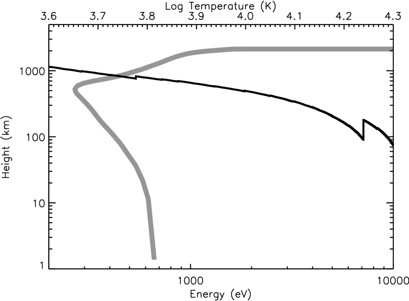
Figure 2: The locus corresponding to optical depth of unity for X-rays incident on the solar photospheric VALC model plotted as a function of incident photon energy and height (thin black curve). Toward lower energies absorption occurs predominantly in the lower chromosphere; this region is shifted downwards with increasing energy, reaching the upper photosphere at the Fe K photoionization threshold energy. The model temperature structure as a function of height is illustrated by the thick grey curve.

The height in the VALC model corresponding to optical depth of unity for X-rays is illustrated in Figure 2. Also illustrated is the atmospheric temperature as a function of height in this figure for comparison purposes. At the energy corresponding to the absorption edge of C, optical depth of unity is reached in the lower chromosphere, at temperatures of $\sim 6000$ K and about 1000 km above the point where the continuum optical depth at 5000 Å, $\tau_{5000}$, is unity (defined to be at a height of 0 km in this model). Towards higher energies, the decreasing photoabsorption cross-section leads to increasingly deeper penetration of coronal X-rays. At the Fe K photoionization threshold energy, the typical height of absorption is well into the photosphere and only 100 km or so above $\tau_{5000}=1$. At this point in the solar atmosphere, most Fe is in the form of Fe⁺ and the temperature is $\sim 5400$ K.

Number densities in this region of the VALC model range from n$>10^{16}$ down to $10^{13}$ cm^-3 and decrease roughly exponentially with an scale height $\sim 130$ km. Thus the ionization parameter, $U\sim F/n$ (e.g. Davidson & Netzer, 1979), where $F$ is the ionizing photon flux per unit area, is small for even the strongest flares and X-ray photoionization of the photospheric gas is inconsequential. This is in contrast to models of, e.g., X-ray irradiated accretion disks where the ionization state of the reflecting medium is governed by the incident hard photon flux and must be computed self-consistently with the emergent X-ray spectrum (e.g. Kallman et al., 2004).

The range of heights in the photosphere where the X-ray photons are absorbed is very small compared with the stellar radius (of order $\sim 100$-$1000$ km), and the variation in temperature and ionization is also small over this altitude range (Figure 2). We therefore approximate the photosphere by a geometrically thin but optically very thick shell of homogeneous density. We set the density to an arbitrarily high value such as to obtain the same behaviour as for a plane-parallel model where the photosphere is approximated by a cold semi-infinite slab with constant density. The appropriate atmospheric reference frame for describing the absorption, scattering and fluorescent processes is the mass or particle column depth and the calculations are independent of the absolute value of the density. Provided plane-parallel geometry remains a good approximation, these calculations should therefore be valid for stars with different surface gravities and atmospheric pressures.

By assuming the photosphere to be cold, we make no distinction between fluorescence processes in species of different charge states. In typical late-type stellar photospheres the dominant species are neutral and once-ionized, for which the splitting between the respective fluorescence lines is very small as are differences in fluorescent yields (House, 1969; Kallman et al., 2004). We also note that, as illustrated in Figure 1, in the energy range of interest here there is essentially no difference in the photoabsorption cross-sections for neutral or once-ionized species except at low energies where the difference is dominated by He and H. In reality, it is only the metals with fairly low first ionization potentials that are significantly ionized in the upper photosphere and lower chromosphere while He and H are almost entirely neutral.

2.2 Monte Carlo (MC) Calculations of Fluorescent Processes

We use a modified version of the MC photoionization and radiative transfer code mocassin (Ercolano et al., 2003, 2005). This code uses a stochastic approach to the transfer of radiation which allows the construction of models of arbitrary geometry where all components of the radiation field are treated self-consistently. The basic idea is to employ a discrete description of the radiation field, whereby the simulation quanta are monochromatic packets of radiation of constant energy, $\varepsilon_{0}$, (Abbott & Lucy, 1985). The individual processes of scattering, absorption and re-emission of radiation can then be simulated by sampling probability density functions based on the medium opacities and emissivities, thus allowing the determination of the trajectories of packets as they leave the illuminating source(s) and diffuse outward. These trajectories constitute the MC observable of our experiment which can be related to the mean intensity of the radiation field via the following MC estimator (Lucy, 1999):

$$4\pi\,J_{\nu}\,d\nu\,=\,\frac{\varepsilon_{0}}{\Delta t}\frac{1}{V}\sum_{d\nu}l,$$ (1)

where $V$ is the volume of the current grid cell and the summation is over all the fragments of trajectory, $l$, in $V$, for packets with frequencies in the ($\nu$, $\nu+d\nu$) interval. $\Delta\,t$ is the duration of the Monte Carlo experiment. The significance of this estimator may be most easily understood by considering that the energy density of the radiation field in ($\nu$, $\nu+d\nu$) is $4\,\pi\,J_{\nu}\,d\nu/c$. At each given instant a packet contributes energy $\varepsilon_{0}$ to the volume element containing it. The time-averaged energy content of a volume element is given by the summation of the energy contribution of all packets crossing this volume element in the time interval $\Delta\,t$. Equation 1 follows from this argument, since each packet contributes $\varepsilon_{0}\,\delta\,t/\Delta\,t$ to the time averaged energy content of a volume element and $\delta\,t$ = $l/c$, where $l$ is the segment of the trajectory of a packet contained in the volume element.

mocassin’s atomic database is regularly updated and currently uses opacity data from Verner et al. (1993) and Verner & Yakovlev (1995), energy levels, collision strengths and transition probabilities from Version 5 of the CHIANTI database (Landi et al., 2006, and references therein) and the improved hydrogen and helium free-bound continuous emission data recently published by Ercolano & Storey (2006). The Verner & Yakovlev (1995) photoabsorption cross-sections do no not include the resonance structure that can be prominent near ionisation thresholds. While this structure can be important for some astrophysical applications (e.g. Kallman et al., 2004), it is not significant for the fluorescent efficiencies discussed here that depend primarily on broad-band spectral properties and neutral or once-ionised gas.

In the case of inner shell Fe K${\alpha}$ production, the fluorescent luminosity, L(Fe K${\alpha}$), due to the absorption of an incident energy packet of wavelength shorter than the Fe K edge ($h\nu~{}>~{}$ 7.11 keV) is calculated on the fly. The event of absorption of a high energy packet is immediately followed by the re-emission of a number, $n$ of Fe K${\alpha}$ packets from the same event location. For an incident packet of frequency $\nu$, carrying energy $\varepsilon_{0}$ in the unit time $\Delta\,t$, the total Fe K${\alpha}$ emission is given by

$$L(Fe\,K{\alpha})~{}=~{}nL^{\prime}(Fe\,K{\alpha})~{}=~{}n\,\frac{\varepsilon_{0}}{\Delta\,t}\frac{1}{h\nu}\,\frac{\sum_{i}\kappa_{\nu}^{Fe^{i}}Y_{Fe\,K{\alpha}}^{i}\varepsilon_{Fe\,K{\alpha}}^{i}}{\kappa_{\nu}^{gas}}R_{\alpha}$$ (2)

where $\kappa_{\nu}^{Fe^{i}}$ and $Y_{Fe\,K{\alpha}}^{i}$ are the absorption opacity and the Fe K${\alpha}$ yield of $i$-times ionised iron, $\varepsilon_{Fe\,K{\alpha}}^{i}$ is the energy of the K$\alpha$ line of i-times ionised iron ($\sim$6.4 keV) and the summation is over all abundant ionisation stages, $\kappa_{\nu}^{gas}$ is the absorption opacity due to all other abundant species and $R_{\alpha}$ is the branching ratio between $K{\alpha}$ and $K{\beta}$ fluorescence (0.882:0.118, Bambynek et al. 1972). We use a value of 0.34 for the fluorescence yields of neutral and once-ionised iron (Bambynek et al., 1972; Krause, 1979; Kallman et al., 2004).

The $n$ Fe K${\alpha}$ energy packets are emitted in random directions as the fluorescent emission process can be assumed to be isotropic. To ensure conservation, energy per unit time $(\varepsilon_{0}/\Delta\,t~{}-~{}L(Fe\,K{\alpha}))$ must also be immediately re-emitted from the event location, at a frequency determined by sampling the local emissivity of the medium and transferred through the grid as described by Ercolano et al. (2003).

The fates of the newly emitted Fe K${\alpha}$ packets are determined by the absorption and Compton opacities encountered along their diffusion paths. Fe K${\alpha}$ packets that are absorbed will be transformed into diffuse field packets or emission line packets at another energy and will not contribute to the emerging spectrum at 6.4 keV. Fe K${\alpha}$ packets that are Compton scattered will experience a change of direction and a shift in frequency (by approximately $(h\nu)^{2}$/$m_{e}c^{2}$), their new frequency and direction being determined using the Klein-Nishina formulae. These packets may therefore finally emerge and contribute to the low energy shoulder of the Fe K${\alpha}$ feature, or may undergo further scatterings and/or absorptions.

The emergent integrated and the direction-dependent spectral energy distributions (SEDs) are finally calculated using all escaped energy packets, including contributions from Compton reflected packets and fluorescence line packets. Our method also allows us to easily separate the various components of the emergent SED.

Since the study presented here is similar to the earlier B79 work, we summarise in brief the differences between these studies:

1. B79 was aimed at understanding Fe K$\alpha$ fluorescence in solar flares; the possible utility of fluorescence for estimating the photospheric Fe abundance (which was of course more uncertain that at present) was emphasised. The calculations presented here extend the parameter space so as to cover conditions found in large stellar flares and stars completely covered in X-ray emitting active regions; our emphasis is on the use of fluorescence as a diagnostic of coronal and flare geometry on distant unresolved stars.

2. Input parameters used here are more up-to-date in several respects. Input spectra have been computed using isothermal coronal plasma models whereas B79 used an analytical approximation to the bremsstrahlung continuum. B79 also adopted a simple form for absorption cross-sections of Fe and the photospheric gas. Here, photoabsorption cross-sections are computed self-consistently according to the chemical composition and ionisation state of the gas using analytical fits to Opacity Project data (Verner & Yakovlev, 1995). These abundance-weighted cross-sections are about 40% higher than that used by B79 for the gas with Fe excluded; the B79 cross-section for neutral Fe K-shell absorption is about 20% larger than that of Verner & Yakovlev (1995) at threshold, but very similar at energies above 8 keV. As we shall see below, these differences have little influence on the resulting fluorescence efficiencies, largely because the Fe cross-section dominates and differences here are small.

3. B79 assumed that once a Fe K$\alpha$ line photon is Compton scattered it is “lost” due to the shift in energy. Here, we follow all photons until they emerge from the photosphere and therefore also resolve the Compton shoulders comprising scattered line photons.

2.3 Benchmark Calculations of Iron K$\alpha$ in solar flares

In order to establish the robustness of our new code, we first examine the Fe K${\alpha}$ problem for point-like solar flares using the full 3D geometry of our models and fully self-consistent radiative transfer, treating photoabsorption contributions from all abundant atoms and ions, and (Compton) scattering by electrons. As a benchmark, we attempt to reproduce the earlier results of B79.

The photon density spectrum of the incident X-rays, $L(\varepsilon)$, is taken to follow the same bremsstrahlung power-law with energy, $\varepsilon$, as defined in B79:

$$L(\varepsilon)~{}=~{}A~{}\varepsilon^{-1}~{}\exp(-\varepsilon/kT)\;\rm photon~{}s^{-1}keV^{-1}$$ (3)

We consider four X-ray temperatures (0.5, 1.0, 3.0, 5.0 keV) and two flare heights, $h=0$ and $h=0.1~{}R_{\odot}$, which cover the full parameter space investigated by B79. In the remainder of this paper we will quote temperatures in degrees K, however in this section these are given in keV, which are the units used by B79. For the sake of comparison, we used the Fe abundance adopted by B79 of $n_{\rm Fe}$/$n_{\rm H}~{}=~{}4\times 10^{-5}$ by number; for other elements we adopted the mixture of GS. In Table 1 we compare our results for the iron K$\alpha$ fluorescence efficiency, $\Gamma$, to those of B79 (values in brackets). $\Gamma$ is defined as the ratio of the total luminosity of iron K$\alpha$ photons emitted from the photosphere and $N_{7.11}/2$, where $N_{7.11}=\int_{7.11}^{\infty}L(\varepsilon)\,dE$, with $L(\varepsilon)$ given by Equation 3.

In this formulation the flux of Fe K${\alpha}$ photons received at Earth is equal to

$$F_{K\alpha}=\frac{\Gamma f(\theta)N_{7.11}}{4\pi\,D^{2}},$$ (4)

where D is the distance from the source and $\theta$ the heliocentric angle subtended by the flare and observer.

The agreement with the results of B79 is generally very good, and significantly better at higher X-ray temperatures; discrepancies amount to only 18% for X-ray temperatures of 0.5 keV. We attribute the bulk of the differences in fluorescent efficiencies to the use by B79 of slightly different absorption cross-sections and an analytical approximation for the gas opacities, while we calculate these self-consistently according to the elemental abundances considered in our models. The slight temperature dependence in the differences is most likely due to the different slopes of the B79 functional form and our calculations, which take into account all elements with Z$<$30.

Our 3D models allow us to obtain the spectral energy distribution emerging from arbitrary viewing angles. In Figure 3 we show the variation of $f(\theta)$ for ten heliocentric angles from $5^{\circ}$ to $95^{\circ}$ for two flare heights ($h=0$ and $h=0.1R_{\odot}$). These plots are directly comparable with the top-left and bottom-right panels of Figure 3 of B79 and show good agreement with his results.

Finally, in Figure 4 we show the variation of $\Gamma$ as a function of iron abundance. Again, our results are in good agreement with those of B79 (cf his Figure 4) and show that the relation of the Fe K${\alpha}$ fluorescence efficiency on the photospheric iron abundance is weaker than a proportional relation, as expected. We discuss the Fe dependence of the Fe K$\alpha$ flux in more detail in §3.4 below.

3 New Fe K${\alpha}$ Diagnostic Calculations

Having in the previous section established the robustness of our methods, we present the results from a new grid of model calculations designed to provide useful diagnostics for Fe K${\alpha}$ detections for a wider range of stellar environments. In particular, stellar coronae cover a much wider range of temperatures and Fe abundance than the solar case and investigation of fluorescence over a wider range of parameters will be necessary for correct interpretation of fluorescent lines from stars.

We investigate two geometrical configurations: (i) a single flare and (ii) an active corona that can be approximated by a spherical shell illuminating a photosphere from particular scale height $h$. While coronae are of course not expected to conform to a shell-like geometry, this case should approximate quite well the case in which a star is quasi-uniformly covered in active regions. Coronal fluorescing spectra were adopted from a grid of isothermal models computed using emissivities from the CHIANTI compilation of atomic data (Landi et al., 2006, and references therein), together with ion populations from Mazzotta et al. (1998), as implemented in the PINTofALE IDL software suit (Kashyap & Drake, 2000). We adopted the chemical composition of GS for all calculations except where noted. While there will be some contribution from transitions in He-like and H-like Ni and the higher Lyman series of He-like and H-like Fe to the ionising photon flux $N_{7.11}$, this is small compared with the integrated continuum contribution; consequently the metallicity sensitivity for the ionising spectrum is generally negligible for realistic ranges of metallicity.

3.1 A Single Flare Illuminating a Photosphere

In the case of a single flare illuminating a photosphere from a given height, the heliocentric angle, $\theta$, has a dramatic effect on the Fe K${\alpha}$ flux detected. The intrinsic Fe K${\alpha}$ efficiency, $\Gamma$, is, of course, independent of $\theta$, being a function of the fluorescing spectrum, the flare height and the relative iron abundance. Using GS solar abundances for all elements with $Z\,<\,30$ we show in Table 2 the Fe K${\alpha}$ efficiency, $\Gamma$, predicted for X-ray temperatures in the range $T=6.4$–8.0 keV and flare height in stellar radii in the range $h=0$–$5R_{*}$.

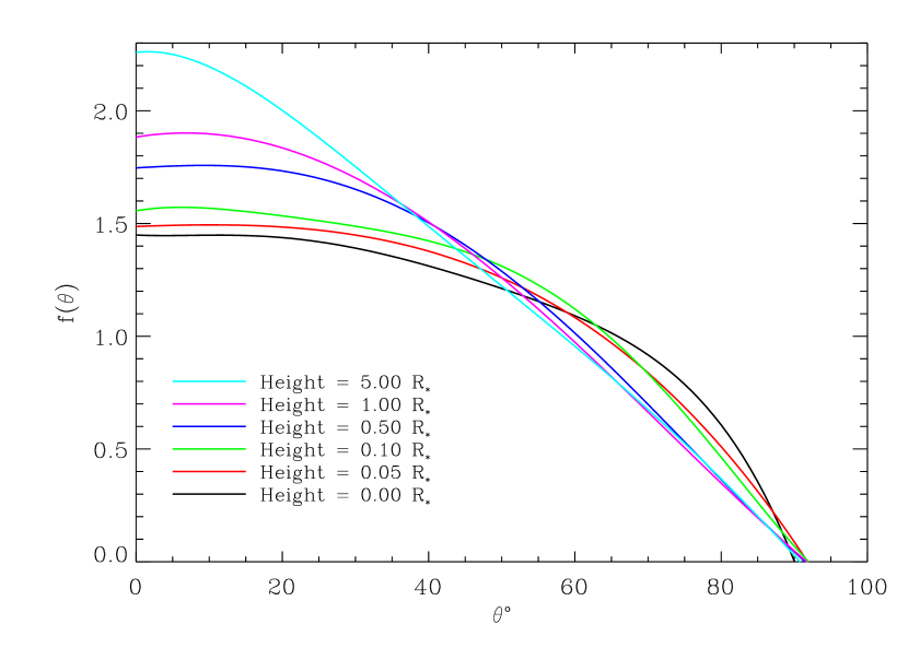
Figure 5: Fits to the $f(\theta)$ factor relating the Fe K${\alpha}$ fluorescence flux to the angle of observation obtained for six flare heights

In order to investigate the Fe K${\alpha}$ line strength as a function of heliocentric angle, we calculated $f(\theta)$ for a number of angles at each flare height. For convenience we fit our results using 4th or 5th order polynomials, such that $f(\theta^{o})~{}=~{}\sum_{i=0}^{5}\alpha_{i}\cdot\theta^{i}$. The fit coefficients are listed in Table 3 and the resulting $f(\theta)$ functions are plotted in Figure 5. Our fits are valid between heliocentric angles 0^∘ and 100^∘; the maximum errors between our data and the fits at each flare height are also listed as percentages in Table 3 and are less than 2.4%.

These functions illuminate interesting characteristics of the fluorescence problem for different incidence and exit angles. Firstly, we point out that for finite flare heights $h$, $f(\theta)$ is non-zero for angles $\theta>90^{\circ}$. This is simply due to the surface illumination from flares beyond the limb extending onto the visible hemisphere: the angle at which $f(\theta)$ reaches 0 is given geometrically by $\theta_{0}=90^{\circ}+arccos(R_{\star}/(R_{\star}+h))$. We note, however, that we did not explore the very low-response tail of $f(\theta)$ for heliocentric angles greater than $100^{\circ}$, as the Fe K$\alpha$ flux, although finite for some flare heights, is too small to be detectable even for very strong flares. Furthermore, $f(\theta)$ falls below the statistical variance of our models at these large angles.

The general decrease of $f(\theta)$ with increasing $\theta$ present in all curves is largely a result of the $1/cos(\theta)$ increase in path length required for K$\alpha$ photons to escape. The most conspicuous characteristic of $f(\theta)$ behaviour with different heights is the steepening of the decline from smaller to larger angles with increasing flare height. This arises because of the range of incidence angles of flare photons on the photosphere. As $h\rightarrow\infty$, incidence angles relative to the photospheric normal become smaller and the average penetration depth before interaction by either absorption or scattering events is larger. Consequently, path lengths increase and Fe K$\alpha$ escape probabilities decrease. Folded in with this is the decreasing fraction of photons incident on the visible hemisphere of the star with increasing $\theta$.

3.2 A Coronal Shell Illuminating a Photosphere

The calculations for $f(\theta)$ and $\Gamma$ can be readily adapted from the point source case to one in which the corona is approximated by a spherical shell of emission, as might be the case for stars significantly more active than the Sun. This can be seen by taking the shell case to be a large ensemble of point sources distributed uniformly about the star for which the observed fluorescent flux is then simply the solid angle average of the point source case,

$$F_{K\alpha}=\frac{\Gamma N_{7.11}}{4\pi D^{2}}\frac{1}{4\pi}\int f(\theta)\;d\Omega$$ (5)

Since, following from the definition of $\Gamma$ and our Equation 4, $\int f(\theta)\;d\Omega=2\pi$, the flux is

$$F_{K\alpha}=\frac{\Gamma N_{7.11}}{8\pi D^{2}}$$ (6)

By tailoring the solid angle integral in Equation 5 the fluorescent flux for an arbitrary coverage pattern of active regions viewed from any angle can be derived from the tabulated values of $f(\theta)$ and $\Gamma$.

3.3 Sensitivity to Ionising X-ray Temperature

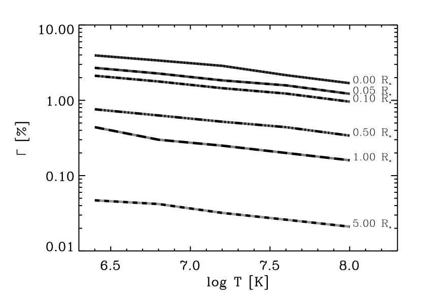
Figure 6: The fluorescence efficiency, $\Gamma$, as a function of the ionising X-ray spectrum temperature for different flare heights, computed for the GS solar abundance mixture.

The fluorescence efficiency, $\Gamma$, is illustrated as a function of the isothermal plasma temperature adopted for the ionising coronal spectrum in Figure 6. We find $\Gamma$ varies very slowly with temperature, decreasing by only a factor of $\sim 2$ over a factor of 30 or more in temperature. This gradual decrease is predominantly a result of the competition between Fe inner-shell absorption and Compton scattering. As temperatures increase, incident photons are present at higher and higher energies. Since the Fe cross-section declines with increasing photon energy while the Compton cross-section remains constant, higher energy photons are more liable to be scattered out of the photosphere before being destroyed by photoabsorption.

3.4 Sensitivity to Photospheric Fe Abundance and Metallicity

In the optically-thick fluorescence case such as characterizes the photospheric fluorescence problem, inner-shell photoabsorption by Fe atoms and ions competes with the background opacity from other elements. Observed Fe K$\alpha$ line fluxes and equivalent widths are then expected to vary predominantly according to the relative Fe abundance rather than just the photospheric metallicity. Note that the optically-thick situation differs to the optically-thin formalism discussed by Liedahl (1999) and referred to in the discussion of stellar and protostellar Fe K$\alpha$ lines (e.g. Favata et al., 2005; Tsujimoto et al., 2005; Osten et al., 2007): in the optically-thin case the fluorescent Fe line strength is primarily a function of the absorbing Fe column.

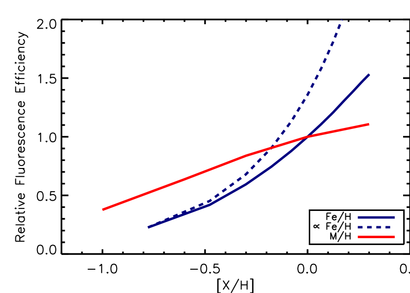
Figure 7: The fluorescence efficiency, $\Gamma$, as a function of logarithmic photospheric metallicity [M/H] and Fe abundance [Fe/H], normalised to its value for the solar mixture of GS. The efficiencies as a function of [Fe/H] were computed for GS values for the abundances of all other elements. The dashed curve represents the proportionality relation expected from scaling the efficiency linearly with Fe abundance from the lower Fe abundance point. Calculations where performed for an ionising X-ray spectrum with temperature of 10^7.2 K.

In extension to the benchmark calculations discussed in §2.3, we have computed the sensitivity of $F_{K\alpha}$ to the Fe abundance for a model fluorescing spectrum with a temperature of 10^7.2 K and Fe abundance in the range $-0.8\leq$[Fe/H]$\leq+0.3$ ($0.5\times 10^{-5}\leq n_{\rm Fe}/n_{\rm H}\leq 6\times 10^{-5}$). This temperature was chosen to be representative of a typical very active corona or moderate stellar flare. Trends with [Fe/H] are expected to be only weakly sensitive to this adopted temperature, the fluorescence efficiency, $\Gamma$, varying only very slowly with $T$ (Figure 6). The results are illustrated in Figure 7 where we show $\Gamma$ normalised to its value at the GS solar Fe abundance in comparison to the proportional relation, analogous to Figure 4 discussed in §2.3 and Figure 4 of B79.

The fluorescence line strength vs Fe abundance was investigated in the context of accretion disks by Matt et al. (1997), and our results are comparable to Figures 1 and 2 from that work for the range of Fe abundance in common. As noted above, B79 showed that the relationship between the relative fluorescence efficiency $\Gamma$ and the Fe abundances is weaker than a proportional relation. In fact, the relation increasingly departs from proportionality with increasing Fe abundance. This behaviour arises because of the equipartition of photoabsorption between the different species present in the atmosphere. At low Fe abundance when the background cross-section due to elements other than Fe dominate, $F_{K\alpha}$ varies according to $n_{\rm Fe}\sigma_{\rm FeK}/\sigma_{tot}$, where $\sigma_{\rm FeK}$ and $\sigma_{tot}$ are the Fe $n=1$ shell and total plasma absorption cross-sections, respectively. At very large Fe abundance, the photoionization cross-section of Fe will begin to dominate $\sigma_{tot}$; $\sigma_{\rm FeK}/\sigma_{tot}$ then tends to asymptote to the constant ratio $\sigma_{\rm FeK}/(\sigma_{\rm FeK}+\sigma_{\rm FeL,M})$, where $\sigma_{\rm FeL,M}$ is the total Fe photoabsorption cross-section from levels $n>1$. We do not consider such large Fe abundances here; this asymptotic behaviour is nicely illustrated by Matt et al. (1997). The relationship is further complicated to some extent by the role of Compton scattering, but this becomes less relevant for higher Fe abundances for which photoabsorption dominates Compton scattering out to higher energies.

Also illustrated in Figure 7 is the relative fluorescence efficiency for different photospheric metallicity (ie where all metal abundances are scaled together) for the range $-1.0\leq$[M/H]$\leq+0.3$ relative to the GS solar mixture. As expected, the fluorescent efficiency is not so sensitive to [M/H] because of the tendency of $F_{K\alpha}$ to follow the relations above between the different opacity sources: adjusting the metallicity as a whole results in a smaller change in $n_{\rm Fe}\sigma_{\rm FeK}/\sigma_{tot}$ since $\sigma_{tot}$ is by definition in lockstep with metallicity. As metallicity decreases, Compton scattering and the background H and He cross-sections become more important, the combined effect of which is to weaken $F_{K\alpha}$ in comparison to the higher metallicity case. For very high metallicities, these opacity sources are negligible and the fluorescence efficiency asymptotes to the value given by $n_{\rm Fe}\sigma_{\rm FeK}/\sigma_{tot}$.

4 Discussion and Applications

The main scientific motivation for this work is to provide the foundation to use Fe fluorescence as a quantitative diagnostic of coronal and flare geometry. There now exists a handful of detections of fluorescent emission from stars. Sensitivity is currently limited to a large extent by the low spectral resolution of available instruments and progress is expected to accelerate dramatically with the future availability of X-ray calorimeters.

Since modern X-ray spectral analyses based on low-resolution CCD pulse-height spectra tend to express line strengths in terms of the line equivalent width, we have computed this quantity for the case of $\theta=0$ and the ranges of heights and X-ray temperatures investigated in §3. The equivalent width in this context refers to the fluorescent, processed line seen on top of the continuum of the ionising coronal spectrum. While the $\theta=0$ case gives the most optimistic line strength, we note that $f(\theta)$ is quite slowly varying for angles $\theta\lesssim 45^{\circ}$ for the flare heights for which significant Fe K${\alpha}$ might be observed. The equivalent widths are illustrated in Figure 8 and listed in Table 4.

4.1 Fluorescence from Pre-Main Sequence Stars

The observability of the cold Fe K$\alpha$ line is of course strongly dependent on the quality of the X-ray spectrum obtained. The most extensive study of PMS Fe fluorescence to date is that based on Chandra observations of the Orion Nebula Cluster by Tsujimoto et al. (2005). This study detected significant 6.4 keV excesses attributable to Fe fluorescence for 7 out of 127 sources found to have significant counts in the 6-9 keV band. Equivalent widths were in the range 110-270 eV at plasma temperatures of $\sim 3$-10 keV. There is clearly a strong selection effect here and these fluorescent line strengths likely represent the upper end of the distribution.

Our calculations for a flare at scale height $h=0R_{\star}$ are also appropriate for a flare occurring above an infinite plane, such as might approximate a disk-encircled PMS star. As in the photospheric case, the fluorescence problem can be treated orthogonally from the ionisation structure of the disk, which is not greatly altered from its very largely neutral overall state by X-rays from a typical flare. Any small degree of X-ray photoionisation will also not affect Fe K$\alpha$ line strengths because fluorescence yields are essentially invariant for lower Fe ions. Our calculations indicate that attaining equivalent widths much in excess of 100 eV is not straightforward for such a simple geometry for the plasma temperatures observed in the fluorescing X-ray spectra. This finding is in agreement with earlier calculations by Matt et al. (1991) and George & Fabian (1991), who find equivalent widths of $\sim 150$ eV for a flat disk illuminated by X-rays with power-law photon spectral energy distributions.

There are at least four ways in which equivalent widths might be elevated above the values we find: (1) super-solar Fe abundance in the disk material, possibly arising as a result of an elevated dust-to-gas ratio; (2) disk flaring, resulting in a solid angle coverage $>2\pi$; (3) line-of-sight obscuration of the central flaring source (but not fluorescent line photons) by optically thick structures such as the star itself (ie the flare occurring on the far hemisphere); and (4) fluorescence contributions from ionisation by non-thermal electrons.

By analogy with the solar case, in which excitation by non-thermal electrons is usually negligible (Parmar et al., 1984; Emslie et al., 1986) and is much more difficult on energetic grounds, we consider (4) the least plausible of these. Ballantyne & Fabian (2003) have also shown in the accretion disk context that Fe K production by non-thermal electron bombardment requires 2-4 orders of magnitude greater energy dissipation in the electron beam than is required for an X-ray photoionization source.

Disk flaring can give rise to increased line strengths by factors $<2$ simply from consideration of the increased solid angle coverage possible compared with an infinite flat disk. It is also difficult to envisage enhanced Fe abundances in the disk being able to elevate line strengths by more than a factor of a few. Of some interest, then, is the observation of an Fe K$\alpha$ line equivalent width of $\approx 1400$ mÅ during the rise phase of a flare on the PMS Orion nebula star forming region object V 1486 Ori by Czesla & Schmitt (2007). Such an enhancement over an infinite disk value of $\sim 150$ mÅ, even with a large degree of disk flaring, would still require extreme enhancements of the disk Fe abundance by an order of magnitude or more (e.g. §3.4 and Matt et al., 1997) were the line due to photoionisation by the directly observed continuum. We point out, however, that fluorescent line photons from a PMS disk can still be observed when the X-ray flaring source is located behind the star and obscured from the line-of-sight. In the case of the V 1486 Ori flare, the large observed Fe K$\alpha$ equivalent width is simply and plausibly associated with a partially obscured flare whose rise phase was not fully observed directly owing to line-of-sight obscuration by the star itself. Such obscured flares will inevitably be the cause of some fraction of observed Fe K$\alpha$ lines from PMS stellar disks. This explanation is also more consistent than one relying on preferential disk geometry and Fe abundance with the non-detection of Fe K$\alpha$ from a second less extreme flare whose impulsive phase instead appears to have been quite visible.

4.2 Fluorescence from stellar photospheres

The strong flare in II Peg observed by Swift and analysed by Osten et al. (2007) presents another interesting case. Photospheric Fe K$\alpha$ was clearly detected throughout the event. Equivalent widths for different times in the flare ranged from 18 to 61 eV, with uncertainties in the 20-45% range. The authors favoured a collisional excitation mechanism for the line, arguing that fluorescence would be unlikely to produce an observable feature. This assessment employed a simple analytical formula applicable to optically-thin cases in which only a minor fraction of the incident X-ray flux is subject to photoabsorption or scattering (see e.g. Liedahl, 1999; Krolik & Kallman, 1987). Osten et al. (2007) correctly noted that the path length required to obtain the observed equivalent widths under such an approximation was similar to the $\tau=1$ Compton scattering depth, but discounted fluorescence as a possibility on these grounds. Other than the inapplicability of the optically-thin formula for the photospheric fluorescence case, one reason such an argument is overly pessimistic is that incidence angles on the photosphere range from $\sim 0$–$90^{\circ}$ for small scale heights and path lengths for escape are less than penetration depths by the factor of the inverse cosine of these angles. We defer a more detailed treatment of the event to future work, but note here that equivalent widths of 50 eV are achieved for flare heights up to $\sim 0.2R_{\star}$ or so for the $10^{8}$ K model in our grid, a temperature similar to the average of the values found for the flare by Osten et al. (2007). While collisional ionisation cannot be ruled out observationally as the source of the observed Fe fluorescence, it is not a requirement.

5 Summary

We have investigated the production of Fe K$\alpha$ fluorescence lines by irradiation from coronal and flare emission using a 3-dimensional Monte Carlo radiative transfer approach including Compton redistribution. The results are presented in the form of convenient tables describing the fluorescence efficiency as a function of the flare height, the temperature of the ionising X-ray spectrum, and the viewing angle. We have also illustrated how the fluorescent efficiencies scale with the photospheric metallicity and the Fe abundance. The results should be of use for interpreting observations of Fe K$\alpha$ lines seen from stars.

Our computed Fe K$\alpha$ equivalent widths for irradiation from a height of zero above the photosphere correspond to the case of flares above a disk of infinite extent and are relevant to observations of fluorescence from PMS stars. Observed equivalent widths tend to be slightly larger than our computed ones for a plasma of solar composition and are an indication of flaring disk geometries or super-solar Fe abundances. For one extreme case recently observed on V 1486 Ori, we propose that the very large equivalent width observed ($\approx 1400$ mÅ) arose from X-ray fluorescence by a flare partially obscured from the line-of-sight by the stellar limb.

The FeK$\alpha$ equivalent width reported for a large flare on II Peg is consistent with our computed values for a flare scale height of a few tenths of a stellar radius, and a collisional excitation mechanism is not a requirement.

Tables

Table 1: Fluorescence efficiencies, $\Gamma$ $[$%$]$, for B79 benchmark models. B79 values are given in parentheses. The iron abundance $n_{\rm Fe}$ = 4 $\cdot$10${}^{-5}\,n_{\rm H}$ was used.

	X-ray temperature (keV)
Height ($R_{\odot}$)	0.5	1.0	3.0	5.0
0.	4.06 (3.44)	3.70 (3.26)	2.93 (2.74)	2.47 (2.44)
0.1	1.99 (1.78)	1.80 (1.65)	1.39 (1.37)	1.16 (1.22)

Table 2: Fluorescence efficiencies, $\Gamma$ $[$%$]$, for a range of X-ray temperatures, $T_{X}$, and flare heights. Grevesse & Sauval (1998) (GS) solar abundances were adopted for all elements.

	X-ray temperature, Log($T_{X}$) [K]
Height ($R_{*}$)	6.4	6.8	7.2	7.6	8.0
0.00	3.95	3.38	2.87	2.16	1.69
0.05	2.70	2.27	1.84	1.58	1.22
0.10	2.12	1.78	1.45	1.23	0.96
0.50	0.76	0.63	0.52	0.44	0.34
1.00	0.44	0.30	0.25	0.20	0.16
5.00	0.047	0.042	0.032	0.026	0.021

Table 3: Polynomial fit coefficients to heliocentric angle functions. The maximum error between our fit and the data is given in the last common as a percentage value.

Height ($R_{*}$)	$\alpha_{0}$	$\alpha_{1}$	$\alpha_{2}$	$\alpha_{3}$	$\alpha_{4}$	$\alpha_{5}$	$E_{max}[\%]$
0.00	1.45	-1.53E-3	2.92E-4	-1.73E-5	2.88E-7	-1.68E-9	0.6
0.05	1.49	1.26E-3	-3.97E-5	-1.40E-6	-2.54E-9	0.	1.6
0.10	1.56	5.78E-3	-6.37E-4	2.02E-5	-3.07E-7	1.45E-9	1.2
0.50	1.75	1.90E-3	-2.17E-5	-6.37E-6	5.09E-8	6.63E-11	2.3
1.00	1.88	5.36E-3	-3.99E-4	3.46E-7	1.01E-8	0.	0.8
5.00	2.25	9.00E-3	-1.75E-3	4.19E-5	-4.69E-7	1.94E-9	2.3

Table 4: FeK$\alpha$ line equivalent widths (EW) at $\theta~{}=~{}0$ for a range of X-ray temperatures, $T_{X}$, and flare heights. Grevesse & Sauval (1998) (GS) solar abundances were adopted for all elements.

	X-ray temperature, Log($T_{X}$) [K]
Height ($R_{*}$)	6.4	6.8	7.2	7.6	8.0
0.00	0.54	6.73	17.73	59.45	132.57
0.05	0.39	4.79	14.71	49.49	98.66
0.10	0.33	3.88	12.73	39.95	78.23
0.50	0.14	1.63	6.02	18.47	34.87
1.00	0.076	0.86	3.28	9.92	17.52
5.00	0.0054	0.12	0.46	1.23	2.22

Figures

Figure 1: The photoabsorption cross-section in the energy range of interest for a neutral gas (solid curve) and once-ionised (dashed curve) plasma of solar composition. The labels indicate the ionisation edges for most abundant elements.

Figure 3: The dependence of the Fe K${\alpha}$ fluorescence flux on the heliocentric angle, parametrized by the $f(\theta)$ factor, for two heights. These results are directly comparable to the top left and bottom right panels of Figure 3 of B79.

Figure 4: Dependency of Fe K${\alpha}$ efficiency on the abundance of iron for the B79 benchmark case. The proportional relation is indicated by the dashed line. This figure is directly comparable to Figure 4 of B79.

Figure 8: The Fe K$\alpha$ fluorescent line equivalent width at $\theta$ = 0 as a function of X-ray temperature and flare height, computed for the GS solar abundance mix.

References

- Abbott & Lucy (1985) Abbott, D. C. & Lucy, L. B. 1985, ApJ, 288, 679
- Bai (1979) Bai, T. 1979, Sol. Phys., 62, 113
- Ballantyne & Fabian (2003) Ballantyne, D. R. & Fabian, A. C. 2003, ApJ, 592, 1089
- Ballantyne et al. (2002) Ballantyne, D. R., Fabian, A. C., & Ross, R. R. 2002, MNRAS, 329, L67
- Bambynek et al. (1972) Bambynek, W., Crasemann, B., Fink, R. W., Freund, H.-U., Mark, H., Swift, C. D., Price, R. E., & Rao, P. V. 1972, Reviews of Modern Physics, 44, 716
- Basko (1978) Basko, M. M. 1978, ApJ, 223, 268
- Basko (1979) —. 1979, AZh, 56, 399
- Beckwith & Done (2004) Beckwith, K. & Done, C. 2004, MNRAS, 352, 353
- Brenneman & Reynolds (2006) Brenneman, L. W. & Reynolds, C. S. 2006, ApJ, 652, 1028
- Cornille et al. (1992) Cornille, M., Dubau, J., Loulergue, M., Bely-Dubau, F., & Faucher, P. 1992, A&A, 259, 669
- Czesla & Schmitt (2007) Czesla, S. & Schmitt, J. H. H. M. 2007, A&A, 470, L13
- Davidson & Netzer (1979) Davidson, K. & Netzer, H. 1979, Reviews of Modern Physics, 51, 715
- Doschek et al. (1971) Doschek, G. A., Meekins, J. F., Kreplin, R. W., Chubb, T. A., & Friedman, H. 1971, ApJ, 170, 573
- Dovčiak et al. (2004) Dovčiak, M., Karas, V., & Yaqoob, T. 2004, ApJS, 153, 205
- Drake et al. (1999) Drake, J. J., Swartz, D. A., Beiersdorfer, P., Brown, G. V., & Kahn, S. M. 1999, ApJ, 521, 839
- Emslie et al. (1986) Emslie, A. G., Phillips, K. J. H., & Dennis, B. R. 1986, Sol. Phys., 103, 89
- Ercolano et al. (2005) Ercolano, B., Barlow, M. J., & Storey, P. J. 2005, MNRAS, 362, 1038
- Ercolano et al. (2003) Ercolano, B., Barlow, M. J., Storey, P. J., Liu, X.-W., Rauch, T., & Werner, K. 2003, MNRAS, 344, 1145
- Ercolano & Storey (2006) Ercolano, B. & Storey, P. J. 2006, MNRAS, 372, 1875
- Fabian et al. (1989) Fabian, A. C., Rees, M. J., Stella, L., & White, N. E. 1989, MNRAS, 238, 729
- Favata et al. (2005) Favata, F., Micela, G., Silva, B., Sciortino, S., & Tsujimoto, M. 2005, A&A, 433, 1047
- Feldman et al. (1980) Feldman, U., Doschek, G. A., & Kreplin, R. W. 1980, ApJ, 238, 365
- Felsteiner & Opher (1976) Felsteiner, J. & Opher, R. 1976, A&A, 46, 189
- George & Fabian (1991) George, I. M. & Fabian, A. C. 1991, MNRAS, 249, 352
- Giardino et al. (2007) Giardino, G., Favata, F., Micela, G., Sciortino, S., & Winston, E. 2007, A&A, 463, 275
- Grevesse & Sauval (1998) Grevesse, N. & Sauval, A. J. 1998, Space Science Reviews, 85, 161
- Hatchett & Weaver (1977) Hatchett, S. & Weaver, R. 1977, ApJ, 215, 285
- House (1969) House, L. L. 1969, ApJS, 18, 21
- Imanishi et al. (2001) Imanishi, K., Koyama, K., & Tsuboi, Y. 2001, ApJ, 557, 747
- Kallman et al. (2004) Kallman, T. R., Palmeri, P., Bautista, M. A., Mendoza, C., & Krolik, J. H. 2004, ApJS, 155, 675
- Kashyap & Drake (2000) Kashyap, V. & Drake, J. J. 2000, Bulletin of the Astronomical Society of India, 28, 475
- Krause (1979) Krause, M. O. 1979, Journal of Physical and Chemical Reference Data, 8, 307
- Krolik & Kallman (1987) Krolik, J. H. & Kallman, T. R. 1987, ApJ, 320, L5
- Laming & Titarchuk (2004) Laming, J. M. & Titarchuk, L. 2004, ApJ, 615, L121
- Landi et al. (2006) Landi, E., Del Zanna, G., Young, P. R., Dere, K. P., Mason, H. E., & Landini, M. 2006, ApJS, 162, 261
- Laor (1991) Laor, A. 1991, ApJ, 376, 90
- Liedahl (1999) Liedahl, D. A. 1999, in Lecture Notes in Physics, Berlin Springer Verlag, Vol. 520, X-Ray Spectroscopy in Astrophysics, ed. J. van Paradijs & J. A. M. Bleeker, 189–+
- Lucy (1999) Lucy, L. B. 1999, A&A, 345, 211
- Matt et al. (1997) Matt, G., Fabian, A. C., & Reynolds, C. S. 1997, MNRAS, 289, 175
- Matt et al. (1991) Matt, G., Perola, G. C., & Piro, L. 1991, A&A, 247, 25
- Mazzotta et al. (1998) Mazzotta, P., Mazzitelli, G., Colafrancesco, S., & Vittorio, N. 1998, A&AS, 133, 403
- McKenzie et al. (1980) McKenzie, D. L., Landecker, P. B., Broussard, R. M., Rugge, H. R., Young, R. M., Feldman, U., & Doschek, G. A. 1980, ApJ, 241, 409
- Neupert et al. (1967) Neupert, W. M., Gates, W., Swartz, M., & Young, R. 1967, ApJ, 149, L79+
- Osten et al. (2007) Osten, R. A., Drake, S., Tueller, J., Cummings, J., Perri, M., Moretti, A., & Covino, S. 2007, ApJ, 654, 1052
- Parmar et al. (1984) Parmar, A. N., Culhane, J. L., Rapley, C. G., Wolfson, C. J., Acton, L. W., Phillips, K. J. H., & Dennis, B. R. 1984, ApJ, 279, 866
- Phillips et al. (1982) Phillips, K. J. H., Fawcett, B. C., Kent, B. J., Gabriel, A. H., Leibacher, J. W., Wolfson, C. J., Acton, L. W., Parkinson, J. H., Culhane, J. L., & Mason, H. E. 1982, ApJ, 256, 774
- Phillips et al. (1994) Phillips, K. J. H., Pike, C. D., Lang, J., Watanbe, T., & Takahashi, M. 1994, ApJ, 435, 888
- Schmitt (1997) Schmitt, J. H. M. M. 1997, A&A, 318, 215
- Tanaka et al. (1984) Tanaka, K., Watanabe, T., & Nitta, N. 1984, ApJ, 282, 793
- Testa et al. (2007) Testa, P., Ercolano, B., & Drake, J. J. 2007, in preparation
- Tomblin (1972) Tomblin, F. F. 1972, ApJ, 171, 377
- Tsujimoto et al. (2005) Tsujimoto, M., Feigelson, E. D., Grosso, N., Micela, G., Tsuboi, Y., Favata, F., Shang, H., & Kastner, J. H. 2005, ApJS, 160, 503
- Čadež & Calvani (2005) Čadež, A. & Calvani, M. 2005, MNRAS, 363, 177
- Vaiana et al. (1981) Vaiana, G. S., Cassinelli, J. P., Fabbiano, G., Giacconi, R., Golub, L., Gorenstein, P., Haisch, B. M., Harnden, Jr., F. R., Johnson, H. M., Linsky, J. L., Maxson, C. W., Mewe, R., Rosner, R., Seward, F., Topka, K., & Zwaan, C. 1981, ApJ, 245, 163
- Vernazza et al. (1981) Vernazza, J. E., Avrett, E. H., & Loeser, R. 1981, ApJS, 45, 635
- Verner & Yakovlev (1995) Verner, D. A. & Yakovlev, D. G. 1995, A&AS, 109, 125
- Verner et al. (1993) Verner, D. A., Yakovlev, D. G., Band, I. M., & Trzhaskovskaya, M. B. 1993, Atomic Data and Nuclear Data Tables, 55, 233
- Zarro et al. (1992) Zarro, D. M., Dennis, B. R., & Slater, G. L. 1992, ApJ, 391, 865