Oscillating Starless Cores: The Nonlinear Regime

Abstract

In a previous paper, we modeled the oscillations of a thermally-supported (Bonnor-Ebert) sphere as non-radial, linear perturbations following a standard analysis developed for stellar pulsations. The predicted column density variations and molecular spectral line profiles are similar to those observed in the Bok globule B68 suggesting that the motions in some starless cores may be oscillating perturbations on a thermally supported equilibrium structure. However, the linear analysis is unable to address several questions, among them the stability, and lifetime of the perturbations. In this paper we simulate the oscillations using a three-dimensional numerical hydrodynamic code. We find that the oscillations are damped predominantly by non-linear mode-coupling, and the damping time scale is typically many oscillation periods, corresponding to a few million years, and persisting over the inferred lifetime of gobules.

1. Introduction

Recent observations suggest that the internal structure of some of the small isolated molecular clouds known as starless cores or Bok globules (Bok 1948) is well approximated by a balance of thermal and gravitational forces on which is superposed a pattern of non-radial oscillations (Lada et al. 2003). Previously, the internal oscillations of these starless cores have been noted in simulations of collapse (Hennebelle 2003), magnetized clouds (Galli 2005), modeled as one-dimensional radial oscillations by means of a numerical simulation that includes radiative energy losses (Keto & Field 2005) and as three-dimensional non-radial perturbations assuming isothermal conditions (Keto et al. 2006). Analysis of these models and comparison of simulated molecular spectral line profiles with those observed in the dark clouds L1544 (Caselli et al. 2002) and B68 (Lada et al. 2003) indicate that the motions in some dark clouds are consistent with large-scale hydrodynamic oscillations, i.e., sound waves. Nevertheless, a number of questions remain as yet unanswered.

Is the underlying assumption of the oscillations as perturbations valid for the amplitudes required to produce the observed velocities? Based on the observations of B68, the perturbation amplitudes in our previous three-dimensional model were $\sim 25$%. Does the linear model correctly predict the velocity field for such large amplitudes or would significant differences appear in the non-linear regime?

What is the lifetime of the perturbations and thus the velocities within the clouds? For hydrodynamic oscillations to remain a viable explanation of the velocity field observed in B68 they must have lifetimes in excess of a crossing time. Supersonic oscillations are strongly damped via shocks. However, in the subsonic regime the dominant damping mechanism is less clear. In the one-dimensional model (Keto & Field 2005), the dissipation of the oscillations occurs via radiative losses with an estimated timescale of $10\,{\rm M}{\rm yr}$. In the non-radial perturbative model (Keto et al. 2006) damping is explicitly ignored. For mode amplitudes larger than linear perturbations, non-linear mode-mode coupling provides an additional potentially significant damping mechanism.

Are the oscillations stable or growing? Are there preferred modes? In general we expect the oscillations to damp over time, and we expect that the longest-lived modes of oscillation would be the long wavelength modes. Neither the one-dimensional non-linear analysis nor the three-dimensional linear analysis is able to adequately address this question.

In this paper we address these questions by modeling the oscillations of dark clouds with a three-dimensional, non-linear, numerical hydrodynamic simulation. We find that the dominant damping mechanism is indeed non-linear mode coupling, the longest wavelength mode lifetimes are on the order of a few ${\rm M}{\rm yr}$ and produce velocity and density fields qualitatively similar to those observed. Section 2 summarizes the numerical methods employed, sections 3 and 4 discuss the viability of quadrupole and dipole oscillation models, and the conclusions are contained in section 5.

2. Computational Modeling

Figure 1.— The density (solid) and pressure (dashed) profiles of the unperturbed isothermal cloud (Bonnor-Ebert sphere). Near the surface of the cloud ($r/R=1$) the density rapidly decreases. However, the transition region in the equation of state softens this drop over many grid zones to avoid difficulties in resolving the pressure gradients.

Figure 2.— The dimensionless amplitude of the first quadrupole p-mode, the (1,2,2) mode. The dashed line is a quadratic fit to the logarithm of the amplitude, with an e-folding time of roughly $2\,{\rm M}{\rm yr}$ at $t=0$. The squares indicate the times for which the frames in Figures 3 were computed. The dotted and long-dashed lines show the only other two significant long-wavelength oscillations, listed by their $nlm$.

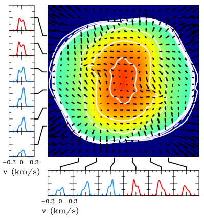
Figure 3.— The equatorial gas density, velocity, and CS(2-1) line profiles of the quadrupolar mode after the first half-period, (left), and the second full period, (right). These correspond to the times marked by black squares in Figure 2. Despite having oscillated for nearly $5\times 10^{5}\,{\rm yr}$, the quadrupolar structure is still clearly evident in the density & velocity fields as well as in the spectral line profiles. Spectral line profiles colored blue (red) indicate approaching (retreating) gas on the near side relative to the observer.

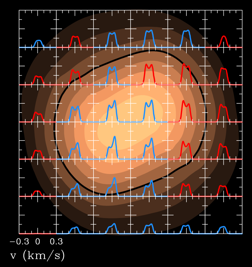
Figure 4.— A map of the CS(2-1) line profile overlaid upon the gas column density for the quadrupolar oscillation after nearly $5\times 10^{5}\,{\rm yr}$. This is viewed from $\lambda=30^{\circ}$, $\theta=30^{\circ}$, for which the pattern of spectral line profiles is similar to the Bok globule B68 (cf. Figure 7 of Keto et al. 2006). The gas density is shown as a filled contour map, with contours equally spaced in $10\%$ increments of the maximum value and the $50\%$ contour is marked by the thick black line. The CS(2-1) line profiles are associated with lines of sight centered in each subplot. Blue (red) lines correspond to approaching (retreating) gas on the nearside of the cloud relative to the observer. Note the prominent double reversal of the line-of-sight motions and the substantial distortion of the cloud shape, as seen in B68 (and in the same relative orientation).

Figure 5.— The dimensionless amplitude of the first dipole p-mode, the (1,1,1) mode. The dashed line is a quadratic fit to the logarithm of the amplitude, with an e-folding time of roughly $2\,{\rm M}{\rm yr}$ at $t=0$. The squares indicate the times for which the frames in Figure 6 were computed. The long-dashed line shows the $(0,2,2)$ mode, the only other significant oscillation.

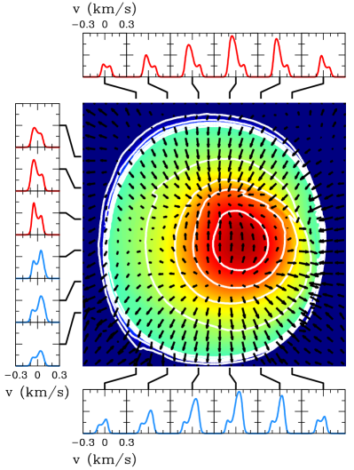
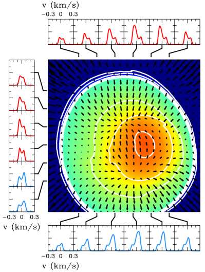
(a)	(b)

Figure 6.— The equatorial gas density, velocity, and CS(2-1) line profiles of the dipole mode after the first half-period, (a), and the second full period, (b). These correspond to the times marked by black squares in Figure 5. Despite having oscillated for more than $5\times 10^{5}\,{\rm yr}$, the dipolar structure is still clearly evident in the density & velocity fields as well as in the spectral line profiles. Spectral line profiles colored blue (red) indicate approaching (retreating) gas on the near side relative to the observer. Note that the spectra along the bottom would seem to imply expansion while those along the top would imply collapse. Furthermore, spectra from the side suggests rotation. Thus inferring the global state of the cloud from line profiles may be complicated by the presence of large-scale oscillations.

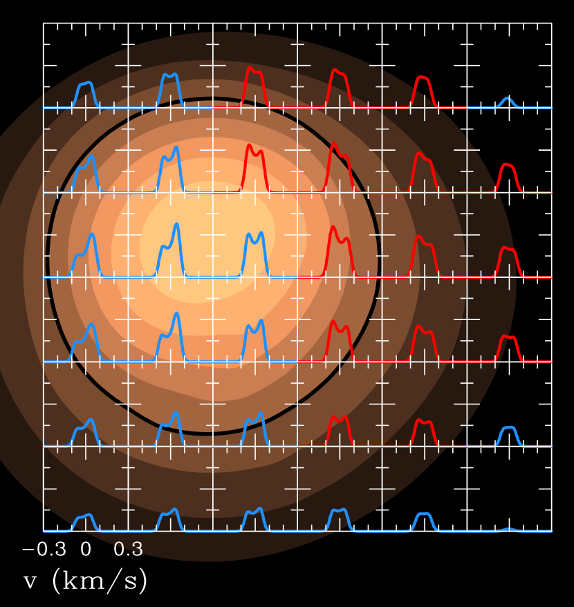
Figure 7.— A map of the CS(2-1) line profile overlaid upon the gas column density for the dipolar oscillation after more than $5\times 10^{5}\,{\rm yr}$. This is viewed from the same angle as shown in Figure 4, ($\lambda=30^{\circ}$, $\theta=30^{\circ}$). The gas density is shown as a filled contour map, with contours equally spaced in $10\%$ increments of the maximum value and the $50\%$ contour is marked by the thick black line. The CS(2-1) line profiles are associated with lines of sight centered in each subplot. Blue (red) lines correspond to approaching (retreating) gas on the nearside of the cloud relative to the observer. Note the prominent single reversal, similar to that associated with cloud rotation. For the dipole mode the distortion in the column density map is substantially less than that observed for the quadrupolar mode.

2.1. Hydrodynamic Evolution

Because the thermal gas heating and cooling time, via collisional coupling to dust at high densities (Burke & Hollenbach 1983) and molecular line radiation at low densities (Goldsmith 2001), is short in comparison to the typical oscillation period (on the order of $10^{5}\,{\rm yr}$), the oscillations of dark-starless cores are well modeled with an isothermal equation of state. In particular, we use a barotropic equation of state with an adiabatic index of unity, in which case the isothermal evolution is also adiabatic. Since the unbounded isothermal gas sphere is unstable, we truncate the solution at a given density contrast ($\rho(R)/\rho_{c}$), producing the standard Bonnor-Ebert sphere solution. This is done by inducing a phase change in the equation of state, i.e.,

$$P=\left\{\begin{aligned} \rho\frac{kT}{\mu m_{p}}&&&\text{if }\rho\geq\rho(R)\,,\\ \left[\frac{\rho}{\rho(R)}\right]^{\epsilon}\rho(R)\frac{kT}{\mu m_{p}}&&&\text{if }\rho(R)>\rho\geq\delta\rho(R)\frac{T}{T_{\rm ext}}\,,\\ \rho\frac{kT_{\rm ext}}{\mu m_{p}}&&&\text{otherwise}\,,\end{aligned}\right.$$ (1)

where the intermediate state, with $\delta=0.8$ and $\epsilon=\log(\delta)/\log(\delta T/T_{\rm ext})\ll 1$ chosen to make $P(\rho)$ continuous, is introduced to avoid numerical artifacts at the surface, and $T_{\rm ext}\gg T$. The resulting radial density and pressure profiles are shown in Figure 1. Note that there is a transition region, associated with the intermediate state in the equation of state, which distributes the sudden drop in density over many grid zones. Despite this, the pressure is continuous (necessarily) and nearly constant outside the surface of the Bonnor-Ebert sphere. We find that generally our results are insensitive to the particular equation of state of the exterior hot gas, given that it is sufficiently dilute. This is appropriate for globules like B68 which are known to be surrounded by hot, low density gas.

We employ a three-dimensional, self-gravitating hydrodynamics code to follow the long term mode evolution. Details regarding the numerical algorithm and specific validation for oscillating gas spheres (in that case a white dwarf) can be found in Broderick & Rathore (2006), and thus will only be briefly summarized here.

The code is a second order accurate (in space and time) Eulerian finite-difference code, and has been demonstrated to have a low diffusivity. Because the equation of state is barotropic, we use the gradient of the enthalpy instead of the pressure in the Euler equation since this provides better stability in the unperturbed configuration (Broderick & Rathore 2006). The Poisson equation is solved via spectral methods, with boundary conditions set by a multipole expansion of the matter on the computational domain.

In order to assess the suitability of the code for application to isothermal gas spheres we tested the stability to monopolar perturbations as a function of central-to-surface density contrast, finding instability for values above $13.5$. This is in approximate agreement with the prediction of instability for density constrasts above 14.3 (Foster & Chevalier 1993). The deviation from $14.3$ is likely due to the effective atmosphere produced by the exterior hot matter, and in particular the material in the transition region of the equation of state.

Henceforth, the specific physical parameters of the unperturbed model that we use, chosen to be roughly applicable to B68, are $\rho_{c}=1.185\times 10^{-18}\,{\rm g}{\rm c}{\rm m}^{-3}$, $\rho(R)/\rho_{c}=12.5$, and $T=10\,{\rm K}$. In all cases the simulations were performed at resolutions of $64^{3}$, $128^{3}$ and $256^{3}$. Comparison of the latter two indicated that the numerical solution had converged by these resolutions. The results presented in the following sections are from the simulations at $256^{3}$.

The initial perturbed states are computed in the linear approximation using the standard formalism of adiabatic (which in this case is also isothermal, Keto et al. 2006) stellar oscillations (Cox 1980). The initial conditions of the perturbed gas sphere are then given by the sum of the equilibrium state and the linear perturbation. We employ the same definition for the dimensionless mode amplitude as given in the Appendix of Keto et al. (2006).

Throughout the evolution, the amplitude of a given oscillation mode, denoted by its radial ($n$) and angular ($l$ & $m$) quantum numbers, may be estimated by the explicit integral:

$$A_{nlm}=\omega_{nlm}^{-1}\int{\rm d}^{3}\!x\,\rho\,\mbox{\boldmath$\rm v$}\cdot\mbox{\boldmath$\rm\xi$}_{nlm}^{\dagger}\,,$$ (2)

where $\rm v$ is the gas velocity, $\mbox{\boldmath$\rm\xi$}_{nlm}$ is the mode displacement eigenfunction, $\omega_{nlm}$ is the mode frequency and the dagger denotes hermitian conjugation.

2.2. Molecular Line Simulations

Assuming that the gas contains the usual interstellar molecules, we simulate molecular line observations of the hydrodynamic model by calculating the non-LTE (non-thermodynamic equilibrium) emission of the CS(2-1) transition using our three-dimensional ALI (accelerated $\Lambda$ iteration) code (Keto et al. 2004). The densities, velocities, and constant temperature are taken from the hydrodynamic simulation. The line broadening is assumed purely thermal.

The abundance of CS is based on a simplified model of CO chemistry from Keto & Caselli (2008). We briefly describe the model here. The abundance of CO in the gas is decreased by two effects, by photodissociation at the edge of the cloud and by freezing onto dust grains in the high density center. We calculate the reduction in the CO abundance due to these two affects and assume that the same reduction affects the CS molecule. We assume, as in Keto et al. (2006), an undepleted abundance of CS of $6\times 10^{-9}$. This is consistent with Tafalla et al. (2002), who cite a range in values derived from their observations of $3-9\times 10^{-9}$.

Tielens & Hollenbach (1985) suggest that at the edge of the cloud where photodissociation is important, the dominant cycle for the formation and destruction of CO is

$${\rm C}^{+}\rightarrow{\rm CH}_{2}\rightarrow{\rm CO}\rightarrow{\rm C}\rightarrow{\rm C}^{+}\,.$$ (3)

The time scale for the formation of CH₂ by radiative association is longer than for the formation of CO from CH₂ and O. Therefore we assume that the rate of formation of CO is given by that of CH₂. The CO cycle may then be described by three rate equations for the creation of C⁺, C, and CO plus the conservation condition that the total amount of carbon is contained in these three species. The rate equations for photodissociation depend on the mean visual extinction at each point, which we calculate using the machinery of the three-dimensional radiative transfer code.

The distribution of CO between the gas and grain phases is controlled by the rate of depletion from the gas phase by freezing onto dust grains and the rate of desorption off dust grains by cosmic rays. The steady state abundance of CO in the gas phase is then given by the ratio of the depletion time to the sum of the depletion and desorption times. Because the depletion time scales inversely with the collision rate while the desorption time scales inversely with the cosmic ray ionization rate, the depletion of CO is dependent only on the gas density because the cosmic ray ionization rate is the same throughout the cloud.

3. Quadrupole Perturbations

The primary mode discussed in Keto et al. (2006) was the first quadrupole p-mode, i.e., the $n=1$, $l=m=2$ oscillation mode. In order to reproduce the observed velocities it was necessary to consider a dimensionless amplitude of $0.25$, which produced near-vanishing densities in some portions of the cloud, and is thus clearly well into the non-linear regime.

The evolution of the dimensionless amplitude of the $(1,2,2)$ mode, as defined by equation (2), is shown as a function of time in Figure 2. The decay is well approximated by an exponential. However, the strongly non-linear nature of the decay is evident in the changing decay constant (resulting in a noticeable bowing of the fitted line in Figure 2), which yields an initial e-folding time of approximately $2\,{\rm M}{\rm yr}$, corresponding to roughly $8$ oscillation periods ($16$ pattern periods). Since the intrinsic dissipation in the code has previously been shown to be small (Broderick & Rathore 2006), the decay in the amplitude is dominated by non-linear mode interactions, resulting in the transfer of energy from large-scale, low-order modes to smaller-scale, higher-order modes . However, mass loss driven by large velocity perturbations and mode coupling in the artificial atmosphere (see Figure 1) also contribute to the decay. It is not clear if these processes are artifacts of our numerical simulation and the manner in which we initially prepare the cloud or if they may be found in nature as well. Thus our estimate of the lifetime should be considered a lower limit.

The only two oscillations of comparable wavelength (less than approximately $R/5$) that reach significant amplitudes are the $(0,2,2)$ and $(0,4,4)$ modes, whose couplings are likely enhanced by the Cartesian geometry of the underlying computational grid. In particular, there is no evidence for an inverse-cascade, implying that the gas cloud will not fragment. Indeed, this can be explicitly seen in the density and velocity structures in the equatorial plane (see Figure 3) in which the mode energy is primarily dissipated into small scale motions. Thus even vigorous oscillations (at least up to amplitudes of 25%) do not appear to be sufficient to split the cloud into a binary.

Despite the decay in amplitude, the quadrupole mode structure is still apparent in the density distribution of the cloud after a number of oscillation periods. This is also apparent in the substantially distorted H₂ column densities, shown in Figure 4 for a viewing angle that reproduces the generic features of B68 ($\theta$ and $\lambda$ corresponding to the lattitude and longitude, respectively, of the line of sight and oriented such that $\lambda=0^{\circ}$/$90^{\circ}$ corresponding to a view from the bottom/left of the page in Figure 3). Even after many oscillations the column density maps are generally qualitatively similar to observations of dark cores which often show clouds with an aspect ratio of approximately 2:1 (Ward-Thompson, Motte, & Andre 1999; Bacmann et al. 2000).

Similarly, the complex velocity patterns, as inferred from the shape of the CS(2-1) line profiles, are present after multiple oscillations. To the left and below the plots of the density and velocity structure in Figure 3, the CS(2-1) line profiles are shown for a number of lines of sight. Comparison of the early time and late time line profiles suggests that the small scale motions, the result of damping of the initial oscillation, do not significantly alter the line shapes or, as a direct consequence, the inferred line-of-sight velocity distribution throughout the cloud. Due to the intrinsically complex nature of the oscillation velocity field, the inferred velocity map can mimic expansion, contraction, rotation, or a combination of these. For example, the velocity patterns inferred by the line shapes shown in Figure 3 appear to correspond to rotation, while if these were rotated by $45^{\circ}$ (diagonal lines of sight) they would appear to correspond to expansion or contraction.

The structure of the inferred velocity map can become substantially more complex as we approach the pole (the polar angle $\theta$ approaches $0^{\circ}$). As seen in Figure 4, for $\theta\simeq 30^{\circ}$ and azimuthal angle $\lambda\simeq 30^{\circ}$ a quadrupolar oscillation can reproduce the general features of B68. This includes a double reversal of the line-of-sight velocity across the cloud (represented by the change from red to blue to red in the line profiles) and the significantly distorted gas column density. In fact, for the view shown, the relative orientation of the column density distortion and the velocity double reversal is similar to that observed in B68! This continues to be the case even after $5\times 10^{5}\,{\rm yr}$.

As anticipated in Keto et al. (2006), the qualitative features of the linear column density and velocity maps are still present in the non-linear computation. In particular, both the anisotropic nature of the column densities and the complex velocity structure persist for a number of oscillation periods. Nevertheless, the non-linear decay of the amplitude, and subsequent small scale motions, does become significant on timescales of a ${\rm M}{\rm yr}$ as evidenced by the decay of the mode amplitude in Figure 2. As a consequence, non-linear mode damping appears to be the dominant constraint upon whether such an oscillation can be clearly observed in velocity maps.

4. Dipole Perturbations

Although not explicitly considered in Keto et al. (2006), dipole oscillations are a possible alternative interpretation to rotation, and perhaps also capable of explaining the velocity structure of B68. For this reason we considered the first dipole p-mode, i.e., the $n=l=m=1$ oscillation mode, as well.

As a consequence of its longer wavelength, the amplitude of the dipole mode must be larger than that of the quadrupole oscillation mode to produce similar velocities. Hence, we chose a dimensionless amplitude of $0.5$. Similar to the quadrupole case, this is also likely to be strongly non-linear.

As in the quadrupole case, the dipole oscillation decays primarily into small scale motions. In both the quadrupole and dipole case the cloud sheds a few percent of its mass from the outer layers, contributing to the decay of the oscillation. In the dipole case this also produces a notable shift in the center of mass of the cloud as a result of the asymmetric mass loss through the boundary of the computational domain.

As with the quadrupolar oscillations the gas column densities are initially strongly distorted. However, in contrast to the quadrupole mode, after the first oscillation period (approximately $1.5\times 10^{5}\,{\rm yr}$) they have become roughly circular (see, e.g., Figure 7). This suggests that large amplitude dipole modes alone are insufficient to generate the observed anisotropy in the shapes of dark cores.

Figure 5 shows the evolution of the dimensionless amplitude for the first dipole p-mode. Again the evolving decay constant implies that this is a strongly non-linear process. However, in this case no oscillations with similar amplitudes develop within the duration of the simulation (the largest being the $(0,2,2)$ mode, which again is likely due to the Cartesian nature of the grid). The mode lifetime is on the order of $2\,{\rm M}{\rm yr}$, considerably longer than the mode oscillation period. As before, there is no indication of cloud fragmentation.

Nevertheless, the velocity maps inferred from the CS (2-1) line shapes, shown in Figures 6, retain their dipolar structure, even after many oscillations. Note that this implies that inferring the global dynamical state of the cloud from line profiles alone is significantly complicated by the possible existence of large-scale oscillations. As shown in Figures 6 & 7, for a variety of viewing angles, the motion appears to mimic rotation, expansion or contraction, all while in the same dynamical state. This is still true after the column density maps become nearly spherical.

5. Conclusions

Despite their strongly non-linear nature, large-amplitude oscillations of pressure-supported molecular clouds reproduce many of the qualitative features of observations of starless cores. These include the complex velocity structures and highly distorted column densities found in B68 and L1544, as well as mimicking rotation, expansion, and contraction depending upon the mode structure and viewing angle. This may complicate efforts to discern the global dynamical state of these objects from observations of molecular line shapes alone.

However, it may be possible to distinguish oscillations from collapse by comparing the spectral line profiles and velocities of volatile molecules such as N2H+ and NH3 against those of more refractory species such as CO, HCO+, or CS (Keto & Field 2005). In a simple breathing mode oscillation, the gas velocities are highest towards the outer regions of the cloud where the abundance of the carbon species is not depleted by freeze-out. In contrast, in the gravitational collapse of unstable BE spheres, the gas velocities are highest in the center of the cloud where the emission from the non-depleting nitrogen molecules is highest.

We note that we have restricted our attention to hydrodynamic oscillations of pressure-bounded, thermally-supported spheres. This description seems appropriate for globules such as B68 that are surrounded by hotter gas and have density profiles that closely match those of Bonnor-Ebert spheres. Whether the Bonnor-Ebert description is appropriate for embedded cores remains to be determined. For example, if magnetic stresses contribute significantly to cloud support, then additional classes of oscillations exist, associated with the magnetic field (see,e.g., Hennebelle 2003; Galli 2005).

The lifetimes of hydrodynamic oscillations of starless cores like B68 are sufficiently long (few $10^{6}$ yr) to be a significant fraction of the expected lifetime of a molecular cloud ($10^{7}$ yr). The oscillation lifetimes are dominantly limited by non-linear mode-mode coupling. Nevertheless, large amplitude oscillations persist for many periods (and thus many sound crossing times), and are therefore not expected to be particularly rare. There are no signs of cloud fragmentation, and thus amplitudes comparable to those discussed here are insufficient to produce binaries without the inclusion of additional physical processes.

References

- Alves, Lada, & Lada (2001) Alves, J., Lada, C., & Lada, E. 2001, Nature, 409, 159
- Bacmann et al. (2000) Bacmann, A., Andre, A.P., Puget, J.-L., Abergel, A., Bontemps, S. & Ward-Thompson, D. 2000, A&A, 361, 555
- Bergin et al. (2001) Bergin, E., Ciardi, D., Lada, C., Alves, J., Lada, E., 2001, ApJ, 557, 209
- Bok (1948) Bok, B., 1948, Centennial Symposia, Harvard Observatory Monographs No. 7, Harvard-College Observatory, Cambridge
- Broderick & Rathore (2006) Broderick, A. E. and Rathore, Y., 2006, MNRAS, 372, 923
- Burke & Hollenbach (1983) Burke, J. R. & Hollenbach, D. J., 1983, ApJ, 265, 223
- Caselli et al. (2002) Caselli, P., Walmsley, C., Zucconi, A., Tafalla, M., Dore, L. & Myers, P. 2002a, ApJ, 565, 331
- Cox (1980) Cox, J.P., 1980, Theory of Stellar Pulsations, Princeton University Press: Princeton
- Foster & Chevalier (1993) Foster, P. & Chevalier, R., 1993, ApJ, 416, 303
- Galli (2005) Galli, D., 2005, MNRAS, 359, 1083
- Goldsmith (2001) Goldsmith, P., 2001, ApJ, 557, 736
- Hennebelle (2003) Hennebelle, P., 2003, A&A, 411, 9
- Keto et al. (2004) Keto, E., Rybicki, G., Bergin, E., Plume, R., 2004, ApJ, 613, 355
- Keto & Field (2005) Keto, E. & Field, G., 2005, ApJ, 635, 1151
- Keto et al. (2006) Keto, E., Broderick, A., Lada, C.J. & Narayan, R., 2006, ApJ, 652, 1366
- Keto & Caselli (2008) Keto, E. & Caselli, P., 2008, in preparation
- Lada et al. (2003) Lada, C., Bergin, E., Alves, J., Huard, T., 2003, ApJ, 586, 286
- Tafalla et al. (2002) Tafalla, M., Myers, P., Caselli, P., Walmsley, C. & Comito, C., 2002, ApJ, 569, 815