Gauge Theory And Wild Ramification

Abstract.

The gauge theory approach to the geometric Langlands program is extended to the case of wild ramification. The new ingredients that are required, relative to the tamely ramified case, are differential operators with irregular singularities, Stokes phenomena, isomonodromic deformation, and, from a physical point of view, new surface operators associated with higher order singularities.

1. Introduction

The geometric Langlands program describes an analog in geometry of the Langlands program of number theory and is intimately connected with many topics in mathematical physics. It has been extensively studied via two-dimensional conformal field theory [4], [15], [16], and more recently via four-dimensional gauge theory with electric-magnetic duality [26]. That last paper contains more detailed references.

The gauge theory in question is a topologically twisted version of ${N}=4$ super Yang-Mills theory. As was first argued in [5], [19], electric-magnetic duality in this situation reduces in two dimensions to mirror symmetry of Hitchin fibrations [21], [22]. The particular case of mirror symmetry that is relevant here was first studied mathematically in [20].

The simplest form of the geometric Langlands program deals with a flat connection on a Riemann surface $C$. However, the analogy with number theory motivates the extension to incorporate “ramification,” that is to consider a flat connection on $C$ with singularities of a prescribed nature. The singularities may be simple poles, corresponding to “tame ramification,” or poles of higher order, in which case one speaks of “wild ramification.”

The gauge theory approach to tame ramification has been described in detail recently [18]. The main novelty, from a physics point of view, is the need to enrich ${N}=4$ super Yang-Mills theory with “surface operators,” which are characterized by prescribed singularities on codimension two surfaces in spacetime. The appropriate singularities appear in solutions of Hitchin’s equations with tame singularities; these solutions were first described in [34]. After supplementing the parameters that appear in the classical description of these singularities with certain quantum parameters (theta-like angles), it was possible in [18] to describe an action of electric-magnetic duality on a certain family of (half-BPS) supersymmetric surface operators. This led to a natural gauge theory description of the tame case of the geometric Langlands correspondence. For an elegant supergravity analysis of the relevant family of surface operators, see [17].

The purpose of the present paper is to extend the gauge theory approach to the case of wild ramification. This depends on overcoming two major obstacles and interpreting the results in quantum field theory. As it turns out, at the classical level the two obstacles have already been dealt with in the literature.

The first obstacle is that at first sight the higher order singularities relevant to wild ramification look incompatible with Hitchin’s equations. We can write Hitchin’s equations very schematically in the form $d\Phi+\Phi^{2}=0$, where $\Phi$ combines the connection and Higgs field (which we usually denote as $A$ and $\phi$, respectively). For now, it is not necessary to describe Hitchin’s equations more precisely. Tame ramification means that at a point on a Riemann surface that is labeled as $z=0$ in terms of some local parameter $z$, we have a singularity with $|\Phi|\sim 1/|z|$ (possibly up to logarithms). With this behavior of $\Phi$, both $d\Phi$ and $\Phi^{2}$ are of order $1/|z|^{2}$ for small $z$, so it is natural, as in [34], to look for solutions of Hitchin’s equations of this form.

But for wild ramification, we want $|\Phi|\sim 1/|z|^{n}$ with $n>1$, and then the equation $d\Phi+\Phi^{2}=0$ looks unnatural, as it seems that $\Phi^{2}$ will be more singular than $d\Phi$. As shown in [8], following earlier work [32], the resolution of this point is simply that the relevant singular behavior of Hitchin’s equations can be modeled by abelian solutions, in which $d\Phi$ and $\Phi^{2}$ both vanish. There is no problem in finding abelian solutions of Hitchin’s equations with poles of arbitrary order. It is perhaps surprising that abelian solutions (possibly twisted by an element of the Weyl group) are sufficient for modeling the local singularity, but this follows from classical facts about irregular singularities.

The second problem that must be overcome is particularly vexing at first sight, although again, the resolution involves facts that are known and are summarized or developed in [9]. In the unramified case, the geometric Langlands correspondence begins with a flat connection on a Riemann surface $C$. Such a flat connection has a topological interpretation, independent of the complex structure on $C$, since it determines a homomorphism to $G_{\mathbb{C}}$ of the fundamental group of $C$. Likewise, in the tamely ramified case, one deals with flat connections on a punctured Riemann surface $C^{\prime}=C\backslash\{p_{1},p_{2},\dots,p_{s}\}$ (that is, $C$ with the $s$ points $p_{1},p_{2},\dots,p_{s}$ omitted) whose singularities are simple poles at the punctures. Again, such a connection has a topological interpretation, in terms of a homomorphism to $G_{\mathbb{C}}$ of the fundamental group of $C^{\prime}$.

This is all in accord with the fact that the gauge theory approach to the geometric Langlands correspondence begins with a twisted topological field theory in four dimensions. The underlying topological invariance means that the ingredients that appear after reduction to two dimensions must have a topological interpretation.

In the wildly ramified case, however, the starting point is a flat connection whose singularities are poles of order greater than 1. Such flat connections depend on parameters that in general cannot be given a topological interpretation. For example, consider in the holomorphic setting a connection with a pole at $z=0$:

(1.1) $${\mathcal{A}}=dz\left(\frac{T_{n}}{z^{n}}+\frac{T_{n-1}}{z^{n-1}}+\dots+\frac{T_{1}}{z}+\dots\right).$$

Here $T_{1},T_{2},\dots,T_{n}$ are elements of $\mathfrak{g}_{\mathbb{C}}$, the Lie algebra of $G_{\mathbb{C}}$.

A flat connection on $C^{\prime}$ which is allowed to have singularities of this nature depends on more parameters, namely $T_{2},\dots,T_{n}$, than a flat connection with only simple poles. But whatever the order of the poles, the only obvious topological invariant of a flat connection is the monodromy, or in other words the representation of the fundamental group of $C^{\prime}$, that it determines. So the extra information associated with wild ramification does not appear to have any topological meaning.

Related to this, $T_{1}$, being the residue of the holomorphic differential $\mathcal{A}$, is independent of the choice of local parameter $z$. But the remaining elements $T_{i}$, $i\geq 2$, do depend on the choice of local parameter. So they scarcely can be meaningful parameters in a topological field theory.

The resolution of this conundrum involves the theory of Stokes phenomena in ordinary differential equations with irregular singularity. Some of the information contained in a flat connection with irregular singularity does have a topological meaning, in terms of a generalized monodromy that includes the Stokes matrices. The remaining information that characterizes an irregular singularity can be varied by a natural process of isomonodromic deformation [25], preserving the generalized monodromy. A natural quantum field theory argument shows that the relevant information in our problem is invariant under isomonodromy.

The generalized monodromy parametrizes a variety that, just like the more familiar moduli spaces of representations of the fundamental group, has a natural complex symplectic structure. Moreover, and crucially for our application, this structure is invariant under isomonodromy [9], a fact which turns out to have a natural interpretation in ${N}=4$ super Yang-Mills theory. Additionally, the relevant variety can be interpreted [8] as a moduli space of solutions of Hitchin’s equations with a suitable singularity. This leads to a Hitchin fibration and mirror symmetry, just as in the unramified or tamely ramified case. This instance of mirror symmetry is related to four-dimensional gauge theory, and leads to the geometric Langlands duality, just as in those cases. The duality commutes with isomonodromic deformation.

Section 2 of this paper is devoted mainly to an introduction to Stokes phenomena; none of this material is new. However, section 2.9 contains a further explanation of the strategy of this paper.

In section 3, we introduce surface operators associated with wild ramification. In section 4, we offer a supersymmetric perspective on isomonodromy. Sections 5 and 6 describe the application to geometric Langlands. In section 5, we consider the case that the coefficient $T_{n}$ of the leading singularity is regular semi-simple; in section 6, this assumption is relaxed. Finally, some examples of Stokes phenomena are described in an appendix.

I would like to thank O. Biquard, P. Boalch, E. Frenkel, and D. Gaitsgory for explanations of their work and P. Deligne, S. Gukov, N. Hitchin, and I. M. Singer for helpful discussions.

2. Review Of Stokes Phenomena

We consider ${N}=4$ super Yang-Mills theory with gauge group $G$ on a four-manifold $M$ that is a product of Riemann surfaces, $M=\Sigma\times C$; $C$ is the Riemann surface on which we will study the geometric Langlands program. The theory works for any compact $G$, but for brevity we frequently take $G$ to be simple and connected.

The fields that will be important in the discussion are a connection $A$ on a $G$-bundle $E\to C$, and a field $\phi$ that is a one-form on $C$ with values in ${\rm ad}(E)$. Physically, $\phi$ arises by the twisting procedure applied to some of the scalar fields of ${N}=4$ super Yang-Mills theory. Asking for a pair $(A,\phi)$ to preserve supersymmetry gives Hitchin’s equations:

$$F-\phi\wedge\phi =0$$

(2.1) $$D\phi=D\star\phi =0.$$

Here $\star$ is the Hodge star operator.

Hitchin’s equations imply among other things that the complex-valued connection ${\mathcal{A}}=A+i\phi$ is flat, or in other words that its curvature ${\mathcal{F}}=d{\mathcal{A}}+{\mathcal{A}}\wedge{\mathcal{A}}$ vanishes. The gauge-covariant exterior derivative $d_{\mathcal{A}}$ can be decomposed as $d_{\mathcal{A}}=\partial_{\mathcal{A}}+\overline{\partial}_{\mathcal{A}}$, where $\partial_{\mathcal{A}}$ and $\overline{\partial}_{\mathcal{A}}$ are of types $(1,0)$ and $(0,1)$, respectively. The operator $\overline{\partial}_{\mathcal{A}}$ determines a complex structure on the bundle $E$, at least away from possible singularities.

The present section will be devoted to describing some aspects of the behavior in the presence of singularities. We consider a solution of Hitchin’s equations with a singularity at a point $p$. We choose a local coordinate $z$ so that $p$ is the point $z=0$. The bundle $E$ can be extended over $p$ as a holomorphic bundle, though not as a flat bundle. (The holomorphic extension is not quite unique, something that played an important role in [18] and will be incorporated below.) Like any holomorphic bundle, $E$ is trivial locally. Once a trivialization is picked in a neighborhood of $p$, the operator $\overline{\partial}_{\mathcal{A}}$ reduces in that neighborhood to the standard operator $\overline{\partial}=d\overline{z}\,\partial/\partial\overline{z}$. Flatness of the connection ${\mathcal{A}}$ is now equivalent to the statement that ${\mathcal{A}}_{z}$, defined by $\partial_{\mathcal{A}}=dz\left(\partial_{z}+{\mathcal{A}}_{z}\right)$, is holomorphic away from $p$. ${\mathcal{A}}_{z}$ may be singular at $p$, since the bundle $E$ is only flat away from $p$. We are interested in the case that the singularity of ${\mathcal{A}}_{z}$ is a pole:

(2.2) $${\mathcal{A}}_{z}=\frac{T_{n}}{z^{n}}+\frac{T_{n-1}}{z^{n-1}}+\dots+\frac{T_{1}}{z}+\dots$$

for some positive integer $n$. The last ellipses refer to regular terms.

Away from the point $z=0$, a covariantly constant section $\Psi$ of the flat bundle $E$ must be annihilated by $\overline{\partial}_{A}=\overline{\partial}$, and thus is holomorphic in the usual sense. It also must obey $\partial_{A}\Psi=0$ or

(2.3) $$\left(\frac{\partial}{\partial z}+{\mathcal{A}}_{z}\right)\Psi=0.$$

The differential equation (2.3) for the holomorphic object $\Psi$ is said to have a regular singularity at $z=0$ if $n=1$, and an irregular singularity if $n>1$.

In the rest of this section, we will give a brief synopsis of a few facts about linear differential equations with such an irregular singularity. We first explain a few basic facts about Stokes phenomena; much more can be found in classical references such as [36], [2]. Then we briefly describe the notion of isomonodromic deformation [25] and its symplectic nature [9]. (Papers [25] and [9] also contain introductions to the Stokes phenomena. See also [30], [31] for string theory papers with some applications of Stokes phenomena.) The aim is only to explain the minimum that is needed for the rest of this paper.

As in many treatments of irregular singularities, we will make in much of this paper the simplifying assumption that $T_{n}$ is regular and semisimple. If $G_{\mathbb{C}}$ is $SL(N,{\mathbb{C}})$ or $GL(N,{\mathbb{C}})$, this means that $T_{n}$ can be diagonalized and has distinct eigenvalues. For any simple $G_{\mathbb{C}}$, it means that $T_{n}$ can be conjugated to a Cartan subalgebra, and that the subgroup of $G_{\mathbb{C}}$ that commutes with $T_{n}$ is precisely $\mathbb{T}_{\mathbb{C}}$. Assuming that $T_{n}$ is regular and semisimple will enable us to describe a little more simply the main points of the gauge theory approach to wild ramification. In section 6, we sketch what is involved in relaxing the assumption about $T_{n}$.

In our very schematic introduction to Stokes phenomena, to avoid an inessential extra layer of abstraction, we will assume that $G_{\mathbb{C}}$ is $GL(N,{\mathbb{C}})$ or $SL(N,{\mathbb{C}})$. The general case is similar with triangular matrices replaced by elements of Borel subgroups. See section 2 of [10] for a brief explanation.

2.1. Preliminaries

$C^{*}$ will denote a small disc in the complex $z$-plane with the point $z=0$ omitted. We consider a differential equation with an irregular singularity at $z=0$. The first question to consider is up to what type of equivalences such singularities should be classified.

From a topological point of view, if we allow arbitrary gauge transformations, the only invariant of a flat connection on $C^{*}$ is the holonomy or monodromy around the origin. From a holomorphic point of view, the analogous statement is that, if we allow holomorphic gauge transformations of the holomorphic differential equation (2.3) that may have essential singularities at $z=0$, then the monodromy is the only invariant.

In fact, if the monodromy is trivial, then integrating along a path gives a $G_{\mathbb{C}}$-valued function $g(z)=P\exp\left(-\int_{z_{0}}^{z}{\mathcal{A}}(z^{\prime})\right)$. Here, the point $z$, the base-point $z_{0}$, and the path of integration are taken to lie in $C^{*}$; $g(z)$ is independent of the path because the monodromy vanishes. A gauge transformation by $g^{-1}$ sets ${\mathcal{A}}=0$. A similar procedure shows that any two holomorphic connections with the same monodromy are gauge-equivalent if we allow gauge transformations of this type.

However, in the case of an irregular singularity, $g(z)$ has an essential singularity at $z=0$. In studying irregular singularities, we do not want to allow gauge transformations with an essential singularity, since as we have just seen this will not lead to an interesting theory. Instead, we allow only gauge transformations that are meromorphic at $z=0$.

Stokes phenomena arise because there is a crucial difference between gauge transformations that are meromorphic in a neighborhood of $z=0$ and gauge transformations that can only be defined in a formal Laurent series near $z=0$. We will give a simple example to show why this must be so.

Given our assumption that the coefficient $T_{n}$ of the leading singularity is regular and semisimple, it is possible order by order in powers of $z$ to make ${\mathcal{A}}$ diagonal. In explaining why, we take $G_{\mathbb{C}}=SL(2,{\mathbb{C}})$ to keep the notation simple. Since $T_{n}$ is regular and semisimple, we have

(2.4) $${\mathcal{A}}_{z}=\frac{1}{z^{n}}\begin{pmatrix}w&0\\ 0&-w\\ \end{pmatrix}+\dots$$

where $w\not=0$, and the ellipses refer to terms less singular than $z^{-n}$. Consider a gauge transformation generated by

(2.5) $$\epsilon=\begin{pmatrix}0&\sum_{r=1}^{\infty}f_{r}z^{r}\\ \sum_{r=1}^{\infty}g_{r}z^{r}&0\\ \end{pmatrix},$$

with formal power series $\sum_{r=1}^{\infty}f_{r}z^{r}$ and $\sum_{r=1}^{\infty}g_{r}z^{r}$. Under a gauge transformation, to first order ${\mathcal{A}}$ transforms by $\delta{\mathcal{A}}=-\partial_{\mathcal{A}}\epsilon=-\partial\epsilon/\partial z-[{\mathcal{A}}_{z},\epsilon].$ For $n>1$ (or for $n=1$ if $2w\notin\mathbb{Z}$) the coefficients $f_{r}$ and $g_{r}$ can be determined inductively to set the off-diagonal part of ${\mathcal{A}}$ to zero. The key point is that, since $w\not=0$, for any $a,b$ (representing off-diagonal terms in ${\mathcal{A}}$ that we wish to eliminate) one can find $f,g$ (two of the coefficients in eqn. (2.5)) such that

(2.6) $$\left[\begin{pmatrix}w&0\\ 0&-w\\ \end{pmatrix},\begin{pmatrix}0&f\\ g&0\\ \end{pmatrix}\right]=\begin{pmatrix}0&a\\ b&0\\ \end{pmatrix}.$$

Now, let us see why the formal power series that diagonalizes ${\mathcal{A}}$ cannot possibly converge, in general, in any neighborhood of $z=0$. To illustrate the point, we will consider a special case with ${\mathcal{A}}_{z}=T_{2}/z^{2}+T_{1}/z$ exactly. Moreover, we diagonalize $T_{2}$ as in (2.4), and write out $T_{1}$ as an explicit $2\times 2$ matrix:

(2.7) $${\mathcal{A}}_{z}=\frac{1}{z^{2}}\begin{pmatrix}w&0\\ 0&-w\\ \end{pmatrix}+\frac{1}{z}\begin{pmatrix}v&b\\ c&-v\\ \end{pmatrix}.$$

We write $T_{1,D}={\rm diag}(v,-v)$ for the diagonal part of $T_{1}$. The formal diagonalization procedure replaces ${\mathcal{A}}_{z}$ by

(2.8) $${\mathcal{A}}^{\prime}_{z}=\begin{pmatrix}\frac{w}{z^{2}}+\frac{v}{z}+\dots&0\\ 0&-\frac{w}{z^{2}}-\frac{v}{z}-\dots\\ \end{pmatrix},$$

where the point is that modulo regular terms, ${\mathcal{A}}^{\prime}_{z}$ coincides with the diagonal part of ${\mathcal{A}}_{z}$. The regular terms in ${\mathcal{A}}^{\prime}_{z}$ do not coincide with the analogous diagonal terms in ${\mathcal{A}}_{z}$.

Because ${\mathcal{A}}^{\prime}_{z}$ is diagonal, the monodromy of the modified connection ${\mathcal{A}}^{\prime}$ is trivial to compute and is $\exp(-2\pi iT_{1,D})$. However, this does not coincide with the monodromy of the original connection ${\mathcal{A}}$. In fact, the conjugacy class of the monodromy of ${\mathcal{A}}$ is easily determined. Because ${\mathcal{A}}$ is holomorphic throughout the whole punctured $z$-plane, its monodromy around $z=0$ can be evaluated on a large circle at infinity. To do so, we observe that ${\mathcal{A}}=T_{2}/z^{2}+T_{1}/z$ can be replaced by ${\mathcal{A}}^{\prime\prime}=T_{1}/z$, since $T_{2}/z^{2}$ vanishes too rapidly near infinity to contribute to the monodromy. The monodromy of ${\mathcal{A}}^{\prime\prime}$ is just $\exp(-2\pi iT_{1})$, and this gives the conjugacy class of the monodromy of ${\mathcal{A}}$.

Generically, $\exp(-2\pi iT_{1})$ and $\exp(-2\pi iT_{1,D})$ are not conjugate, so the holonomies of ${\mathcal{A}}$ and ${\mathcal{A}}^{\prime}$ are different. What has gone wrong with the reduction from ${\mathcal{A}}$ to ${\mathcal{A}}^{\prime}$ is that the formal power series used to diagonalize ${\mathcal{A}}$ has zero radius of convergence. (This can be verified explicitly in some examples treated in the appendix.)

To classify irregular singularities, we want to consider not formal power series, but only gauge transformations that are meromorphic in a punctured neighborhood of $z=0$. By such a gauge transformation, we cannot make ${\mathcal{A}}$ diagonal. But there is no problem with the diagonalization procedure up to any desired finite order. In particular, given that $T_{n}$ was assumed to be regular semisimple, we can assume ${\mathcal{A}}_{z}$ to take the form

(2.9) $${\mathcal{A}}_{z}=\frac{T_{n}}{z^{n}}+\frac{T_{n-1}}{z^{n-1}}+\dots+\frac{T_{1}}{z}+{\mathcal{B}},$$

where $T_{n},\dots,T_{1}$ are diagonal and ${\mathcal{B}}$ is regular at $z=0$. It is convenient to write

(2.10) $$\frac{T_{n}}{z^{n}}+\frac{T_{n-1}}{z^{n-1}}+\dots+\frac{T_{1}}{z}={\rm diag}(R_{1}(z),R_{2}(z),\dots,R_{N}(z)),$$

with explicitly

(2.11) $$R_{j}(z)=\frac{q_{jn}}{z^{n}}+\frac{q_{j,n-1}}{z^{n-1}}+\dots+\frac{q_{j1}}{z},~{}~{}j=1,\dots,N.$$

Further, we let

(2.12) $$Q_{j}(z)=\frac{q_{jn}}{(n-1)z^{n-1}}+\frac{q_{j,n-1}}{(n-2)z^{n-2}}+\dots+{q_{j1}}(-\ln z),$$

so that $dQ_{j}/dz=-R_{j}$. To define $Q_{j}$, it is necessary to pick a branch of $\ln z$, but the choice will not be important.

Even after making them diagonal, the matrices $T_{n},T_{n-1},\dots,T_{1}$ are not quite uniquely determined. A meromorphic gauge transformation by

(2.13) $$g={\rm diag}(z^{s_{1}},z^{s_{2}},\dots,z^{s_{N}})$$

with integer exponents would change the eigenvalues of $T_{1}$ by the integers $s_{1},s_{2},\dots,s_{N}$. Once we pick a particular $T_{1}$, we can limit ourselves to gauge transformations that are holomorphic and invertible at $z=0$. Making a choice of $T_{1}$ is equivalent to picking a particular holomorphic extension over the singular point at $z=0$ of the original flat bundle $E$ on the punctured disc $C^{*}$. After picking such an extension, we are still free to modify ${\mathcal{A}}$ by permuting the eigenvalues of $T_{n}$, that is, by a Weyl transformation, and by holomorphic gauge transformations that are diagonal up to order $z^{n}$. In particular, we can make a gauge transformation by a constant diagonal matrix, and this will be important later in counting parameters.

2.2. Stokes Rays

Now we want to study covariantly constant sections $\Psi$ of the flat bundle $E$, or equivalently holomorphic sections that obey the differential equation $(\partial_{z}+{\mathcal{A}}_{z})\Psi=0$. If $\mathcal{B}=0$ in (2.9), then a basis of such sections is given by

(2.14) $$\Psi_{j}=h_{j}\,\exp(Q_{j}(z)),~{}~{}j=1,\dots,N,$$

where the column vector $h_{j}$ has a 1 in the $j^{th}$ position, with other entries zero. In general, with $\mathcal{B}$ regular at $z=0$ but not necessarily zero, there is for each $j$ a unique formal power series $H_{j}(z)=h_{j}+{\mathcal{O}}(z)$ such that a basis of solutions (in a formal power series) is given by

(2.15) $$\Psi_{j}(z)=H_{j}(z)\exp(Q_{j}(z)).$$

The existence of the formal power series $H_{j}(z)$ is more or less equivalent to the statement that a gauge transformation diagonalizing ${\mathcal{A}}$ can be found as a formal power series. All entries of $H_{j}(z)$ are non-zero in general, but $H_{j}(0)=h_{j}$.

If the series $H_{j}$ have nonzero radii of convergence, the monodromy of the flat connection ${\mathcal{A}}$ can be computed from the covariantly constant sections (2.15) and equals $\exp(-2\pi iT_{1})$. For this reason, $T_{1}$ is known as the exponent of formal monodromy of the connection ${\mathcal{A}}$. As we have seen, in general the actual monodromy does not coincide with $\exp(-2\pi iT_{1})$, so the formal power series $H_{j}$ are not convergent.

Before proceeding, we need to discuss the asymptotic behavior near $z=0$ of the functions $\exp(Q_{j})$. This is determined by the real part of the leading terms $q_{j}/(n-1)z^{n-1}$ in the $Q_{j}$. Whether the real part of this expression is positive or negative depends on the direction that one approaches the point $z=0$ in the complex plane. We say that a “Stokes ray” of type $(ij)$ is a ray in the complex plane along which $(q_{i}-q_{j})/z^{n-1}$ takes values on the negative imaginary axis. The sign of $q_{ij}={\rm Re}\left((q_{i}-q_{j})/z^{n-1}\right)$ changes from positive to negative as $z$ crosses the Stokes ray in the counterclockwise direction. So “before” crossing the Stokes ray, one has $|\exp(Q_{i}(z))|>>|\exp(Q_{j}(z))|$ for $z\to 0$, while “after” crossing it (in the counterclockwise direction) this inequality is reversed. There are a total of $n-1$ Stokes rays of type $(ij)$, for each ordered pair $i,j$, as sketched in fig. 1.

Figure 1. For each pair $i,j$, there are $n-1$ Stokes rays of type $(ij)$ and an equal number of type $(ji)$. They alternate and are equally spaced, as shown here for $n=4$. To avoid clutter, only the Stokes rays associated with one pair $i,j$ are shown.

By an angular sector in the disc $C^{*}$, we mean a sector defined by $\theta_{a}\leq{\rm Arg}\,z\leq\theta_{b}$, for some $\theta_{a},$ $\theta_{b}$. A basic result about differential equations with irregular singularities is that in any sufficiently small angular sector $S$ in the complex $z$-plane, after possibly replacing $C^{*}$ by a smaller disc around the origin, there are holomorphic sections $\widehat{H}_{j,S}$, asymptotic to $H_{j}$ as $z\to 0$ in the sector $S$, such that

(2.16) $$\Psi_{j,S}=\widehat{H}_{j,S}\exp(Q_{j}(z))$$

give a basis of covariantly constant sections of the bundle $E$. (For some explicit examples of construction of the $\widehat{H}_{j,S}$ in simple cases, and verification of their asymptotic behavior, see the appendix.) For the case that $T_{n}$ is regular and semisimple, this is part of Theorem 12.3 of [36], which also asserts that the $\Psi_{j,S}$ exist with the claimed asymptotic behavior as long as

(2.17) $$\theta_{b}-\theta_{a}\leq{\pi\over n-1}.$$

The importance of the value in (2.17) will become clear. The generalization in which $T_{n}$ is not assumed to be regular and semisimple is Theorem 19.1 of [36]. (In the generalization, one needs to suitably modify the definition of $Q_{j}$ and $H_{j}$ to reflect the asymptotic behavior of solutions of the differential equation.)

Since $H_{j,S}=h_{j}+{\mathcal{O}}(z)$, the fact that $\widehat{H}_{j,S}$ is asymptotic to $H_{j,S}$ for small $z$ implies that

(2.18) $$\Psi_{j,S}\sim h_{j}\exp(Q_{j}(z)),~{}~{}z\to 0.$$

Now let us determine to what extent the $\Psi_{j,S}$ are uniquely determined by their asymptotic behavior (plus the differential equation that they obey). If $q_{jk}>0$, then $|\exp(Q_{j}(z))|>>|\exp(Q_{k}(z))|$ for small $z$. This being so, we can add to $\Psi_{j,S}$ a multiple of $\Psi_{k,S}$ without changing its asymptotic behavior for $z\to 0$ in the sector $S$. We cannot do the opposite; adding to $\Psi_{k,S}$ a multiple of $\Psi_{j,S}$ would change its asymptotic behavior for $z\to 0$. If the sector $S$ contains no Stokes rays, we can order the eigenvalues of $T_{n}$ so that throughout $S$, $q_{jk}>0$ if $j>k$. In that case, the indeterminacy is precisely that we can add to each $\Psi_{j,S}$ a linear combination of the $\Psi_{k,S}$ with $k<j$. Equivalently, the row vector

(2.19) $$\begin{pmatrix}\Psi_{1,S}&\Psi_{2,S}&\cdots&\Psi_{N,S}\\ \end{pmatrix}$$

can be multiplied on the right by an upper triangular matrix

(2.20) $$M=\begin{pmatrix}1&*&*&\dots&*\\ 0&1&*&\dots&*\\ 0&0&1&\dots&*\\ &&\ddots&&\\ 0&0&0&\dots&1\\ \end{pmatrix}$$

An $N\times N$ matrix $Y$ whose columns are a basis of solutions of the differential equation $(\partial_{z}+{\mathcal{A}}_{z})\Psi=0$ is called a fundamental matrix solution. For example, we can take $Y$ to have columns $\Psi_{1,S},\Psi_{2,S},\dots,\Psi_{N,S}$. Write $H$ for the matrix of formal power series whose columns are $H_{1},H_{2},\dots,H_{N}$, so in particular $H=1$ at $z=0$. And write $Q$ for the matrix $Q={\rm diag}(Q_{1},Q_{2},\dots,Q_{N})$. Then the asymptotic behavior for $z\to 0$ in the sector $S$ of the fundamental matrix solution $Y$ is

(2.21) $$Y\sim H\exp(Q).$$

The result of the last paragraph can be restated to say that a fundamental matrix solution with this asymptotic behavior is unique up to $Y\to YM$, where $M$ is a constant matrix, and, as in (2.20), $M-1$ is strictly upper triangular. (In the general theory, for an arbitrary simple Lie group, $M$ takes values in the unipotent radical of a suitable Borel subgroup, as explained in [10], section 2.)

Now suppose instead that the sector $S$ contains a Stokes ray of type $(ij)$ or $(ji)$. Then $\Psi_{i,S}$ and $\Psi_{j,S}$ exchange dominance in crossing the Stokes ray. So we cannot add a multiple of one to the other without spoiling the asymptotic behavior on one side or the other of the Stokes ray. Thus, if $S$ contains a Stokes ray, the indeterminacy of the solutions $\Psi_{i,S}$ is reduced.

For an important application of this, pick a sector $S$ whose boundary rays are not Stokes rays and whose angular width is precisely $\pi/(n-1)$, the maximum value in eqn. (2.17). This is the same as the spacing between adjacent Stokes rays of type $(ij)$ and $(ji)$. So for each unordered pair $i,j$, the sector $S$ contains precisely one Stokes ray of one of these two type, and we cannot change either $\Psi_{i,S}$ or $\Psi_{j,S}$ by a multiple of the other. Hence, in a sector $S$ of this special type, the solutions $\Psi_{i,S}$ of the differential equation are uniquely determined by their required asymptotic behavior.

It is important to clarify exactly what this uniqueness means. Once we pick a holomorphic extension of the bundle $E$ over the singular point, and further make a gauge transformation to put the connection in the form (2.9), the $\Psi_{i,S}$ are uniquely determined. The condition (2.18) that determines $\Psi_{i,S}$ is preserved by a gauge transformation that is 1 at $z=0$. But in general, a gauge transformation that preserves the form (2.9) need not be 1 at $z=0$; rather, at $z=0$, it can be an arbitrary (invertible) diagonal matrix – that is, an element of the complex maximal torus ${\mathbb{T}}_{\mathbb{C}}$ of $G_{\mathbb{C}}$. The choice of the $\Psi_{i,S}$ is not invariant under the action of ${\mathbb{T}}_{\mathbb{C}}$, and we will have to allow for this in classifying irregular singularities.

2.3. Enlarging The Sector

Let $\Psi_{i,S}$ and $\Psi_{j,S}$ be as above and suppose that the sector $S$ contains a Stokes ray of type $(ij)$. And let $\widetilde{\Psi}_{i,S}=\Psi_{i,S}+\lambda\Psi_{j,S}$ for some constant $\lambda$. Consider the asymptotic behavior of $\widetilde{\Psi}_{i,S}$ along a ray $\ell$ that approaches $z=0$ in the sector $S$.

Let us suppose that $q_{ij}>0$ if $\ell$ is “before” the Stokes ray (in a counterclockwise sense). Then in that region $\exp(Q_{j})$ is subdominant relative to $\exp(Q_{i})$, so $\widetilde{\Psi}_{i,S}$ has the same asymptotic behavior as $\Psi_{i,S}$:

(2.22) $$\widetilde{\Psi}_{i,S}\to H_{i}\,\exp(Q_{i}),~{}z\to 0.$$

But if $\ell$ is “after” the Stokes ray, the term $\lambda\Psi_{j,S}$ dominates $\widetilde{\Psi}_{i,S}$ for $z\to 0$, and the asymptotic behavior is

(2.23) $$\widetilde{\Psi}_{i,S}\to\lambda H_{j}\,\exp(Q_{j}),~{}z\to 0.$$

This demonstrates an important phenomenon: the asymptotic behavior of a solution of the differential equation for $z\to 0$ can change as one crosses a Stokes ray.

This statement has an equally important converse: the asymptotic behavior of such a solution can change only in crossing a Stokes ray. To see this, we consider a sector $S$ with sections $\Psi_{i,S}$ that obey the differential equation and the asymptotic condition (2.18), and we suppose that one of the boundary lines $\ell_{0}$ of sector $S$ is not a Stokes ray. We want to show that under this condition, the $\Psi_{i,S}$ can be analytically continued beyond $\ell_{0}$, with the asymptotic condition remaining valid. We order the eigenvalues of $T_{n}$ so that along $\ell_{0}$,

(2.24) $$q_{ij}>0~{}{\rm for}~{}i>j.$$

Let $\widetilde{S}$ be a sector containing $\ell_{0}$ in its interior and sufficiently small to contain no Stokes ray. The latter condition ensures that eqn. (2.24) holds throughout $\widetilde{S}$. Also, it means that $\widetilde{S}$ is sufficiently small that we can invoke Theorem 12.3 of [36] and find solutions $\Psi_{i,\widetilde{S}}$ of the differential equation in sector $\widetilde{S}$ obeying the asymptotic condition (2.18) in that sector. The intersection $S\cap\widetilde{S}$ is non-empty, and in this sector, the $\Psi_{i,S}$ are related to $\Psi_{i,\widetilde{S}}$ by a triangular matrix, as in eqn. (2.20):

(2.25) $$\begin{pmatrix}\Psi_{1,S}&\Psi_{2,S}&\cdots&\Psi_{N,S}\\ \end{pmatrix}=\begin{pmatrix}\Psi_{1,\widetilde{S}}&\Psi_{2,\widetilde{S}}&\cdots&\Psi_{N,\widetilde{S}}\\ \end{pmatrix}\begin{pmatrix}1&*&*&\dots&*\\ 0&1&*&\dots&*\\ 0&0&1&\dots&*\\ &&\ddots&&\\ 0&0&0&\dots&1\\ \end{pmatrix}$$

Since the $\Psi_{i,\widetilde{S}}$ are holomorphic in the sector $\widetilde{S}$, this gives an analytic continuation of the $\Psi_{i,S}$ throughout $\widetilde{S}$. Since the condition (2.24) holds throughout $\widetilde{S}$, the fact that the $\Psi_{i,\widetilde{S}}$ obey the asymptotic condition (2.18) throughout $\widetilde{S}$ plus the fact that the $\Psi_{i,S}$ are related to them by an upper triangular matrix means that $\Psi_{i,S}$ obey the asymptotic condition throughout $\widetilde{S}$.

This process can be continued until a Stokes ray is reached. Even in crossing a Stokes ray, the above argument for analytic continuation still works; but the asymptotic condition (2.18) fails, since if $\widetilde{S}$ contains a Stokes ray, we cannot assume (2.24) throughout $\widetilde{S}$.

2.4. Stokes Matrices

Pick a sector $S^{0}_{1}$ of angular width $\pi/(n-1)$ whose boundary rays are not Stokes rays. By rotating it through an angle that is an integer multiple of $\pi/(n-1)$, we get $2n-1$ additional sectors $S^{0}_{2},S^{0}_{3},\dots,S^{0}_{2n-2}$. Each of these has width $\pi/(n-1)$ and boundary rays that are not Stokes rays.

In each of the sectors $S_{\alpha}^{0}$, $\alpha=1,\dots,2n-2$, there are solutions of the differential equation $\Psi_{j,\alpha},~{}j=1,\dots,N$ that are uniquely determined by requiring that they obey the asymptotic condition (2.18) in the sector $S^{0}_{\alpha}$. Each of these can be continued to angular sectors $S_{\alpha}$ that are slightly larger than $S^{0}_{\alpha}$, still obeying the same asymptotic condition. The sectors $S_{\alpha}$ are wide enough to give a covering of the punctured disc.

We can label the eigenvectors of $Q$ and the $S_{\alpha}$ so that the inequalities (2.24) are obeyed on the intersection $S_{\alpha}\cap S_{\alpha+1}$ if $\alpha$ is odd. In that case, if $\alpha$ is even, the opposite inequalities are obeyed on $S_{\alpha}\cap S_{\alpha+1}$:

(2.26) $$q_{ij}>0~{}{\rm if}~{}i<j.$$

On each sector $S_{\alpha}$, we define a fundamental matrix solution $Y_{\alpha}$ whose columns are the $\Psi_{j,\alpha}$:

(2.27) $$Y_{\alpha}=\begin{pmatrix}\Psi_{1,\alpha}&\Psi_{2,\alpha}&\cdots&\Psi_{N,\alpha}\\ \end{pmatrix}.$$

On the intersection of the two sectors $S_{\alpha}$ and $S_{\alpha+1}$, the two fundamental matrix solutions $Y_{\alpha}$ and $Y_{\alpha+1}$, which both obey the same asymptotic condition, are related by

(2.28) $$Y_{\alpha+1}=Y_{\alpha}M_{\alpha}.$$

Here $M_{\alpha}$ is a triangular matrix with 1’s on the diagonal. It is upper triangular if $\alpha$ is odd (and the inequalities (2.24) are obeyed on $S_{\alpha}\cap S_{\alpha+1}$). It is lower triangular if $\alpha$ is even (and the opposite inequalities (2.26) are obeyed on the intersection).

The matrices $M_{\alpha}$ are known as Stokes matrices (or Stokes multipliers). They are uniquely determined up to conjugation by a common diagonal matrix – which arises from the freedom to make a diagonal gauge transformation of the connection ${\mathcal{A}}$, preserving the form (2.9).

To compute the monodromy around the singularity at $z=0$, we must take the product of Stokes matrices $M_{2n-2}M_{2n-1}\cdots M_{1}$. But this is not quite the whole story. The asymptotic condition (2.18) determines the $z\to 0$ asymptotic behavior of the solutions $\Psi_{j,\alpha}$ in terms of $\exp(Q_{j}(z))$, which itself has a monodromy, because of the logarithmic term in $Q_{j}$. These logarithmic terms alone would lead to a monodromy $\exp(-2\pi iT_{1})$ (which is the monodromy of the formal solutions (2.15) that were constructed as formal power series times $\exp(Q_{j})$). The actual monodromy $\widehat{M}$ is the product of the monodromy built into the condition (2.18) times the monodromy coming from the product of the Stokes matrices:

(2.29) $$\widehat{M}=\exp(-2\pi iT_{1})M_{2n-2}M_{2n-1}\cdots M_{1}.$$

We think of the Stokes matrices and the exponent $T_{1}$ of formal monodromy, or equivalently the Stokes matrices and the actual monodromy $\widehat{M}$, as the generalized monodromy data near the singularity at $z=0$. To classify the generalized monodromy up to gauge equivalence, this data must be taken modulo the action of the diagonal matrices, that is the action of the maximal torus ${\mathbb{T}}_{\mathbb{C}}$. Let us count the parameters in the generalized monodromy in the neighborhood of a single irregular singularity.

In our derivation, the complexified gauge group $G_{\mathbb{C}}$ is $SL(N,{\mathbb{C}})$ or $GL(N,{\mathbb{C}})$. The complex dimension of $G_{\mathbb{C}}$, which we denote at ${\rm dim}\,G_{\mathbb{C}}$, is $N^{2}-1$ or $N^{2}$, and the rank, which we call $r$, is equal to $N-1$ or $N$. A pair $M_{\alpha}$, $M_{\alpha+1}$ of successive Stokes matrices depends on ${\rm dim}\,G_{\mathbb{C}}-r$ complex parameters, and we have $n-1$ such pairs. To this we must add $r$ parameters for the exponent of formal monodromy. But we must also subtract $r$ parameters for dividing by the action of ${\mathbb{T}}_{\mathbb{C}}$. So altogether in a local description near an irregular singularity, the generalized monodromy is parametrized by

(2.30) $$c_{n}=(n-1)({\rm dim}(G_{\mathbb{C}})-r)$$

complex parameters.

Though our derivation has been for $SL(N,{\mathbb{C}})$ or $GL(N,{\mathbb{C}})$, the general case is similar, as explained in [10], section 2. Groups of upper or lower triangular matrices are replaced with suitable Borel subgroups. Most of the discussion has a close analog for general $G$, and in particular the number of parameters in the generalized monodromy is still given by (2.30).

2.5. Classification Of Irregular Singularities

The Stokes matrices plus the diagonal matrix-valued function $Q$ give a complete set of local invariants of an irregular singularity. (We need not mention separately the exponent of formal monodromy as it appears in $Q$.)

To prove this last statement, suppose we are given two different connections ${\mathcal{A}}$ and $\widetilde{\mathcal{A}}$, that have the same Stokes matrices and the same $Q$. Let $S^{0}_{1}$ be a sector of angular width $\pi/(n-1)$ whose boundary rays are not Stokes rays for either connection, and as above rotate it to get additional sectors $S^{0}_{2},\dots,S^{0}_{2n-2}$, and thicken these slightly to sectors $S_{1},\dots,S_{2n-2}$ whose intersections contain no Stokes lines. The connections ${\mathcal{A}}$ and $\widetilde{\mathcal{A}}$ lead to two differential equations, each of which can be analyzed as above. Let $Y_{\alpha}$ and $\widetilde{Y}_{\alpha}$ be the fundamental matrix solutions of the two equations in sector $S_{\alpha}$ with asymptotic behavior

(2.31) $$Y_{\alpha} \sim H\exp(Q)$$

$$\widetilde{Y}_{\alpha} \sim\widetilde{H}\exp(Q),$$

where $H$ and $\widetilde{H}$ are formal power series with $H(0)=\widetilde{H}(0)=1$. We have

(2.32) $$Y_{\alpha+1}=Y_{\alpha}M_{\alpha},~{}~{}\widetilde{Y}_{\alpha+1}=\widetilde{Y}_{\alpha}M_{\alpha},$$

with by hypothesis the same Stokes matrices for the two connections. This implies that $g=Y_{\alpha}\widetilde{Y}_{\alpha}{}^{-1}$ is independent of $\alpha$. (This remains valid after going all the way around the circle, since the two exponents of formal monodromy are also the same.) Moreover, the asymptotic condition (2.31) shows that $g(0)=1$. $g$ is a gauge transformation that maps one connection $\widetilde{\mathcal{A}}$ to the other one ${\mathcal{A}}$.

This statement also has a converse. For given $Q$, one can find an ${\mathcal{A}}$ that realizes any required set of Stokes matrices. This is shown in [2], following [33].

2.6. A More Global View

Now we are going to embed this local description in a global context. We consider a compact Riemann surface $C$ of genus $g_{C}$ with a flat $G_{\mathbb{C}}$ bundle $E$ with connection ${\mathcal{A}}$. From a holomorphic point of view, the $(0,1)$ part of the connection endows $E$ with a holomorphic structure, and then the $(1,0)$ part of the connection is a holomorphic one-form, locally $dz\,{\mathcal{A}}_{z}$, valued in ${\rm ad}(E)$. We are interested in the case that this one-form has a pole of order $n$ near a point $p$. We want to describe the appropriate generalized monodromy data and count the parameters that it depends on. (The generalization to several irregular singularities is straightforward.)

First let us review what happens in the absence of the singularity. We pick a basepoint $q\in C$. We let $A_{1},\dots,A_{g}$ and $B_{1},\dots,B_{g}$ be loops (“$A$-cycles” and “$B$-cycles”) starting and ending at $q$ and generating in the usual way the first homology group of $C$. Taking the monodromy of ${\mathcal{A}}$ around the $A$-cycles and $B$-cycles, we get elements of $G_{\mathbb{C}}$ that we denote as $U_{1},\dots,U_{g}$ and $V_{1},\dots,V_{g}$. They obey one relation

(2.33) $$1=U_{1}V_{1}U_{1}^{-1}V_{1}^{-1}\cdots U_{g}V_{g}U_{g}^{-1}V_{g}^{-1}.$$

In addition, they are only defined up to conjugation by a common element of $G_{\mathbb{C}}$ (coming from the action of gauge transformations at the basepoint $q$). The number of complex parameters is therefore

(2.34) $$d_{\mathcal{Y}}=(2g-2)\,{\rm dim}(G).$$

This is the complex dimension of the moduli space ${\mathcal{Y}}$ of flat $G_{\mathbb{C}}$-bundles on $C$.

Figure 2. A Riemann surface $C$, here taken to be of genus $g_{C}=1$, with an irregular singularity at a point $p$. A basepoint is taken at $q$. Show are the Stokes rays near $p$ and the important paths in defining the generalized monodromy data.

Now we incorporate an irregular singularity at a point $p\in C$. Restricting to a small punctured disc $C^{*}$ containing $p$, we analyze the local behavior by covering $C^{*}$ with sectors $S_{1},\dots,S_{2n-2}$, as in section 2.4. Let $p_{1}$ be a point in the sector $S_{1}$. To describe a flat connection on $C$ up to gauge equivalence of the desired sort, we repeat the analysis with a few corrections to account for the singularity. We must include one more group element $W$ to account for parallel transport from $q$ to $p_{1}$ along some chosen path (fig. 2), and then according to (2.30) we have $c_{n}=(n-1)({\rm dim}(G)-r)$ parameters to account for the local behavior near $p$. These parameters comprise the monodromy $\widehat{M}$ on a small loop circling the singularity in the disc $C^{*}$, as well as the Stokes matrices $M_{\alpha}$ that involve the asymptotic behavior near $p$. So the total number of extra complex parameters required to describe the situation in the presence of an irregular singularity is

(2.35) $$\widehat{c}_{n}={\rm dim}(G)+c_{n}=n\,{\rm dim}(G)-(n-1)r.$$

The monodromy data $U_{i},V_{j},$ and $W$, together with the local data at the singularity, obey one relation, as was the case in the absence of the singularity. But now, instead of (2.33), this relation is more complicated:

(2.36) $$1= U_{1}V_{1}U_{1}^{-1}V_{1}^{-1}\cdots U_{g}V_{g}U_{g}^{-1}V_{g}^{-1}W\widehat{M}W^{-1}$$

$$= U_{1}V_{1}U_{1}^{-1}V_{1}^{-1}\cdots U_{g}V_{g}U_{g}^{-1}V_{g}^{-1}W\exp(-2\pi T_{1})M_{2n-2}M_{2n-1}\cdots M_{1}W^{-1}.$$

We have written this relation both in terms of the monodromy $\widehat{M}$ around the singular point, and more explicitly in terms of the formal monodromy and the Stokes matrices. And now, the group of equivalences that acts on this data is $G_{\mathbb{C}}\times{\mathbb{T}}_{\mathbb{C}}$, where the first factor acts by gauge transformations at $q$ and the second by gauge transformations at $p_{1}$. An element $g\in G_{\mathbb{C}}$ acts by $U_{i}\to gU_{i}g^{-1}$, $V_{i}\to gV_{i}g^{-1}$, and $W\to gW$. And an element $S\in{\mathbb{T}}_{C}$ acts by $W\to WS^{-1}$, $M_{\alpha}\to SM_{\alpha}S^{-1}$.

2.7. Topological Interpretation

As above, we write ${\mathcal{Y}}$ for the moduli space of $G_{\mathbb{C}}$-valued flat connections on $C$, up to gauge transformation. And we write ${\mathcal{Y}}^{*}$ for the space that parametrizes the generalized monodromy data in the presence of an irregular singularity at $p$ (or more generally in the presence of several irregular singularities).

${\mathcal{Y}}$ can be defined purely topologically, since it can be interpreted as a moduli space of representations of the fundamental group of $C$. The topological nature of ${\mathcal{Y}}$ is explicit in the equation (2.33), which does not depend on the complex structure of $C$. A flat connection up to gauge transformation is equivalent to a set of elements $U_{i},V_{j}\in G_{\mathbb{C}}$ obeying (2.33), up to conjugation. So ${\mathcal{Y}}$ can be defined purely in topological terms.

The same is true of ${\mathcal{Y}}^{*}$, though this may be surprising at first. To describe, up to isomorphism, the generalized monodromy data of a flat connection on $C\backslash p$ with an irregular singularity at $p$, we must specify a larger set of group elements, namely $U_{i},V_{j}\in G_{\mathbb{C}}$, $\exp(-2\pi iT_{1})\in{\mathbb{T}}_{\mathbb{C}}$, and the Stokes matrices $M_{\alpha}$; the latter take values in groups of unipotent upper or lower triangular matrices (or, for general $G_{\mathbb{C}}$, in the unipotent radicals of appropriate Borel subgroups). The number of these elements, the subgroups in which they take values, and the equation (2.36) that they obey are all completely independent of the complex structure on $C$. So ${\mathcal{Y}}^{*}$, like ${\mathcal{Y}}$, can be defined in purely topological terms. Moreover, except for the exponent of formal monodromy, ${\mathcal{Y}}^{*}$ is independent of the function $Q(z)$ that enters the description of the singularity.

What may make this surprising is that the whole discussion of Stokes matrices and generalized monodromy seems to depend on viewing $C$ as a complex manifold and considering the function $\exp(Q)$. However, if we change slightly the complex structure of $C$, the position of the point $p$, or the leading singular term $T_{n}/z^{n}$ of the connection (preserving the condition that $T_{n}$ is regular and semisimple), the Stokes rays will move, but they will not change in number. The Stokes matrices will still take values in the same group of upper or lower triangular matrices, and they will still appear in the same equation (2.36).

By comparing the additional variables that enter the description of ${\mathcal{Y}}^{*}$, relative to those that entered in describing ${\mathcal{Y}}$, we see that the difference in complex dimension between ${\mathcal{Y}}^{*}$ and ${\mathcal{Y}}$ is

(2.37) $$\widehat{c}_{n}={\rm dim}(G_{\mathbb{C}})+c_{n}=n\,{\rm dim}(G_{\mathbb{C}})-(n-1)r.$$

Though we have described the case of one irregular singularity, the generalization to the case of several such singularities is straightforward. Each singularity associated with a pole of order $n$ increases the dimension by $\widehat{c}_{n}$.

Let us compare this to the total number of parameters needed to describe an irregular singularity. If we permit the $(1,0)$ part of a connection ${\mathcal{A}}$ to have a pole of order $n$ at a point $p$, then the singular behavior takes the familiar form $T_{n}/z^{n}+T_{n-1}/z^{n-1}+\dots+T_{1}/z$, and is described by $n$ elements of the Lie algebra ${\mathfrak{g}}_{\mathbb{C}}$. In all it takes $n\,{\rm dim}\,G_{\mathbb{C}}$ parameters to specify $T_{1},\dots,T_{n}$.

Of a total of $n\,{\rm dim}\,G_{\mathbb{C}}$ parameters, the generalized monodromy data give a topological interpretation to $\widehat{c}_{n}=n\,{\rm dim}\,G_{C}-(n-1)r$ parameters. We seem to be left, for each irregular singularity, with $(n-1)r$ parameters that do not have a topological interpretation. What are these?

In our previous analysis, we have in fact encountered certain parameters associated with each irregular singularity that at least appear not to have a topological interpretation. As a preliminary step in the analysis, we picked a local parameter $z$ near the singularity, and put the connection in the form

(2.38) $${\mathcal{A}}_{z}=\frac{T_{n}}{z^{n}}+\frac{T_{n-1}}{z^{n-1}}+\dots+\frac{T_{1}}{z}+{\mathcal{B}},$$

with $T_{n},\dots,T_{1}\in{\mathfrak{t}}_{\mathbb{C}}$, the Lie algebra of ${\mathbb{T}}_{\mathbb{C}}$, and $\mathcal{B}$ regular. Here $T_{1}$ is independent of the choice of local coordinate, since it is the residue of the differential form $dz\,{\mathcal{A}}_{z}$. But $T_{2},\dots,T_{n}$ do depend on the choice of coordinate, so it would be hard to give them any topological interpretation. They depend on a total of

(2.39) $$\delta_{n}=(n-1)r$$

parameters, since ${\mathfrak{t}}_{\mathbb{C}}$ has dimension $r$. These are the parameters that characterize the irregular singularity and are not captured by the generalized monodromy. How to vary these parameters while keeping fixed the generalized monodromy is shown in the theory of isomonodromic deformation for irregular singularities, developed by Miwa, Jimbo, and Ueno [25].

2.7.1. Action Of Braid Group   

The assertion that ${\mathcal{Y}}$ or ${\mathcal{Y}}^{*}$ can be defined purely topologically must be clarified in one respect. Let us first give an analogy. If we vary the complex structure of $C$ slightly, ${\mathcal{Y}}$ in a natural sense does not vary. However, if we consider arbitrary families of complex structures on $C$, then ${\mathcal{Y}}$ will in general acquire a monodromy, involving an action of the mapping class group of $C$. For $C$ of genus zero and a flat connection with regular singularities, this type of deformation is described by Schlesinger’s equation; for example, see [29], [23]. Now let us consider varying the polar coefficients $T_{n},\dots,T_{2}$ of an irregular singularity. Let ${\mathfrak{t}}_{{\mathbb{C}}}^{\rm reg}$ be the space of regular elements of $\mathfrak{t}_{\mathbb{C}}$. The space ${\mathcal{Y}}^{*}$ can be defined for any $T_{n}\in{\mathfrak{t}}_{{\mathbb{C}}}^{\rm reg}$. As $T_{n}$ is varied, the spaces ${\mathcal{Y}}^{*}$ are locally constant – they vary as fibers of a flat bundle over ${\mathfrak{t}}_{{\mathbb{C}}}^{\rm reg}$. But globally there is a monodromy, via which the fundamental group of ${\mathfrak{t}}_{{\mathbb{C}}}^{\rm reg}$ acts on ${\mathcal{Y}}^{*}$. The monodromy arises because the choice of a sector $S_{1}$ that is not bounded by Stokes rays cannot be made globally. (But ${\mathfrak{t}}_{\mathbb{C}}^{\rm reg}$ can be covered by small open sets, in each of which one can make such a choice, so ${\mathcal{Y}}^{*}$ is naturally invariant under a small change of $T_{n}$.) The fundamental group of ${\mathfrak{t}}_{{\mathbb{C}}}^{\rm reg}$ is called the braid group of $G$; we will denote it as $B(G)$. Its monodromy action on ${\mathcal{Y}}^{*}$ was exploited in [10].

2.8. Isomonodromic Deformation And Symplectic Structure

In the theory of isomonodromic deformation [25], one constructs meromorphic differential equations by which one can vary the parameters contained in $T_{2},T_{3},\dots,T_{n}$ without changing the generalized monodromy. This description of isomonodromy has many applications in two-dimensional integrable systems. It may well be eventually relevant to geometric Langlands, but in this paper we will use instead (section 4) a gauge theory approach to isomonodromy, more similar to that in [9].

The possibility of isomonodromic deformation makes it clear that the complex structure of the variety ${\mathcal{Y}}^{*}$ that parametrizes the generalized monodromy data must be independent of $T_{2},\dots,T_{n}$. This particular point is clear more directly from the explicit description of ${\mathcal{Y}}^{*}$ via the equation (2.36), which does not depend on the choice of $T_{2},\dots,T_{n}$.

To go farther, we need to recall that the moduli space ${\mathcal{Y}}$ of homomorphisms of the fundamental group of $C$ to a simple complex Lie group $G_{\mathbb{C}}$ has (up to a multiplicative constant) a natural symplectic structure, which can be defined in gauge theory by the formula [1]

(2.40) $$\Omega=-{i\over 4\pi}\int_{C}\,{\rm Tr}\,\delta{\mathcal{A}}\wedge\delta{\mathcal{A}}.$$

(Here $-{\rm Tr}$ is an invariant quadratic form on the Lie algebra $\mathfrak{g}_{\mathbb{C}}$; we normalize it so that short coroots have length squared 2.) This is a symplectic structure in the holomorphic sense; $\Omega$ is a closed, holomorphic, and nondegenerate $(2,0)$-form with respect to the complex structure of ${\mathcal{Y}}$.

It was shown in [9], section 5, that in the presence of an irregular singularity, the same formula can be used to define a complex symplectic structure. But now we define the complex symplectic structure not on ${\mathcal{Y}}^{*}$, but rather on what we might call ${\mathcal{Y}}^{*}(T_{1})$, the subvariety of ${\mathcal{Y}}^{*}$ in which $T_{1}$, the exponent of formal monodromy, is kept fixed. The idea here is that in defining ${\mathcal{Y}}^{*}(T_{1})$, we keep fixed all the coefficients $T_{1},T_{2},\dots,T_{n}$ of singular terms in ${\mathcal{A}}$. $T_{2},\dots,T_{n}$ are kept fixed in defining ${\mathcal{Y}}^{*}$, and additionally $T_{1}$ is kept fixed in defining ${\mathcal{Y}}^{*}(T_{1})$. So, although ${\mathcal{A}}$ has a singularity, its variation $\delta{\mathcal{A}}$ does not, as a result of which the formula (2.40) makes sense and has its usual properties.

It is fairly obvious that the holomorphic symplectic form $\Omega$ on ${\mathcal{Y}}$ or ${\mathcal{Y}}^{*}(T_{1})$ does not depend on a choice of complex structure of $C$; indeed, no such complex structure is used in the definition (2.40). Also true, but much less obvious, is that the symplectic structure of ${\mathcal{Y}}^{*}(T_{1})$ does not depend on $T_{2},\dots,T_{n}$. This is the main result of [9] (see Theorems 7.1 and 7.3), where it is proved using gauge theory. For alternative approaches, see [37], [28], [11]. In applying ${N}=4$ super Yang-Mills theory to wild ramification, a natural quantum field theory explanation of the fact that the symplectic structure of ${\mathcal{Y}}^{*}(T_{1})$ is independent of $T_{2},\dots,T_{n}$ will emerge (section 4). When made explicit, this will lead to an argument similar to that in [9].

The complex structure and symplectic structure of ${\mathcal{Y}}^{*}(T_{1})$ do depend on $T_{1}$. The fact that one must hold $T_{1}$ fixed to define a symplectic manifold and that the resulting symplectic structure depends on $T_{1}$ has nothing to do with irregular singularities; these statements also hold for $n=1$, which is the case of a regular singularity. The fact that the complex and symplectic structures should naturally depend on $T_{1}$ will be clear in the quantum field theory approach.

For future use, let us note that since $T_{1}$ is kept fixed in defining ${\mathcal{Y}}^{*}(T_{1})$, the dimension of ${\mathcal{Y}}^{*}(T_{1})$ is less than that of ${\mathcal{Y}}^{*}$ by $r$, the rank of $G$. So from (2.37), we get that

(2.41) $${\rm dim}\,{\mathcal{Y}}^{*}(T_{1})={\rm dim}\,{\mathcal{Y}}+\widehat{c}_{n}-r=(2g-2){\rm dim}(G_{\mathbb{C}})+n({\rm dim}G_{\mathbb{C}}-r).$$

For example, for $G_{\mathbb{C}}=SL(2,{\mathbb{C}})$, we get

(2.42) $${\rm dim}\,{\mathcal{Y}}^{*}(T_{1})=6g-6+2n.$$

2.9. Strategy Of This Paper

Now we can explain the strategy of the present paper. In the process, it will hopefully become clearer why we have begun the paper with a review of the theory of Stokes phenomena.

Let us first recall what was done in [26] in the unramified case, or in [18] with tame ramification. If ${\mathcal{Y}}(G,C)$ denotes the moduli space of flat $G_{\mathbb{C}}$ bundles on $C$, with structure group $G_{\mathbb{C}}$, then to ${\mathcal{Y}}(G,C)$ we can associate a pair of topological field theories, namely the $B$-model defined using the natural complex structure of ${\mathcal{Y}}(G,C)$ and the $A$-model defined using the real symplectic structure ${\rm Re}\,\Omega$. These theories do not depend on the complex structure of $C$, since as a complex symplectic manifold, ${\mathcal{Y}}(G,C)$ has no such dependence. (These are actually two points in a larger family of topological field theories described in [26], and parametrized by ${\mathbb{CP}}^{1}$, but we will not emphasize the generalization in the present paper.)

Similarly, if we replace $G$ with the dual group ${}^{L}\negthinspace G$, we can define a $B$-model and an $A$-model with target ${\mathcal{Y}}({}^{L}\negthinspace G,C)$. One might wonder if there is some kind of duality between the topological field theories associated with $G$ and with ${}^{L}\negthinspace G$. But even once it is asked, this question is hard to answer without some additional structure.

However, if one interprets ${\mathcal{Y}}(G,C)$ and ${\mathcal{Y}}({}^{L}\negthinspace G,C)$ as moduli spaces of solutions of Hitchin’s equations, then one has a hyper-Kahler structure, and, using a different complex structure on these spaces (not the natural one that we have used up to this point) one can define the Hitchin fibration [21], [22]. As was first described mathematically in [20], the Hitchin fibration in this situation can be interpreted as a special Lagrangian fibration [35] that establishes a mirror symmetry between ${\mathcal{Y}}(G,C)$ and ${\mathcal{Y}}({}^{L}\negthinspace G,C)$.

This framework can be derived from four-dimensional ${N}=4$ super Yang-Mills theory with electric-magnetic duality, as first considered in [5], [19]. The idea of [26] was that by incorporating additional ingredients of the physics, such as the Wilson and ’t Hooft operators and various special branes, one can get a natural understanding of geometric Langlands duality. This duality maps a flat connection on $C$, with gauge group ${}^{L}\negthinspace G$, to a ${\mathcal{D}}$-module on the moduli space of $G$-bundles.

This approach was extended to the case of tame ramification in [18]. In this case, one must consider flat bundles with ramification (monodromy around marked points). The appropriate moduli spaces can again be interpreted [34] as moduli spaces of solutions of Hitchin’s equation. This leads to a Hitchin fibration and a mirror symmetry, and ultimately to an understanding of geometric Langlands duality by the same logic as in [26]. The details are a little more elaborate, however, because the dependence on the ramification parameters leads to the existence of noncommutative monodromy symmetries that commute with the duality.

In the present paper, we extend this to the case of wild ramification. Here, the basic symmetry is a mirror symmetry between the extended monodromy manifolds ${\mathcal{Y}}^{*}(T_{1})$ with gauge groups $G$ and ${}^{L}\negthinspace G$. The mirror symmetry follows as usual from the fact [8] that ${\mathcal{Y}}^{*}(T_{1})$ can be interpreted as a moduli space of solutions of Hitchin’s equations. The rest of the gauge theory machinery can then be applied, as in [26], to argue a geometric Langlands correspondence.

However, the fact that as a complex symplectic manifold, ${\mathcal{Y}}^{*}(T_{1})$ is independent of the parameters $T_{2},\dots,T_{n}$ that appear in a flat connection with irregular singularity shows that we must be careful in stating the geometric Langlands correspondence, if we want it to be a natural one-to-one correspondence between two kinds of object. Both the left and right hand sides of the correspondence are invariant under isomonodromic deformation, and the duality between them also commutes with isomonodromic deformation. Two flat ${}^{L}\negthinspace G_{\mathbb{C}}$ connections with irregular singularity that are equivalent under isomonodromic deformation have equivalent duals. So if we want the geometric Langlands correspondence to be a natural correspondence between two types of object, one approach might be to consider the starting point to be a flat ${}^{L}\negthinspace G_{\mathbb{C}}$ connection with irregular singularity, modulo isomonodromic deformation.

But this would force us to identify two flat connections with irregular singularity that have the same values of $T_{2},\dots,T_{n}$ and differ by the action of the braid group $B(G)$. This will probably not work nicely, since ${\mathcal{Y}}^{*}(T_{1})$ is unlikely to have a nice quotient by the action of $B(G)$. Hence, it is probably better not to try to divide by isomonodromic deformation but simply to assert that the duality commutes with such deformation. From an algebraic point of view, there is another reason to formulate things this way. The isomonodromy equations [25] are algebraic, but their solutions are not algebraic (in the usual algebraic structure relevant to geometric Langlands). So in the algebraic setting, isomonodromy gives an infinitesimal way of varying $T_{2},\dots,T_{n}$, commuting with geometric Langlands duality, but cannot be exponentiated to an actual map between objects with different values of $T_{2},\dots,T_{n}$.

3. Surface Operators With Wild Ramification

3.1. Local Model Of Abelian Singularity

As explained in section 2.9, to find a mirror symmetry for connections with irregular singularity, we need a relation between such connections and solutions of Hitchin’s equations:

$$F-\phi\wedge\phi =0$$

(3.1) $$D\phi=D\star\phi =0.$$

Consider an irregular singularity at a point $p$ defined as $z=0$ in terms of some local parameter $z$. Near $p$, the fields $A,\phi$ are more singular than $1/|z|$. Hitchin’s equations are schematically $d\Phi+\Phi^{2}=0$, where $\Phi=(A,\phi)$, and are not compatible with having $\Phi$ more singular than $1/|z|$ unless the singular parts of $d\Phi$ and $\Phi^{2}$ both vanish. This means that the singular part of the solution must be abelian. And indeed, this assumption leads to a good theory [32], [8] of solutions of Hitchin’s equations with irregular singularity.

We write $z=re^{i\theta}$, and we let $\mathfrak{t}$ denote the Lie algebra of a maximal torus $\mathbb{T}$ of the compact Lie group $G$, and $\mathfrak{t}_{\mathbb{C}}$ its complexification. We pick elements $\alpha\in\mathfrak{t}$ and $u_{1},\dots,u_{n}\in\mathfrak{t}_{\mathbb{C}}$, and consider the following explicit solution of Hitchin’s equations on a trivial $G$-bundle $E$ over the punctured complex $z$-plane:

(3.2) $$A =\alpha\,d\theta$$

$$\phi =\frac{dz}{2}\left(\frac{u_{n}}{z^{n}}+\frac{u_{n-1}}{z^{n-1}}+\dots+\frac{u_{1}}{z}\right)+\frac{d\overline{z}}{2}\left(\frac{\overline{u}_{n}}{\overline{z}^{n}}+\frac{\overline{u}_{n-1}}{\overline{z}^{n-1}}+\dots+\frac{\overline{u}_{1}}{\overline{z}}\right).$$

$\overline{u}_{k}$ is the complex conjugate of $u_{k}$, so $\phi$ is real, that is, it is a $\mathfrak{t}$-valued one-form.

For the regular case, $n=1$, this reduces to the local model of a singular solution used in [34] in studying Higgs bundles with regular singularity, and in [18] to define surface operators in ${N}=4$ super Yang-Mills theory. To make this explicit, we write

(3.3) $$u_{1}=\beta+i\gamma,$$

with $\beta,\gamma\in\mathfrak{t}$. Then eqn. (3.2) becomes

(3.4) $$A =\alpha\,d\theta$$

$$\phi =\beta\,\frac{dr}{r}-\gamma\,d\theta,$$

which was the starting point in eqn. (2.2) of [18].

Now we return to the general case. A solution of Hitchin’s equations can be interpreted in terms of either a Higgs bundle or a complex-valued flat connection. Let us work this out in the present situation.

To get a Higgs bundle, we endow the bundle $E$ with a holomorphic structure using the $(0,1)$ part of the connection $A$. Then, writing $\varphi$ for the $(1,0)$ part of $\phi$, $\varphi$ is a holomorphic section of ${\rm ad}(E)\otimes K$ (here $K$ is the canonical line bundle of the punctured $z$-plane) and the pair $(E,\varphi)$ is our Higgs bundle. Explicitly, upon conjugation by the $G_{\mathbb{C}}$-valued function $r^{i\alpha}$, the operator $\overline{\partial}_{A}=d\overline{z}(\partial_{\overline{z}}+A_{\overline{z}})$ reduces to the standard operator $\overline{\partial}=d\overline{z}\partial_{\overline{z}}$. This gives a trivialization of the holomorphic structure of $E$ near $z=0$ and an extension of $E$ across the singularity. With this trivialization, the Higgs field is simply

(3.5) $$\varphi=\frac{dz}{2}\left(\frac{u_{n}}{z^{n}}+\frac{u_{n-1}}{z^{n-1}}+\dots+\frac{u_{1}}{z}\right).$$

This is unchanged from the $(1,0)$ part of $\phi$ as presented in (3.2), because $\phi$ is $\mathfrak{t}_{\mathbb{C}}$-valued and hence unchanged by conjugation by $r^{i\alpha}$.

Alternatively, we can consider the $G_{\mathbb{C}}$-valued connection ${\mathcal{A}}=A+i\phi$, which is flat by virtue of Hitchin’s equations. Now we make a unitary gauge transformation ${\mathcal{A}}\to{\mathcal{A}}-d\epsilon$ with the real (that is $\mathfrak{t}$-valued) gauge parameter

(3.6) $$\epsilon= -i\left(\frac{u_{n}}{(n-1)z^{n-1}}+\frac{u_{n-1}}{(n-2)z^{n-2}}+\dots+\frac{u_{2}}{z}\right)$$

$$+i\left(\frac{\overline{u}_{n}}{(n-1)\overline{z}^{n-1}}+\frac{\overline{u}_{n-1}}{(n-2)\overline{z}^{n-2}}+\dots+\frac{\overline{u}_{2}}{\overline{z}}\right)-\beta\,\ln r.$$

After this gauge transformation, we get

(3.7) $${\mathcal{A}}=dz\left(\frac{u_{n}}{z^{n}}+\frac{u_{n-1}}{z^{n-1}}+\dots+\frac{u_{2}}{z^{2}}\right)+(\alpha-i\gamma)\,d\theta.$$

Finally, a non-unitary (${\mathbb{T}}_{\mathbb{C}}$-valued) gauge transformation $d_{\mathcal{A}}\to gd_{\mathcal{A}}g^{-1}$ with

(3.8) $$g=r^{i(\alpha-i\gamma)}$$

puts the connection in the form familiar from section 2, namely ${\mathcal{A}}=dz\,{\mathcal{A}}_{z}$ with

(3.9) $${\mathcal{A}}_{z}=\frac{u_{n}}{z^{n}}+\frac{u_{n-1}}{z^{n-1}}+\dots+\frac{u_{2}}{z^{2}}-i\frac{\alpha-i\gamma}{z}.$$

This is the standard form (2.9) of an irregular singularity, with

(3.10) $$T_{1} =-i(\alpha-i\gamma)$$

$$T_{k} =u_{k},~{}~{}k>1.$$

As we know from section 2, the singular part of any connection ${\mathcal{A}}$ such that $T_{n}$ is regular and semisimple can be put in this form. So if we make this restriction on $T_{n}$ – as we will until section 6 – the abelian ansatz (3.2), which was forced upon us by the nonlinear nature of Hitchin’s equations, is sufficiently general to give a local model for any irregular singularity.

3.2. Hitchin Moduli Space

Now we can state the main result that was obtained in [8], following earlier results in [32]. We will formulate this result in terms of a hyper-Kahler quotient. Let $C$ be a compact Riemann surface and $E$ a smooth $G$-bundle over $C$. $G$ is a compact Lie group with complexification $G_{\mathbb{C}}$. $A$ and $\phi$ will denote respectively a connection on $E$ and an $\rm{ad}(E)$-valued one-form.

Let $p$ be a point in $C$ described as $z=0$ in terms of some local parameter $z=re^{i\theta}$. We consider pairs $(A,\phi)$ with a singularity of the type described in section 3.1. Thus, we fix $\alpha\in\mathfrak{t}$ and $u_{1},\dots,u_{n}\in\mathfrak{t}_{\mathbb{C}}$, and let ${W}_{p}$ be the space of pairs $(A,\phi)$ that have a singularity at $p$ with the local behavior

(3.11) $$A =\alpha\,d\theta+\dots$$

$$\phi =\frac{dz}{2}\left(\frac{u_{n}}{z^{n}}+\frac{u_{n-1}}{z^{n-1}}+\dots+\frac{u_{1}}{z}\right)+\frac{d\overline{z}}{2}\left(\frac{\overline{u}_{n}}{\overline{z}^{n}}+\frac{\overline{u}_{n-1}}{\overline{z}^{n-1}}+\dots+\frac{\overline{u}_{1}}{\overline{z}}\right)+\dots,$$

where the ellipses refer to terms that are bounded at $z=0$. And we let ${G}_{p}$ be the group of $G$-valued gauge transformations that are $\mathbb{T}$-valued modulo terms of order $|z|^{n}$, and hence preserve this form of $A,\phi$. For a more precise description, see [8].

Just as in the unramified case [21], or the tamely ramified case [34], [27], the space ${W}_{p}$ has a natural hyper-Kahler structure, and ${G}_{p}$ acts on ${W}_{p}$ preserving this structure. The action of ${G}_{p}$ has a hyper-Kahler moment map $\vec{\mu}$, which is simply the left hand side of Hitchin’s equations. The space of solutions of Hitchin’s equations, modulo the action of ${G}_{p}$, can be interpreted as the hyper-Kahler quotient of ${W}_{p}$ by ${G}_{p}$. We denote this moduli space of Hitchin’s equations as ${{{M}}_{H}}$. (When we want to specify the gauge group $G$, the Riemann surface $C$, or the parameters $\alpha$ and $u_{1},\dots,u_{n}$, we write more specifically ${{{M}}_{H}}(G,C)$, ${{{M}}_{H}}(\alpha,u_{1},\dots,u_{n})$, etc.)

The result of [8] is to construct ${{{M}}_{H}}$ as a hyper-Kahler manifold, which can be identified either with a suitable moduli space of Higgs bundles, or with a moduli space of flat bundles with irregular singularity. Following the notation of [21] for the complex structures, in complex structure $I$, ${{{M}}_{H}}$ is a moduli space of Higgs bundles with a singularity described locally in eqn. (3.5), while in complex structure $J$, ${{{M}}_{H}}$ is a moduli space of flat bundles with an irregular singularity of the form (3.9). According to [8], all general properties of the moduli space of solutions of Hitchin’s equations hold in this situation, just as in the unramified or tamely ramified cases. Hence, as we will spell out in more detail, all arguments in [26] and [18] concerning the application to the geometric Langlands program have close analogs.

We write $\omega_{I},\omega_{J},$ and $\omega_{K}$ for the three Kahler forms on ${{{M}}_{H}}$. Thus, $\omega_{I}$ is a Kahler form in complex structure $I$, and similarly for $\omega_{J}$ or $\omega_{K}$. The holomorphic symplectic form in complex structure $I$ is $\Omega_{I}=\omega_{J}+i\omega_{K}$. In the other complex structures, the holomorphic two-forms are obtained by cyclic permutations of $I,J,K$: $\Omega_{J}=\omega_{K}+i\omega_{I}$, $\Omega_{K}=\omega_{I}+i\omega_{J}$. The symplectic forms $\omega_{I},$ $\omega_{J}$, and $\omega_{K}$ are all defined by their standard gauge theory formulas, described in detail in [26], section 4.1.

3.2.1. Nearly Abelian Structure

We will now explain an important detail (see [8], Lemma 4.6, for a more precise account). To define ${{{M}}_{H}}$ in the presence of an irregular singularity, we require that the off-diagonal parts of $A$ and $\phi$ are regular at $z=0$. In fact, Hitchin’s equations then require that the off-diagonal parts vanish near $z=0$ faster than any power of $z$.

To see this, we start with the singular abelian model solution (3.2) and consider a perturbation $(\delta A,\delta\phi)$. If we impose a gauge condition $D_{z}\delta A_{\overline{z}}+D_{\overline{z}}\delta A_{z}+[\phi_{z},\delta\phi_{\overline{z}}]+[\phi_{\overline{z}},\delta\phi_{z}]=0$, then the linearization of Hitchin’s equations gives

(3.12) $$\begin{pmatrix}D_{z}&[\phi_{\overline{z}},\,\cdot\,]\\ -[\phi_{z},\,\cdot\,]&D_{\overline{z}}\end{pmatrix}\begin{pmatrix}\delta A_{\overline{z}}\\ \delta\phi_{z}\end{pmatrix}=0.$$

So

(3.13) $$\begin{pmatrix}D_{\overline{z}}&-[\phi_{\overline{z}},\,\cdot\,]\\ [\phi_{z},\,\cdot\,]&D_{z}\end{pmatrix}\begin{pmatrix}D_{z}&[\phi_{\overline{z}},\,\cdot\,]\\ -[\phi_{z},\,\cdot\,]&D_{\overline{z}}\end{pmatrix}\begin{pmatrix}\delta A_{\overline{z}}\\ \delta\phi_{z}\end{pmatrix}=0.$$

Equivalently,

(3.14) $$\begin{pmatrix}D_{\overline{z}}D_{z}+[\phi_{\overline{z}},[\phi_{z},\,\cdot\,]\,]&[D_{\overline{z}}\phi_{\overline{z}},\,\cdot\,]\\ -[D_{z}\phi_{z},\,\cdot\,]&D_{z}D_{\overline{z}}+[\phi_{z},[\phi_{\overline{z}},\,\cdot\,]\,]\end{pmatrix}\begin{pmatrix}\delta A_{\overline{z}}\\ \delta\phi_{z}\end{pmatrix}=0.$$

In the case of an irregular singularity, we have $|\phi|\sim 1/|z|^{n}$ for some $n>1$, so the terms $[D\phi,\,\cdot\,]$ are less singular than $[\phi,[\phi,\,\cdot\,]\,]$. For analyzing the behavior near $z=0$ of the off-diagonal part of, for example, $\delta\phi_{z}$, we can omit these terms and consider the equation

(3.15) $$\left(D_{z}D_{\overline{z}}+[\phi_{z},[\phi_{\overline{z}},\,\cdot\,]\,]\right)\delta\phi_{z}=0.$$

Now to explain why the off-diagonal parts of $\delta\phi$ and $\delta A$ vanish very rapidly near $z=0$, let us consider the case that $G=SU(2)$ and the most singular part of $\phi_{z}$ is

(3.16) $$\phi_{z}\sim\begin{pmatrix}w&0\\ 0&-w\end{pmatrix}\frac{1}{z^{n}},$$

with some $n>1$. The general case is similar. The leading singularity of $\phi_{\overline{z}}$ is then

(3.17) $$\phi_{\overline{z}}\sim-\begin{pmatrix}\overline{w}&0\\ 0&-\overline{w}\end{pmatrix}\frac{1}{\overline{z}^{n}},$$

where the minus sign ensures that $\phi=\phi_{z}\,dz+\phi_{\overline{z}}\,d\overline{z}$ is anti-hermitian. Subleading terms in $\phi$ will not be important near the singularity. Now, let us look at the behavior of an off-diagonal matrix element of $\delta\phi_{z}$, say

(3.18) $$\delta\phi_{z}=\begin{pmatrix}0&f\\ 0&0\end{pmatrix}.$$

The behavior of $f$ near $z=0$ is governed by the equation

(3.19) $$\left(-\frac{\partial^{2}}{\partial z\partial\overline{z}}+\frac{4|w|^{2}}{|\overline{z}z|^{n}}\right)f=0.$$

(The singularity of the connection $A=\alpha\,d\theta$ is too weak to be relevant, so we have set $\alpha=0$.) The leading behavior of the solution near $z=0$ is

(3.20) $$f\sim\exp\left(-\frac{4|w|}{(n-1)|\overline{z}z|^{(n-1)/2}}\right),$$

showing as claimed that $f$ vanishes near $z=0$ faster than any power of $z$.

Since the classical analysis that we have just made is the starting point for quantum mechanical perturbation theory, a similar result holds quantum mechanically for the appropriate surface operators (which will be introduced in section 3.3): the off-diagonal parts of the fields vanish very rapidly near the support of a surface operator with wild ramification. Consequently, the nonlinear effects are very small near such a surface operator, rather than being very large, as one might have surmised. In a sense, this is the secret of wild ramification.

3.2.2. Complex Structure J

We will next discuss complex structures $I$ and $J$ in more detail.

In complex structure $J$, ${{{M}}_{H}}$ parametrizes flat $G_{\mathbb{C}}$ bundles with a singularity of the type considered in section 2. So ${{{M}}_{H}}(\alpha,u_{1},\dots,u_{n})$ coincides, as a complex manifold, with the complex manifold ${{\mathcal{Y}}}^{*}(T_{1})$, described in section 2.8, that parametrizes the generalized monodromy data. The relationship between the parameters was given in (3.10): $T_{1}=-i(\alpha-i\gamma)=-i(\alpha-i\,{\rm Im}\,u_{1})$. Moreover, the holomorphic form $\Omega_{J}$ of ${{{M}}_{H}}$ in complex structure $J$ coincides with the complex symplectic form $\Omega$ of ${{\mathcal{Y}}}^{*}(T_{1})$, defined via gauge theory in eqn. (2.40).

In the definition of ${{\mathcal{Y}}}^{*}(T_{1})$, one considers irregular singularities specified by a choice of $T_{1},T_{2},\dots,T_{n}$, all of which are kept fixed. However, the structure of ${{\mathcal{Y}}}^{*}(T_{1})$ as a complex symplectic manifold turns out to be independent of $T_{2},\dots,T_{n}$, while varying holomorphically with $T_{1}$. Equivalently, then, ${{{M}}_{H}}(\alpha,u_{1},\dots,u_{n})$, as a complex symplectic manifold in complex structure $J$, is independent of $u_{2},\dots,u_{n}$. It is likewise independent of $\beta={\rm Re}\,u_{1}$, as in the tame case [18]. (We give alternative explanations of this and similar statements in section 4.) Thus, as a complex symplectic manifold in complex structure $J$, ${{{M}}_{H}}$ is independent of all the parameters that specify the singularity, except the exponent of formal monodromy $T_{1}=-i(\alpha-i\,{\rm Im}\,u_{1})$, with which it varies holomorphically. $\beta$ does control the Kahler class, as in the tame case.

As explained in section 2.9, the geometric Langlands correspondence is derived by comparing the $B$-model of ${{{M}}_{H}}$ in complex structure $J$ to the corresponding $A$-model defined using the symplectic structure $\omega_{K}={\rm Re}\,\Omega_{J}$. Away from singularities of the moduli spaces (where recourse to the full four-dimensional gauge theory is useful), these models can be described as two-dimensional sigma models in which the target space is the complex manifold ${{\mathcal{Y}}}^{*}(T_{1})$ that parametrizes the generalized monodromy data. No reference to Hitchin’s equations is needed. As explained in section 2.9, what we gain from Hitchin’s equations is the knowledge that the parameter space of the generalized monodromies has additional structure. We describe this next.

3.2.3. Complex Structure $I$

In complex structure $I$, ${{{M}}_{H}}$ parametrizes Higgs bundles $(E,\varphi)$, where $E$ is a holomorphic $G_{\mathbb{C}}$-bundle over $C$ and $\varphi$ is a section of ${\rm ad}(E)\otimes K_{C}$ that is holomorphic away from the point $p$ (here $K_{C}$ is the canonical bundle of $C$). Near $p$, the singular behavior of $\varphi$ is

(3.21) $$\varphi=\frac{u_{n}}{z^{n}}+\frac{u_{n-1}}{z^{n-1}}+\dots+\frac{u_{1}}{z}+\dots,$$

where the last ellipses denote terms that are regular at $z=0$. As a complex manifold in complex structure $I$, ${{{M}}_{H}}$ depends holomorphically on $u_{1},\dots,u_{n}$. It is independent of $\alpha$, which controls the cohomology class of the Kahler form $\omega_{I}$.

The theory of Hitchin fibrations, originally developed [21], [22] for holomorphic Higgs fields, extends naturally to the case of Higgs fields with poles, as described in [3], [13]. For Higgs bundles with simple poles, a short explanation is given in section 3.9 of [18]. That explanation focused mainly on the simple example of $G=SU(2)$, and we will here briefly extend it to the case of poles of higher order.

The Hitchin fibration is defined in general by taking the characteristic polynomial of the Higgs field $\varphi$. For $G=SU(2)$, this just means that we consider the object ${\rm Tr}\,\varphi^{2}$, which is a quadratic differential on $C\backslash p$ (that is, on $C$ with the point $p$ removed) with a pole at $p$. In view of (3.21), the behavior of ${\rm Tr}\,\varphi^{2}$ near $p$ is

(3.22) $${\rm Tr}\,\varphi^{2}=\frac{{\rm Tr}\,u_{n}^{2}}{z^{2n}}+\frac{2\,{\rm Tr}\,u_{n}u_{n-1}}{z^{2n-1}}+\dots+\frac{2\,{\rm Tr}\,(u_{n}u_{1}+u_{n-1}u_{2}+\dots)}{z^{n+1}}+\dots,$$

where the terms that are more singular than $z^{-n}$ depend only on the polar part of $\varphi$, but the terms that are no more singular than $z^{-n}$ depend also on the nonsingular part of $\varphi$.

Let us write ${B}$ for the space of quadratic differentials on $C\backslash p$ that take the form indicated in eqn. (3.22). Thus, a point in ${B}$ labels a quadratic differential that has a pole of order $2n$ at $p$, such that the first $n$ coefficients in a Laurent expansion near $p$ are as indicated in (3.22). The Hitchin fibration in the present situation is the map ${{{M}}_{H}}\to{B}$ that maps a pair $(E,\varphi)$ to the point in ${B}$ that is specified by ${\rm Tr}\,\varphi^{2}$.

${B}$ is an affine space isomorphic to $\mathbb{C}^{3g-3+n}$. Indeed, two points in ${B}$ differ by a quadratic differential with a possible pole of order $n$ at $p$, that is, by an element of $H^{0}(C,K_{C}^{2}\otimes{\mathcal{O}}(p)^{n})$. This is a vector space of dimension $3g-3+n$, since the space of quadratic differentials without pole has dimension $3g-3$, and allowing a pole of order $n$ increases the dimension by $n$.

The usual general arguments about the Hitchin fibration apply in this situation. If we think of ${{{M}}_{H}}$ as a complex symplectic manifold in complex structure $I$, with the holomorphic symplectic form $\Omega_{I}$, then the functions on ${B}$ are Poisson-commuting. The $3g-3+n$ independent linear functions on ${B}$ can thus be interpreted as Poisson-commuting Hamiltonians. There are precisely enough of these commuting Hamiltonians to establish the complete integrability of ${{{M}}_{H}}$. Indeed, the dimension of ${{{M}}_{H}}$, according to (2.42), is $6g-6+2n$, just twice the dimension of ${B}$.

The functions on ${B}$ generate, via Poisson brackets, a family of commuting flows on the fibers of the Hitchin fibration $\pi:{{{M}}_{H}}\to{B}$. This strongly suggests that the generic fibers will be complex tori, and this is so. Indeed, for $G_{\mathbb{C}}=SL(N,{\mathbb{C}})$, the fibers of the Hitchin fibration are Prym varieties of a suitable spectral curve [3], [13], as in the unramified case [21].

The Hitchin fibration is a holomorphic map in complex structure $I$, so the fibers are complex submanifolds in this complex structure. Being defined by the values of a maximal set of commuting Hamiltonians, the fibers are Lagrangian with respect to the complex symplectic structure $\Omega_{I}$, or equivalently (since $\Omega_{I}=\omega_{J}+i\omega_{K}$) with respect to the real symplectic structures $\omega_{J}$ and $\omega_{K}$. Thus a fiber ${{F}}$ of the Hitchin fibration (endowed with a trivial Chan-Paton line bundle, or more generally a flat one) is in the language of [26] a brane of type $(B,A,A)$, that is, it is holomorphic in complex structure $I$ and Lagrangian in symplectic structure $\omega_{J}$ or $\omega_{K}$.

3.2.4. Duality Of Hitchin Fibrations

As in [20], let us view the situation in complex structure $J$, with Kahler form $\omega_{J}$. The fibers of the Hitchin fibration are Lagrangian with respect to $\omega_{J}$, as we have just observed. They are actually special Lagrangian submanifolds, since being holomorphic in complex structure $I$, they have minimal volume.

So the Hitchin fibration is a fibration of ${{{M}}_{H}}(G,C)$ by special Lagrangian tori. Such a fibration, according to [35], is precisely the input for mirror symmetry. Thus the question arises of what is the mirror of ${{{M}}_{H}}(G,C)$. The answer to this question turns out to be that the mirror of ${{{M}}_{H}}(G,C)$ (in complex structure $J$) is ${{{M}}_{H}}({}^{L}\negthinspace G,C)$ (in symplectic structure $\omega_{K}$). This follows from the statement that the fibers of the Hitchin fibrations for $G$ and ${}^{L}\negthinspace G$, over corresponding points in the base, are dual tori. In the unramified case, this was established in [20] for $G=SU(N)$ by directly showing the duality between the fibers of the two Hitchin fibrations. It was subsequently proved in general [14] and by a very direct argument in [24] for gauge group $G_{2}$.

From the point of view of four-dimensional ${N}=4$ super Yang-Mills theory, the SYZ duality between the Hitchin fibrations of $G$ and ${}^{L}\negthinspace G$ follows from electric-magnetic duality. This was explained in section 5.5 of [26], following earlier more qualitative arguments [5], [19]. The arguments were originally formulated for the unramified case, but extend to allow for ramification once one incorporates surface operators in the formulation of electric-magnetic duality, as was done in [18] in the tamely ramified case and as we will do next for wild ramification.

3.3. Surface Operators With Wild Ramification

We now want to define supersymmetric surface operators in ${N}=4$ super Yang-Mills theory that are appropriate for wild ramification. As in the tamely ramified case [18], the main ingredient is the singularity (3.11) of a wildly ramified solution of Hitchin’s equations.

We consider ${N}=4$ super Yang-Mills theory, with the GL topological twist described in [26], on a four-manifold $M$ with Riemannian metric $g$. The fields that are most important in our discussion are a connection $A$ on a $G$-bundle $E\to M$ and an ${\rm ad}(E)$-valued one-form $\phi$. The general equations for supersymmetry depend on a twisting parameter $t$ and are

(3.23) $$(F-\phi\wedge\phi+tD\phi)^{+} =0$$

$$(F-\phi\wedge\phi-t^{-1}D\phi)^{-} =0$$

(3.24) $$D\star\phi =0$$

as in eqn. (3.29) of [26]. For solutions that are pulled back from two dimensions, these equations reduce to Hitchin’s equations, independent of $t$.

We let $D$ be a codimension two submanifold of $M$, with an oriented normal bundle $N$. If the metric on $M$ is near $D$ a product $D\times N$, which will be the case in our application to the geometric Langlands program, we proceed as follows. We pick a local parameter $z$ on $N$, such that $z=0$ along $D$. We pick parameters $\alpha\in\mathfrak{t}$ and $u_{1},\dots,u_{n}\in\mathfrak{t}_{\mathbb{C}}$, such that $u_{n}$ is regular. Then we consider ${N}=4$ super Yang-Mills theory on $M$ with fields that are singular along $D$, with a singularity that in the normal plane to $D$ takes everywhere the familiar form:

(3.25) $$A =\alpha\,d\theta+\dots$$

$$\phi =\frac{dz}{2}\left(\frac{u_{n}}{z^{n}}+\frac{u_{n-1}}{z^{n-1}}+\dots+\frac{u_{1}}{z}\right)+\frac{d\overline{z}}{2}\left(\frac{\overline{u}_{n}}{\overline{z}^{n}}+\frac{\overline{u}_{n-1}}{\overline{z}^{n-1}}+\dots+\frac{\overline{u}_{1}}{\overline{z}}\right)+\dots,$$

where the ellipses represent terms that are bounded for $z\to 0$. Amplitudes for ${N}=4$ super Yang-Mills theory on $M$, with a surface operator on $D$, are computed by evaluating the standard path integral, with the usual action, for fields with a singularity of this kind. This is analogous to the usual definition of ’t Hooft operators.

One point to verify here is that despite the singularities along $D$, the gauge theory action is well-defined. This follows from the fact that the singular parts of the fields obey Hitchin’s equations. The bosonic part of the action of GL-twisted ${N}=4$ super Yang-Mills theory can be written, as in eqn. (3.33) of [26], as the integral of a sum of squares of the expressions that appear on the left hand side of (3.23). Those expressions are all nonsingular near the singularities, because the singularities are characterized by a solution of Hitchin’s equations. So the integral defining the action is convergent.

Though our emphasis is on the GL-twisted theory, the construction is also natural in the underlying physical ${N}=4$ super Yang-Mills theory. If we take $M={\mathbb{R}}^{4}$, $D={\mathbb{R}}^{2}$, then the surface operators defined by the above construction preserve half of the supersymmetry, since Hitchin’s equations have this property. Thus, as in [18], these are half-BPS surface operators, analogous to the half-BPS Wilson and ’t Hooft line operators of ${N}=4$ super Yang-Mills theory.

3.3.1. More on the Normal Behavior

Even if the metric on $M$ is a product $D\times N$ near $D$, the choice of local parameter $z$ is only natural up to a multiplicative constant. Choosing the parameter is equivalent to trivializing $N$. Regarding $N$ as a complex line bundle, a more canonical formulation of the above is to say that $u_{k}$, for $k=2,\dots,n$, takes values not in $\mathfrak{g}_{\mathbb{C}}$ but in $\mathfrak{g}_{\mathbb{C}}\otimes_{\mathbb{C}}N^{k-1}$. For applications to geometric Langlands, this underscores the fact, already emphasized in the introduction and in section 2.8, that the parameters $u_{2},\dots,u_{n}$ (or equivalently $T_{2},\dots,T_{n}$) are not topological invariants. As a result, a theory of isomonodromic deformation will play an essential role. To keep our expressions simple, we usually suppose that $N$ has been trivialized and just think of the $u_{k}$ as taking values in $\mathfrak{g}_{\mathbb{C}}$.

Though adequate for application to geometric Langlands, the assumption that the metric of $M$ looks like a product near $D$ is somewhat unnatural. This assumption will be relaxed in section 4.4.2.

3.4. Quantum Parameters And Action Of Duality

The next step is to generalize the definition of the surface operators to include certain quantum parameters, and to determine the action of the electric-magnetic duality group. These arguments closely follow sections 2.3 and 2.4 of [18], so we will be brief.

The form of the singularity (3.25) reduces the structure group of the bundle $E$ along $D$ from $G$ to the maximal torus $\mathbb{T}$. For $G=SU(2)$, we have $\mathbb{T}=U(1)$, so $E$ is equivalent along $D$ to a $U(1)$-bundle ${\mathcal{L}}$, which has a first Chern class $c_{1}({\mathcal{L}})$. We can include in the path integral an extra factor $\exp(2\pi i\eta c_{1}({\mathcal{L}}))$, with $\eta\in{\mathbb{R}}/{\mathbb{Z}}$. Since this factor is a topological invariant, including it in the path integral preserves supersymmetry.

In the general case with $G$ of rank $r$, we have $\mathbb{T}\cong U(1)^{r}$. Accordingly, the analog of $\eta$ now takes values in $({\mathbb{R}}/{\mathbb{Z}})^{r}$, with one angular variable for each $U(1)$ factor.

As explained in section 2.3 of [18], the torus in which $\eta$ takes values can be canonically identified as ${}^{L}\negthinspace{\mathbb{T}}$, the maximal torus of the dual group ${}^{L}\negthinspace G$. We have ${}^{L}\negthinspace{\mathbb{T}}=\,^{L}\negthinspace\mathfrak{t}/\Lambda_{\rm char}$, where ${}^{L}\negthinspace\mathfrak{t}$ is the Lie algebra of ${}^{L}\negthinspace{\mathbb{T}}$, and $\Lambda_{\rm char}$ is the character lattice of $G$. Furthermore, ${}^{L}\negthinspace\mathfrak{t}$ coincides with $\mathfrak{t}^{\vee}$, the dual of $\mathfrak{t}$.

Dually, although we introduced $\alpha$ as an element of $\mathfrak{t}$, it is more precise to think of $\alpha$ as an element of $\mathfrak{t}/\Lambda_{\rm cochar}={\mathbb{T}}$, where $\Lambda_{\rm cochar}$ is the cocharacter lattice of $G$. The reason for this is that by a ${\mathbb{T}}$-valued gauge transformation that is singular along $D$, $\alpha$ can be shifted by an element of $\Lambda_{\rm cochar}$. The gauge-invariant information contained in $\alpha$ is the holonomy around $D$ of the unitary connection $A$; this holonomy is $\exp(-2\pi\alpha)\in{\mathbb{T}}$.

The complete set of quantum parameters of our surface operator are thus $\alpha\in{\mathbb{T}}$, $\eta\in{}^{L}\negthinspace{\mathbb{T}}$, and $u_{1},\dots,u_{n}\in\mathfrak{t}_{\mathbb{C}}$, with $u_{n}$ constrained to be regular. All of these parameters are subject to the action of the Weyl group. The Weyl group action was very important in [18], leading eventually to an action of the affine braid group commuting with the geometric Langlands duality. It will be a little less important in the present paper, because of the restriction to regular $u_{n}$. Even when we relax this restriction in section 6, we will just get a similar story with fewer variables, rather than a close analog of the role of the affine braid group in the tamely ramified case.

3.4.1. Action Of Duality

Now assuming that this class of surface operators is mapped to itself by electric-magnetic duality, we have to ask how the parameters transform. This question can be answered precisely as in [18].

First of all, the transformation of $u_{1},\dots,u_{n}$ is exactly like the transformation of $u_{1}=\beta+i\gamma$ in the tamely ramified case (and is of secondary importance, as in that case). It is determined by the transformation under duality of the characteristic polynomial of the Higgs field, since $u_{1},\dots,u_{n}$ are determined (up to a Weyl transformation) by the singular part of this characteristic polynomial, as we see for $G=SU(2)$ in eqn. (3.22). So we can borrow the result of eqn. (2.22) of [18]. Let $x\to x^{*}$ be the map from $\mathfrak{t}$ to ${}^{L}\negthinspace\mathfrak{t}=\mathfrak{t}^{\vee}$ that comes from the metric on $\mathfrak{t}$ in which a short coroot has length squared 2. And let $\tau=\theta/2\pi+4\pi i/g^{2}$ be the gauge coupling parameter of ${N}=4$ super Yang-Mills theory. The basic electric-magnetic duality transformation $S$ maps a gauge theory with gauge group $G$ and coupling parameter $\tau$ to one with gauge group ${}^{L}\negthinspace G$ and coupling parameter ${}^{L}\negthinspace\tau=-1/n_{\mathfrak{g}}\tau$ (here $n_{\mathfrak{g}}$ is the ratio of length squared of long and short roots of $G$). In the process, $u_{1},\dots,u_{n}$ map to ${}^{L}\negthinspace u_{1},\dots,{}^{L}\negthinspace u_{n}$ with

(3.26) $$^{L}\negthinspace u_{k}=|\tau|\,u_{k}^{*},~{}k=1,\dots,n.$$

As in the tamely ramified case, the important transformation law is that of $\alpha$ and $\eta$. They take values, respectively, in ${\mathbb{T}}=\mathfrak{t}/\Lambda_{\rm cochar}$ and in ${}^{L}\negthinspace{\mathbb{T}}=^{L}\negthinspace\mathfrak{t}/\Lambda_{\rm char}$. These groups are exchanged under the basic electric-magnetic duality transformation $S:\tau\to-1/n_{\mathfrak{g}}\tau$, strongly suggesting that $\alpha$ and $\eta$ are likewise exchanged. Indeed, the same arguments as in [18] (where the following formula appears as eqn. (2.25)) strongly suggest that the transformation of $(\alpha,\eta)$ under $S$ is

(3.27) $$(\alpha,\eta)\to(\eta,-\alpha).$$

The formulas (3.26) and (3.27) can be extended, as in [18], to the full duality group. However, since we will restrict ourselves here to the most basic form of the geometric Langlands duality, we will not need this generalization.

As in [18], the main assumption of the present paper is that the class of surface operators that we have introduced is mapped to itself by $S$-duality, with the claimed transformation of the parameters. Once this is assumed, an elaboration of relatively standard arguments leads to the geometric Langlands duality. This will be the focus of section 5. But first, we will reconsider isomonodromy from the point of view of supersymmetric gauge theory.

4. Supersymmetric Perspective On Isomonodromy

As explained in the introduction and in section 2.8, one of the key facts of this subject is invariance under isomonodromic deformation. As long as we constrain the leading coefficient $u_{n}$ (or $T_{n}$) to be regular, which for $G_{\mathbb{C}}=SL(N,{\mathbb{C}})$ means that it is diagonalizable with distinct eigenvalues, the parameters $u_{2},\dots,u_{n}$ that characterize the irregular singularity are irrelevant, both in the $B$-model of complex structure $J$ and in the $A$-model of symplectic structure $\omega_{K}$. This is so because ${{{M}}_{H}}$, as a complex symplectic manifold with complex structure $J$ and holomorphic symplectic structure $\Omega_{J}$, is independent of the parameters noted. Our next goal will be to understand this from the point of view of supersymmetric gauge theory. The argument will also show that the process of changing $u_{2},\dots,u_{n}$ commutes with duality, that is, with the mirror symmetry between ${{{M}}_{H}}(G,C)$ in complex structure $J$ and ${{{M}}_{H}}({}^{L}\negthinspace G,C)$ in symplectic structure $\omega_{K}$.

4.1. Order And Disorder Operators

In general, in quantization of a classical field theory, there are two ways to define an operator (whether a local operator or an operator supported on a line or a surface). One may begin with a classical expression and then quantize it. Or one can define an operator by prescribing the singularity that the fields should have near a given point or line or surface. The two cases correspond to order and disorder operators, respectively. It is sometimes possible to mix the two constructions, and we will find this useful.

For example, in twisted ${N}=4$ super Yang-Mills theory, a supersymmetric Wilson operator is constucted using the holonomy of the complex connection ${\mathcal{A}}=A+i\phi$: $W_{R}(S)={\rm Tr}_{R}\,P\exp\left(-\int_{S}{\mathcal{A}}\right)$. Here $S$ is a loop in spacetime, around which we take the holonomy, and $R$ is some chosen representation of the gauge group. When interpreted quantum mechanically, $W_{R}(S)$ is a typical case of an order operator.

An ’t Hooft operator, instead, cannot be conveniently defined by quantizing a classical expression. Rather we modify the space in which quantization is carried out by asking for the gauge field to have a certain kind of singularity. For simplicity, take the gauge group to be $U(1)$ and the four-manifold $M$ to be $\mathbb{R}^{4}=\mathbb{R}^{3}\times\mathbb{R}$, where the ’t Hooft operator is to be localized at the origin in the first factor, and the second factor is parametrized by a “time” coordinate $s$. In this particular case (as discussed for instance in [26], eqn. (6.9)), the ’t Hooft operator is defined by considering fields with the following sort of singularity:

(4.1) $$F= \frac{i}{2}\star_{3}d\frac{1}{|x|}$$

$$\phi= \frac{i}{2|x|}ds.$$

There is no reasonable way to add a source term to Maxwell’s equations that would generate the sort of singularity given by the first line of eqn. (4.1). That is why ’t Hooft operators are understood as disorder operators; the appropriate singularity is simply postulated, rather than being derived by quantization in the presence of an appropriate source. However, the singularity in $\phi$ actually can be usefully derived in that way. This is not a new result, but we will explain it in detail since it will serve as a prototype for our study of surface operators.

In the conventions of [26], the classical action for $\phi=\sum_{\nu}\phi_{\nu}\,dx^{\nu}$ is

(4.2) $$I_{\phi}=-\frac{1}{e^{2}}\int d^{3}x\,ds\,\sum_{\mu,\nu}(\partial_{\mu}\phi_{\nu})^{2}.$$

We add a source term

(4.3) $$I^{\prime}=\frac{4\pi i}{e^{2}}\int_{S}\,\phi,$$

where $S=\{0\}\times{\mathbb{R}}$ is the locus of the ’t Hooft operator in ${\mathbb{R}}^{3}\times{\mathbb{R}}$. The constant has been chosen so that the Euler-Lagrange equations for the combined action $I_{\phi}+I^{\prime}$, which read

(4.4) $$(1/e^{2})\partial_{\mu}\partial^{\mu}\phi(x,s)+(2\pi i/e^{2})\delta^{3}(\vec{x})ds=0,$$

are solved by $\phi=(i/2|x|)ds$, the same singular behavior as in (4.1). Adding a term $I^{\prime}$ to the action is equivalent to including in the path integral a factor

(4.5) $$\exp(-I^{\prime})=\exp\left(-\frac{4\pi i}{e^{2}}\int_{S}\,\phi(0,s)\right).$$

The conclusion then is that instead of simply postulating that $\phi$ has the singular behavior in (4.1), we can generate this singular behavior by including in the definition of the ’t Hooft operator the $\phi$-dependent term $\exp(-I^{\prime})$.

We have carried out this discussion for gauge group $U(1)$, but the general case is similar. The ’t Hooft operator is defined using a homomorphism $\rho:U(1)\to G$, by means of which the singular abelian solution (4.1) is embedded in $G$. The $\phi$-dependence of the ’t Hooft operator is incorporated again with a factor $\exp(-I^{\prime})$. $I^{\prime}$ is defined as in (4.3), with $\phi$ replaced by ${\rm Tr}(\rho(1)\,\phi)$, where $\rho(1)$ is the image of $1\in\mathfrak{u}(1)$ under the homomorphism $\rho:\mathfrak{u}(1)\to\mathfrak{g}$. The Euler-Lagrange equations now give

(4.6) $$\phi=\frac{i}{2|x|}\rho(1)ds.$$

This is the standard singular behavior of $\phi$ in the presence of the ’t Hooft operator.

4.2. Analog For Surface Operators

Now we want to work out an analog of this discussion for surface operators. We begin by reconsidering the surface operators relevant to the tamely ramified case:

(4.7) $$A =\alpha\,d\theta$$

$$\phi =\beta\,\frac{dr}{r}-\gamma\,d\theta=(\beta+i\gamma)\frac{dz}{2z}+(\beta-i\gamma)\frac{d\overline{z}}{2\overline{z}}$$

There is no reasonable way, in general, to add to the Lagrangian a source such that the singularity in $A$ will appear upon solving classical equations. So in the usual spirit of disorder operators, we will simply postulate this singularity, as was done in [26]. However, as in the case of the ’t Hooft operator, it is possible to write a classical source term that accounts for the singularity in $\phi$.

It suffices to explain how to do this in a local model near the singularity. So we take $M=D\times C$, where $D\cong{\mathbb{C}}$ is the complex $w$-plane, and $C\cong{\mathbb{C}}$ is the complex $z$-plane. The locus of the singularity is the origin in the $C$, that is, it is the locus $D\times\{0\}\subset M$, characterized by $z=0$. So the source term in the action will be supported on this locus. As in the discussion of ’t Hooft operators, we begin with the abelian case and take the source term to be

(4.8) $$\widetilde{I}=\frac{\pi}{e^{2}}\int_{D\times\{0\}}|d^{2}w|\left((\beta-i\gamma)\partial_{\overline{z}}\phi_{z}+(\beta+i\gamma)\partial_{z}\phi_{\overline{z}}\right).$$

Since $\widetilde{I}$ and the bulk action $I_{\phi}$ from eqn. (4.2) are both invariant under translations of $w$, the resulting singularity is a function of $z$ only. From the combined action $I_{\phi}+\widetilde{I}$, the Euler-Lagrange equation for a classical solution that depends only on $z$ is

(4.9) $$\frac{\partial^{2}\phi_{z}}{\partial z\partial\overline{z}}=\pi(\beta+i\gamma)\partial_{z}\delta^{2}(z).$$

The solution is

(4.10) $$\phi_{z}=\frac{\beta+i\gamma}{2z}.$$

Of course, $\phi_{\overline{z}}$ is minus the complex conjugate,

(4.11) $$\phi_{\overline{z}}=-\frac{\beta-i\gamma}{2\overline{z}}$$

and $\phi=\phi_{z}\,dz+\phi_{\overline{z}}\,d\overline{z}$ has precisely the desired singular form given in eqn. (4.7).

As in the discussion of ’t Hooft operators, it is straightforward to extend this to the nonabelian case. We simply include a trace in the definition of $\widetilde{I}$:

(4.12) $$\widetilde{I}=\frac{\pi}{e^{2}}\int_{D\times\{0\}}|d^{2}w|\,{\rm Tr}\left((\beta-i\gamma)\partial_{\overline{z}}\phi_{z}+(\beta+i\gamma)\partial_{z}\phi_{\overline{z}}\right).$$

4.2.1. A Detail

There is a detail to explain about this formula. The surface operators of [18] depend on the choice of a Levi subgroup $\mathbb{L}$ of $G$. The most basic case is that $\mathbb{L}$ is simply the maximal torus $\mathbb{T}$. Along the locus $D$ of a surface operator, the structure group of the $G$-bundle $E$ is reduced from $G$ to $\mathbb{L}$. The connection $A$ and the field $\phi$, along $D$, are valued in the Lie algebra $\mathfrak{l}$ of $\mathbb{L}$; moreover, $\beta$ and $\gamma$ take values in the center of $\mathfrak{l}$. Given these facts, the component of $\phi$ that contributes in the trace in (4.12) similarly takes values in the center of $\mathfrak{l}$; for $\mathbb{L}=\mathbb{T}$, this simply means that it is $\mathfrak{t}$-valued.

As one consequence, there is no need to replace the derivatives $\partial_{z}$ and $\partial_{\overline{z}}$ in (4.12) by covariant derivatives $D_{z}$ and $D_{\overline{z}}$. With $A$ and $\phi$ being $\mathfrak{l}$-valued along $D$, and $\beta,\gamma$ taking values in the center of $\mathbb{L}$, ${\rm Tr}\,\beta[A,\phi]={\rm Tr}\,\gamma[A,\phi]=0$ along $D$. For the same reason, if $\sigma$ and $\overline{\sigma}$ are the other scalars of ${N}=4$ super Yang-Mills theory, then

(4.13) $${\rm Tr}\,\beta[\sigma,\overline{\sigma}]=0$$

along $D$. This fact, which will be useful later, follows from the fact that $\sigma$ and $\overline{\sigma}$ are $\mathfrak{l}$-valued along $D$, while $\beta$ takes values in the center of $\mathfrak{l}$.

4.3. Dependence On $\beta$

We are now going to use this perspective on the surface operators to show that the topological field theories relevant to geometric Langlands are independent of $\beta$, and moreover that varying $\beta$ commutes with the geometric Langlands duality. This was already argued in [18], but we will give a different explanation that is a good starting point for the irregular case.

Let us consider only the part of (4.12) that involves $\beta$:

(4.14) $$I_{\beta}=\frac{\pi}{e^{2}}\int_{D\times\{0\}}|d^{2}w|\,{\rm Tr}\,\beta\left(\partial_{\overline{z}}\phi_{z}+\partial_{z}\phi_{\overline{z}}\right).$$

We expand the one-form $\phi$ on $M=D\times C$ as $\phi=dw\,\phi_{w}+d\overline{w}\,\phi_{\overline{w}}+dz\,\phi_{z}+d{\overline{z}}\,\phi_{\overline{z}}$. We have $d^{*}\phi=2(\partial_{\overline{w}}\phi_{w}+\partial_{w}\phi_{\overline{w}}+\partial_{z}\phi_{\overline{z}}+\partial_{\overline{z}}\phi_{z})$. So, after adding to $I_{\beta}$ the total derivative $(\pi/e^{2})\int|d^{2}w|\,{\rm Tr}\,(\partial_{w}\phi_{\overline{w}}+\partial_{\overline{w}}\phi_{w})$, we can write

(4.15) $$I_{\beta}=\frac{\pi}{2e^{2}}\int_{D\times\{0\}}|d^{2}w|\,{\rm Tr}\,\beta\,d^{*}\phi.$$

In ${N}=4$ super Yang-Mills, it is possible, at a generic value of the twisting parameter $t$, to find a fermionic field $\widehat{\eta}$ such that

(4.16) $$\{Q,\widehat{\eta}\}=d^{*}\phi,$$

with $Q$ the topological supercharge of the theory. This follows from eqn. (3.27) of [26]. ($\widehat{\eta}$ is a $t$-dependent linear combination of the fields $\eta$ and $\widetilde{\eta}$ that appear in that equation.) Hence, we get

(4.17) $$I_{\beta}=\{Q,V\},$$

with

(4.18) $$V=\frac{\pi}{2e^{2}}\int_{D\times\{0\}}|d^{2}w|\,{\rm Tr}\,\beta\,\widehat{\eta}.$$

At the important values $t=\pm i$, we cannot achieve (4.16), but we can pick $\widehat{\eta}$ so that $\{Q,\widehat{\eta}\}=d^{*}\phi\mp i[\overline{\sigma},\sigma].$ This leads again to (4.17), since according to (4.13) the extra term in $\{Q,\widehat{\eta}\}$ does not contribute to $\{Q,V\}$.

Since terms in the action of the form $\{Q,V\}$ are irrelevant in topological field theory, and are mapped by electric-magnetic duality to terms of the same form, it follows that the topological field theories related to geometric Langlands, and the dualities between them, are independent of $\beta$. This was shown more directly in [18]. In the $B$-model of complex structure $J$, $\beta$ is irrelevant because it is a Kahler parameter; in the $A$-model of symplectic structure $\omega_{K}$, $\beta$ is irrelevant because it is a complex structure parameter.

4.4. The Wild Case

We can make a very similar argument in the case of wild ramification. Let us first explain the basic structure of the argument for $G=U(1)$.

We consider a surface operator appropriate to wild ramification. The local behavior near the singularity was described in section 3.1:

(4.19) $$A =\alpha\,d\theta$$

$$\phi =\frac{dz}{2}\left(\frac{u_{n}}{z^{n}}+\frac{u_{n-1}}{z^{n-1}}+\dots+\frac{u_{1}}{z}\right)+\frac{d\overline{z}}{2}\left(\frac{\overline{u}_{n}}{\overline{z}^{n}}+\frac{\overline{u}_{n-1}}{\overline{z}^{n-1}}+\dots+\frac{\overline{u}_{1}}{\overline{z}}\right).$$

We want to show that the terms proportional to $u_{k}$ and $\overline{u}_{k}$, $k>1$, can be generated by adding to the action for the surface operator a term of the general form $\{Q,\dots\}$. It turns out that, for $k>1$, this is true separately for the terms linear in $u_{k}$ and in $\overline{u}_{k}$; we will just consider the former. By contrast, for $k=1$, the above argument gave a weaker result: only the part of the action linear in $\beta={\rm Re}\,u_{1}$, not the part linear in $\gamma={\rm Im}\,u_{1}$, is of the form $\{Q,\dots\}$.

To induce in $\phi_{z}$ a term $u_{k}/2z^{k}$, we add to the action of the surface operator a term

(4.20) $$I_{k}=\frac{\pi}{e^{2}(k-1)!}\int_{D\times\{0\}}\,u_{k}\partial_{z}^{k}\phi_{\overline{z}}$$

In the presence of this term, the equation of motion (4.9) receives a contribution proportional to $u_{k}$:

(4.21) $$\frac{\partial^{2}\phi_{z}}{\partial z\partial\overline{z}}=\frac{(-1)^{k-1}}{(k-1)!}\pi u_{k}\partial_{z}^{k}\delta^{2}(z)+\dots.$$

The solution gives the required contribution $\phi_{z}=u_{k}/2z^{k}+\dots$.

In (4.20), we can replace $\partial_{z}^{k}\phi_{\overline{z}}$ with $\partial_{z}^{k-1}(\partial_{z}\phi_{\overline{z}}+\partial_{\overline{z}}\phi_{z})$ for the following reason. The term we have added is $\partial_{z}^{k-2}(\partial_{z}\partial_{\overline{z}}\phi_{z})$. The equations of motion for $\phi_{z}$, in the abelian theory, read

(4.22) $$\left(\partial_{w}\partial_{\overline{w}}+\partial_{z}\partial_{\overline{z}}\right)\phi_{z}=0.$$

So we can replace $\partial_{z}^{k-2}(\partial_{z}\partial_{\overline{z}}\phi_{z})$ by $-\partial_{z}^{k-2}\partial_{w}\partial_{\overline{w}}\phi_{z}$. But this last term is a total derivative on the complex $w$-plane, and so vanishes when inserted in (4.20). This manipulation clearly only makes sense for $k\geq 2$, and that is why we will get a stronger result in that case.

Just as in the case $k=1$, by adding another total derivative, we can further replace $\partial_{z}\phi_{\overline{z}}+\partial_{\overline{z}}\phi_{z}$ with $\partial_{z}\phi_{\overline{z}}+\partial_{\overline{z}}\phi_{z}+\partial_{w}\phi_{\overline{w}}+\partial_{\overline{w}}\phi_{w}=d^{*}\phi/2$. So we replace (4.20) with

(4.23) $$I_{k}^{\prime}=\frac{\pi}{2e^{2}(k-1)!}\int_{D\times\{0\}}\,u_{k}\partial_{z}^{k-1}\left(d^{*}\phi\right)+c.c.$$

But now, using the existence of the field $\widehat{\eta}$ with $\{Q,\widehat{\eta}\}=d^{*}\phi$ (in the abelian theory, such a field exists even if $t=\pm i$, since $[\sigma,\overline{\sigma}]=0$), we see that

(4.24) $$I_{k}^{\prime}=\{Q,V_{k}\}$$

with

(4.25) $$V_{k}=\frac{\pi}{2e^{2}(k-1)!}\int_{D\times\{0\}}\,u_{k}\partial_{z}^{k-1}\widehat{\eta}.$$

So the parameters $u_{2},\dots,u_{k}$ are entirely irrelevant in the topological field theory.

4.4.1. The Nonabelian Case

We want to extend this to nonabelian $G$. As in most of this paper (except section 6) we assume that $u_{n}$ is regular and semisimple. We generalize the abelian case by simply including a trace and replacing derivatives with covariant derivatives:

(4.26) $$V_{k}=\frac{\pi}{2e^{2}(k-1)!}\int_{D\times\{0\}}{\rm Tr}\,u_{k}D_{z}^{k-1}\widehat{\eta}.$$

At first sight, it looks like there will be many problems in repeating the above computation to show that $\{Q,V_{k}\}$ generates precisely the desired singularity in $\phi_{z}$. In making the argument, we freely integrated by parts and assumed that derivatives commute with each other. In nonabelian gauge theory, the Yang-Mills curvature will generally appear in such manipulations. Moreover, we used the linear form (4.22) of the equations of motion, which of course does not hold in general if $G$ is nonabelian. Finally, in the nonabelian case, if $t=\pm i$, instead of $\{Q,\widehat{\eta}\}=d^{*}\phi$, we have $\{Q,\widehat{\eta}\}=d^{*}\phi\mp[\sigma,\overline{\sigma}]$. For the last term not to affect the evaluation of $\{Q,V_{k}\}$, we need to have $\partial_{z}^{k-1}[\sigma,\overline{\sigma}]=0$ at $z=0$.

All of these problems are resolved because of a key point that was explained in section 3.2.1: as long as $u_{n}$ is regular and semisimple, $A$ and $\phi$ are $\mathfrak{t}$-valued near $z=0$ modulo “off-diagonal” terms that vanish faster than any power of $z$. In the full ${N}=4$ quantum theory, the same holds, for essentially the same reasons, for $\sigma$ and all of the other fields. This is more than we need to resolve the problems mentioned in the previous paragraph; there we only needed to know that the fields are abelian up to order $z^{n}$. That ensures the vanishing of all commutator and gauge curvature terms that would appear in showing that $\{Q,V_{k}\}$ generates a singularity of the desired form.

4.4.2. Curved Spacetime

We have so far assumed that $D,C$, and $M=D\times C$ are flat, and we have freely commuted derivatives with each other. However, once we have arrived at the formula (4.26) for $V_{k}$, we can immediately generalize to the case of a surface operator supported on a general codimension two surface $D$ in a general four-manifold $M$. We just extend the definition of $V_{k}$ to make sense in the curved case, by including the Riemannian connection in the definition of the covariant derivatives and interpreting $u_{k}$ as a section of an appropriate power of the normal bundle. By adding $\{Q,V_{k}\}$ to the action, we induce the desired singularity in the $\phi$-field along $D$, without modifying the topological field theory. Of course, $\{Q,V_{k}\}$ also contains less singular terms, involving the curvatures of $D$ and $M$, that are absent in the original local model for the singularity and ensure the topological symmetry. In fact, we will study such terms later to understand isomonodromy.

4.4.3. Interpretation

So, roughly speaking, the topological field theories obtained by twisting ${N}=4$ super Yang-Mills theory are independent of the parameters $u_{2},\dots,u_{n}$, as well as $\beta={\rm Re}\,u_{1}$. There is one crucial caveat here. The space of fields in which the theory is defined changes discontinuously if $u_{n}$ ceases to be regular semisimple – even the dimension of ${{{M}}_{H}}$ changes. We can change the $u_{k}$’s by adding terms like $\{Q,V_{k}\}$ to the action for the surface operator, but in doing so we should avoid the singularities that will occur if $u_{n}$ ceases to be regular semisimple.

The space of regular semisimple $u_{n}$ is not simply-connected. For example, for $G_{\mathbb{C}}=SL(N,{\mathbb{C}})$, a semisimple element $x$ of the Lie algebra can be diagonalized with eigenvalues $\lambda_{1},\dots,\lambda_{N}$. The condition for $x$ to be regular is that the $\lambda_{i}$ are all distinct. When this condition is imposed, it is possible to have monodromies in which the $\lambda_{i}$ loop around each other.

So the statement that the topological field theory is independent of $u_{2},\dots,u_{n}$ and $\beta$ is incomplete. A more precise statement is that, as long as we keep $u_{n}$ regular semisimple, the theory is locally independent of these parameters, since we can vary them by adding a term $\{Q,\dots\}$ to the action for the surface operator. The proper formulation, as we will make explicit in section 4.5, is in terms of a flat connection. Let ${X}$ be the space of all $u_{2},\dots,u_{n}\in\mathfrak{t}_{\mathbb{C}}$, $\beta\in\mathfrak{t}$, with $u_{n}$ regular. Since ${N}=4$ super Yang-Mills theory can be defined and topologically twisted for any point in ${X}$, we get a family of topological field theories parametrized by ${X}$. (These theories depend non-trivially on additional parameters $\alpha,\gamma,\eta$, and $\Psi$, which we hold fixed in the present discussion.) The ability to change $u_{2},\dots,u_{n}$ and $\beta$ by adding to the action $\{Q,\dots\}$ means that we have a flat connection on this family of topological field theories.

Such a flat connection, of course, may have global monodromies. The fundamental group of ${X}$ is called the braid group of $G$; we denote it as $B(G)$. The fundamental group is non-trivial only because of the constraint that $u_{n}$ must be regular, and would be unchanged if we hold fixed $u_{n-1},\dots,u_{2}$ and $\beta$. The monodromies of the flat connection will give an action of $B(G)$ on the topological field theory defined in the presence of a surface operator with wild ramification.

Our next task will be to make more explicit the flat connection that governs the variation of the irrelevant parameters. Interpreted in the $B$-model in complex structure $J$, this flat connection is equivalent to the classical isomonodromy connection [25]. It will appear in a differential-geometric formulation similar to that of [9].

4.5. Flat Connection

We take our four-manifold $M$ to be $\mathbb{R}\times W$, where $W$ is a three-manifold, possibly with boundary, and $\mathbb{R}$ parametrizes the “time.” We consider a surface operator (fig. 3) whose support is a product $D=\mathbb{R}\times L$ where $L$ is a one-manifold in $W$. We suppose that $L$ is either closed or else terminates on the boundaries of $W$.

Figure 3. A surface operator whose support is a two-manifold $D=\mathbb{R}\times L$ in a four-manifold $M=\mathbb{R}\times W$. Here $\mathbb{R}$ parametrizes the time direction, which runs vertically. By endowing the surface operator with time-dependent couplings, we define a flat connection on the bundle $\widehat{\mathcal{H}}\to{X}$ of physical Hilbert spaces.

Quantization of twisted ${N}=4$ super Yang-Mills theory on $W$ in the presence of the surface operator (and possible additional operators that preserve the topological symmetry) gives a “physical Hilbert space” ${\mathcal{H}}$ that a priori depends on all the parameters of the theory. Keeping fixed $\alpha,\gamma,\eta,$ and $\Psi$, we allow only $u_{2},\dots,u_{n}$ and $\beta$ to vary, and we think of ${\mathcal{H}}$ as the fiber of a vector bundle $\widehat{\mathcal{H}}\to{X}$. We want to endow this bundle with a flat connection.

To do this, we let $s$ denote a “time” coordinate on ${\mathbb{R}}$. We want to define parallel transport along a given path in ${X}$ that starts at a point $x_{i}$ and ends at $x_{f}$. To do so, we think of $u_{2},\dots,u_{n}$ and $\beta$ as time-dependent functions of $s$, constant in the far past and the far future, with initial and final values determined by $x_{i}$ and $x_{f}$, and describing, as $s$ varies from the past to the future, the chosen path in ${X}$. Topological symmetry can be preserved in the presence of this time-dependence. We simply incorporate $u_{k}$, for example, by including in the surface operator action a term $\{Q,V_{k}\}$, where $V_{k}$ is defined precisely as before

(4.27) $$V_{k}=\frac{\pi}{2e^{2}(k-1)!}\int_{D\times\{0\}}{\rm Tr}\,u_{k}D_{z}^{k-1}\widehat{\eta},$$

but now with time-dependent $u_{k}$. (The ability to do this was essentially already exploited in section 4.4.2.)

The path integral with this time-dependent action defines a map from ${\mathcal{H}}_{i}$, the fiber of $\widehat{\mathcal{H}}$ at $x_{i}$, to ${\mathcal{H}}_{f}$, the fiber at $x_{f}$. In fact, this map is invariant under continuous displacements of the path $w$. To define the map from ${\mathcal{H}}_{i}$ to ${\mathcal{H}}_{f}$, we need to pick some path. But if we then change the path continuously, remaining in ${X}$ and without changing the values in the far past and future, we merely add terms $\{Q,\dots\}$ to the action, which will not change the transition amplitudes of the topological field theory. So the map from ${\mathcal{H}}_{i}$ to ${\mathcal{H}}_{j}$ that comes from the path integral is invariant under continuous changes in the path from $x_{i}$ to $x_{f}$. This shows that, in fact, the path integral defines a flat connection on the bundle $\widehat{\mathcal{H}}\to{X}$.

We phrased this argument in terms of the physical Hilbert space, but it applies more broadly to the full structure of the topological field theory defined on the three-manifold $W$. All operators, branes, etc., that can be defined in the topological field theory can be transported in the same way.

4.6. Relation To Isomonodromy

Our next goal is to make this more precise. We start in the far past with a supersymmetric field configuration that has a singularity of the appropriate sort, reflecting the presence of a surface operator. Then we evolve the configuration into the future solving the supersymmetric equations that were described in [26], but now with a singularity determined by the surface operator. In the case of a time-dependent surface operator, the resulting solution will, of course, also be time-dependent.

Though we could carry out the discussion in four dimensions, for brevity we will specialize to the case most relevant to geometric Langlands – compactification on a Riemann surface. So we take $W=S^{1}\times C$, where $C$ is the Riemann surface on which we carry out geometric Langlands. The four-manifold is then $M=\Sigma\times C$ where $\Sigma={\mathbb{R}}\times S^{1}$. As explained in [26], section 3.3, an irreducible solution of the supersymmetric equations is a pullback from the three-manifold $M^{\prime}={\mathbb{R}}\times\Sigma$. This results in a slight simplification: the supersymmetric equations become independent of the twisting parameter $t$ introduced in [26]. They assert that the complex-valued connection ${\mathcal{A}}=A+i\phi$ is flat

(4.28) $$0={\mathcal{F}}=d{\mathcal{A}}+{\mathcal{A}}\wedge{\mathcal{A}}$$

and obeys the “gauge condition”

(4.29) $$0=d_{A}^{*}\phi.$$

In fact [12], solutions of this pair of equations, modulo $G$-valued gauge transformations, are in natural correspondence with irreducible solutions of the first equation, modulo $G_{\mathbb{C}}$-valued gauge transformations.

Figure 4. We consider supersymmetric fields with a singularity along ${\mathbb{R}}\times p\subset M^{\prime}={\mathbb{R}}\times C$.

We are interested in solutions in the presence of a surface operator whose support is of the form $S^{1}\times L$, where $L$ is a line in the three-manifold $M^{\prime}={\mathbb{R}}\times C$. We take initial conditions that are pulled back from $M^{\prime}$, in which case the full time-dependent solution has this property. Thus, instead of a surface operator in $M=S^{1}\times M^{\prime}$, we can simplify the discussion slightly and think of a line operator in $M^{\prime}$. Moreover, we take $L$ to be of the form $L={\mathbb{R}}\times p$, with $p$ a point in $C$ (fig. 4). As usual, ${\mathbb{R}}$ parametrizes the time.

In this situation, the singular behavior of the fields near $L$ will be time dependent, reflecting the time-dependence of the surface operator. Before trying to calculate, let us first guess what might happen. We start with the tamely ramified case. At each value of the “time” (which we call $s$), we expect to have a flat connection with the usual tame singularity:

(4.30) $$A =\alpha\,d\theta+\dots$$

$$\phi =\beta\,\frac{dr}{r}-\gamma\,d\theta+\dots$$

In generalizing to the time-dependent case, it cannot be right to simply give $\beta$ an $s$-dependence, because then the connection would not be flat; indeed, the curvature would be ${\mathcal{F}}=(d\beta/ds)ds\wedge dr/r$. But there is an obvious way to modify (4.30) to describe a flat connection even when $\beta$ is time-dependent. We simply add another term:

(4.31) $$A =\alpha\,d\theta+\dots$$

$$\phi =\beta\,\frac{dr}{r}-\gamma\,d\theta+(\ln r)\frac{d\beta}{ds}ds+\dots.$$

The term that we have added is less singular than the terms that were present already, which behave as $1/r$ rather than $\ln r$. The addition ensures that the connection remains flat when $\beta$ varies.

This has a natural analog for the wildly ramified case. The time-dependent generalization of (3.2) is

(4.32) $$A =\alpha\,d\theta+\dots$$

$$\phi =\frac{dz}{2}\left(\frac{u_{n}}{z^{n}}+\frac{u_{n-1}}{z^{n-1}}+\dots+\frac{u_{2}}{z^{2}}\right)-\frac{ds}{2}\left(\frac{du_{n}}{ds}\frac{1}{(n-1)z^{n-1}}+\frac{du_{n-1}}{ds}\frac{1}{(n-2)z^{n-2}}+\dots+\frac{du_{2}}{ds}\frac{1}{z}\right)$$

$$+\frac{d\overline{z}}{2}\left(\frac{\overline{u}_{n}}{\overline{z}^{n}}+\frac{\overline{u}_{n-1}}{\overline{z}^{n-1}}+\dots+\frac{\overline{u}_{2}}{\overline{z}^{2}}\right)-\frac{ds}{2}\left(\frac{d\overline{u}_{n}}{ds}\frac{1}{(n-1)\overline{z}^{n-1}}+\frac{d\overline{u}_{n-1}}{ds}\frac{1}{(n-2)\overline{z}^{n-2}}+\dots+\frac{d\overline{u}_{2}}{ds}\frac{1}{\overline{z}}\right)$$

$$+\beta\,\frac{dr}{r}-\gamma\,d\theta+(\ln r)\frac{d\beta}{ds}ds+\dots.$$

Again, we have added less singular terms so that the behavior near $z=0$ is consistent with the equations ${\mathcal{F}}=0$ and $d_{A}^{*}\phi=0$.

These equations are first order in $s$ and have just the right structure to uniquely determine a solution for all $s$ (modulo a $G$-valued gauge transformation), given initial data at a fixed value of $s$ (which we take to lie in the far past). If we solve those equations with the singular behavior specified in (4.32), the ordinary monodromies will certainly be $s$-independent, since this is a consequence of flatness. It is also true that the generalized monodromies – the Stokes matrices – are $s$-independent. In fact, this is part of what is proved in [9]. What is shown there is that the singular behavior (4.32), when combined with the equation ${\mathcal{F}}=0$, gives a way to reformulate in terms of differential geometry the classic isomonodromy connection [25]. (In [9], the partial gauge-fixing condition $d_{A}^{*}\phi=0$ was not imposed, so more general complex-valued gauge transformations were allowed; also, variation of $\beta$ was not considered, since this parameter is not relevant in the complex symplectic geometry in complex structure $J$.)

Now let us see how the above equations arise from quantum field theory. We begin with the parameter $\beta$. According to the above discussion, whether $\beta$ is time-independent or not, we incorporate it by including in the action of a surface operator with support $D$ a term $\{Q,V\}$ where

(4.33) $$V=\frac{\pi}{2e^{2}}\int_{D}|d^{2}w|\,{\rm Tr}\,\beta\,\widehat{\eta}.$$

We have

(4.34) $$\{Q,V\}=\frac{\pi}{e^{2}}\int_{D}|d^{2}w|\,{\rm Tr}\,\beta\left(\partial_{\overline{w}}\phi_{w}+\partial_{w}\phi_{\overline{w}}+\partial_{\overline{z}}\phi_{z}+\partial_{z}\phi_{\overline{z}}\right).$$

In our present application, $D=\mathbb{R}\times S^{1}$, and we can parametrize $D$ by, say, $w=s+i\theta$, where $\theta$ is an angular coordinate on $S^{1}$ and as before $s$ is the time. When $\beta$ is constant, we integrate by parts and discard the terms in (4.34) involving derivatives with respect to $w$ or $\overline{w}$. If, however, $\beta$ has an explicit $s$-dependence, then we cannot discard these terms. Rather, writing $\partial_{\overline{w}}\phi_{w}+\partial_{w}\phi_{\overline{w}}=(\partial_{s}\phi_{s}+\partial_{\theta}\phi_{\theta})/2$, and integrating by parts, we see that the terms that were previously dropped contribute

(4.35) $$-\frac{\pi}{2e^{2}}\int_{D}|d^{2}w|{\rm Tr}\,\frac{d\beta}{ds}\phi_{s}.$$

As a result, rather as in (4.9), the equation of motion for $\phi_{s}$ becomes

(4.36) $$\frac{\partial^{2}\phi_{s}}{\partial z\partial\overline{z}}=2\pi\frac{d\beta}{ds}\delta^{2}(z).$$

The solution is $\phi_{s}\sim\ln r(d\beta/ds)$, and this accounts for the logarithmic term in (4.31).

We can similarly analyze the variation of the parameters $u_{2},\dots,u_{n}$ and their complex conjugates. Whether $u_{k}$ is time-dependent or not, it is incorporated by adding the term $\{Q,V_{k}\}$ to the surface operator action, with $V_{k}$ as defined in (4.27). In the time-dependent case, the evaluation of $\{Q,V_{k}\}$ gives rise to an extra term proportional to $du_{k}/ds$, and this leads to the corresponding term in (4.32).

5. Geometric Langlands With Wild Ramification

Our goal now is to describe the geometric Langlands program with wild ramification, for the case that the coefficient $T_{n}$ of the leading singularity of the connection is regular and semi-simple. Given what we have explained so far, the arguments are rather similar to those that have been given in [26], [18] for the unramified and tamely ramified cases. We will therefore give only a brief overview of the construction, followed by more detail on the points that are new.

The basic idea is to compare four-dimensional ${\mathcal{N}}=4$ supersymmetric gauge theory with gauge group ${}^{L}\negthinspace G$ to gauge theory with gauge group $G$. We work on a four-manifold $M=\Sigma\times C$, with $\Sigma$ and $C$ being Riemann surfaces, and with a surface operator supported on $D=\Sigma\times p$, for $p$ a point in $C$. The surface operator is chosen to describe wild ramification. $C$ is the Riemann surface on which we study geometric Langlands and $\Sigma$ will play an auxiliary role. The parameters on which the surface operator depends are $\alpha$, which appears in the ansatz $A=\alpha\,d\theta+\dots$ for the gauge field, together with $\eta$, which is the coefficient of a topological term in the effective action on $\Sigma$, and $u_{1},\dots,u_{n}\in\mathfrak{t}_{\mathbb{C}}$, which are the coefficients of the polar part of the Higgs field, up to conjugacy. In this section, we always assume that $u_{n}$ is regular. The relation between the parameters $(\alpha,\eta,u_{1},\dots,u_{n})$ in the description with gauge group $G$ and the corresponding parameters $({}^{L}\negthinspace\alpha,{}^{L}\negthinspace\eta,{}^{L}\negthinspace u_{1},\dots,{}^{L}\negthinspace u_{n})$ in the description with gauge group ${}^{L}\negthinspace G$ is (as in section 3.4)

(5.1) $$(\alpha,\eta) =({}^{L}\negthinspace\eta,-{}^{L}\negthinspace\alpha)$$

$$u_{i} =|{}^{L}\negthinspace\tau|\,{}^{L}\negthinspace u_{i}^{*}.$$

Of these relations, the non-trivial one is the first one. The second relation simply reflects the usual gauge theory conventions about coupling constants and metrics on the Lie algebras $\mathfrak{g}$ and ${}^{L}\negthinspace\mathfrak{g}$ and could be simplified if different choices were made. (The map $u_{i}\to u_{i}^{*}$ is a map between dual Lie algebras $\mathfrak{t}$ and ${}^{L}\negthinspace\mathfrak{t}$ that is determined by the choice of metrics. And $\tau=\theta/2\pi+4\pi i/e^{2}$, ${}^{L}\negthinspace\tau={}^{L}\negthinspace\theta/2\pi+4\pi i/{}^{L}\negthinspace e^{2}$ are the gauge coupling parameters.)

In this situation, the underlying four-dimensional theory reduces for many purposes to a two-dimensional sigma model on $\Sigma$ with target space ${{{M}}_{H}}(C)$, the moduli space of Higgs bundles on $C$ of the appropriate sort. Geometric Langlands duality comes from electric-magnetic duality in four dimensions, which in two dimensions is the mirror symmetry or $S$-duality between the $B$-model in complex structure $J$ for gauge group ${}^{L}\negthinspace G$ and the $A$-model in symplectic structure $\omega_{K}$ for gauge group $G$.

The $B$-model is completely determined by the complex structure $J$ on ${{{M}}_{H}}$, that is, the complex structure in which ${{{M}}_{H}}$ parametrizes flat bundles with wild ramification. In this complex structure, ${{{M}}_{H}}$ varies holomorphically with the exponent of formal monodromy ${}^{L}\negthinspace T_{1}=-i({}^{L}\negthinspace\alpha-i^{L}\negthinspace\gamma)$ (where ${}^{L}\negthinspace\gamma={\rm Im}\,^{L}\negthinspace u_{1}$). It is independent of the Kahler parameters ${}^{L}\negthinspace\beta={\rm Re}\,{}^{L}\negthinspace u_{1}$ and ${}^{L}\negthinspace\eta$. The dependence of ${{{M}}_{H}}$ on the coefficients ${}^{L}\negthinspace T_{i}={}^{L}\negthinspace u_{i}$, $i=2,\dots,n$, of the higher order poles in the connection is a little more subtle, as explained most fully at the end of section 2.9. ${{{M}}_{H}}$ appears at first sight to vary holomorphically with these parameters (in complex structure $J$). But via the theory of isomonodromic deformation, ${{{M}}_{H}}$ is actually independent of these parameters from a complex-analytic point of view, though only infinitesimally independent of them from an algebraic point of view.

The dual of this $B$-model is the $A$-model in symplectic structure $\omega_{K}$. For the same reasons as in [18] (see also the discussion of (5.14)), ${{{M}}_{H}}$ as a symplectic variety with symplectic structure $\omega_{K}$ is independent of $\alpha$ and $\beta$. The complexified Kahler class of ${{{M}}_{H}}$ varies holomorphically with $({\rm Im}\,\tau)\gamma^{*}-i\eta$, into which the exponent of formal monodromy transforms under duality. Since $\omega_{K}$ is the imaginary part of the holomorphic symplectic form $\Omega_{J}$, the symplectic nature of isomonodromic deformation [9], described in sections 2 and 4, implies that ${{{M}}_{H}}$ as a symplectic variety with symplectic form $\omega_{K}$ is independent of $u_{2},\dots,u_{n}$. (There should also be an “algebraic” point of view in which this independence only holds infinitesimally.)

The basic geometric Langlands duality, as usual, maps a $B$-brane of ${{{M}}_{H}}({}^{L}\negthinspace G)$, in complex structure $J$, to an $A$-brane of ${{{M}}_{H}}(G)$, with symplectic structure $\omega_{K}$. In particular, a flat bundle with wild ramification described by coefficients $T_{2},\dots,T_{n}$ determines a point in ${{{M}}_{H}}({}^{L}\negthinspace G)$ and hence a zero-brane supported at that point. $S$-duality, which as in [35] amounts to $T$-duality on the fibers of the Hitchin fibration, maps this zero-brane to an $A$-brane supported on the appropriate fiber of the Hitchin fibration for ${{{M}}_{H}}(G)$.

Because of an analogy with number theory, however, the geometric Langlands duality is usually formulated in a different way. The right hand is usually described not in terms of $A$-branes on ${{{M}}_{H}}(G)$, but in terms of ${\mathcal{D}}$-modules (that is, modules for the sheaf of differential operators) on ${M}(G)$, the moduli space of $G$-bundles on $C$, perhaps with some additional structure. As explained in section 11 of [26], and in section 4.4 of [18] for the tamely ramified case, one can in fact identify $A$-branes on ${{{M}}_{H}}(G)$ with ${\mathcal{D}}$-modules on ${M}(G)$. This depends upon two facts: (i) the existence of a canonical coisotropic $A$-brane whose support is all of ${{{M}}_{H}}(G)$; (ii) the fact that, from the point of view of complex structure $I$, a dense open set in ${{{M}}_{H}}(G)$ is the cotangent bundle of ${M}(G)$.

To implement this reasoning in the wildly ramified case, we will first examine step (ii) and then, after a discussion of the topology of ${{{M}}_{H}}$ in the wildly ramified case, return to step (i).

5.1. Relation To A Cotangent Bundle

We want to approximate the moduli space of Higgs bundles in the wildly ramified case as the cotangent bundle of something. This identification, which will make it possible to relate $A$-branes to ${\mathcal{D}}$-modules, should be holomorphic in complex structure $I$. We will adopt a special notation in this section. We write ${M}_{H}^{\{0\}}$ for the moduli space of Higgs bundles in the absence of ramification, and similarly we write ${M}^{\{0\}}$ for the moduli space of $G_{\mathbb{C}}$-bundles $E\to C$ with no additional structure. We write ${{{M}}_{H}}(\vec{u})$ for the moduli space of ramified Higgs bundles with poles determined up to conjugacy by $u_{1},\dots,u_{n}$. ($\alpha$ will play no role for the moment, so we omit it in the notation.) In complex structure $I$, a point in ${M}_{H}^{\{0\}}$ represents a Higgs bundle, that is a pair $(E,\varphi)$, where $E\to C$ is a holomorphic $G_{\mathbb{C}}$-bundle and $\varphi\in H^{0}(C,K_{C}\otimes{\rm ad}(E))$. Away from a set of high codimension, ${M}_{H}^{\{0\}}$ is [21] the cotangent bundle of ${M}^{\{0\}}$. The map from ${M}_{H}^{\{0\}}$ to ${M}^{\{0\}}$ is simply the forgetful map $(E,\varphi)\to E$. The complex dimensions of ${M}_{H}^{\{0\}}$ and of ${M}^{\{0\}}$ are

(5.2) $${\rm dim}\,{M}_{H}^{\{0\}} =2(g-1){\rm dim}\,G$$

$${\rm dim}\,{M}^{\{0\}} =(g-1){\rm dim}\,G$$

The fact that the dimension of ${M}_{H}^{\{0\}}$ is twice that of ${M}^{\{0\}}$ is consistent with the relation between ${M}_{H}^{\{0\}}$ and the cotangent bundle of ${M}^{\{0\}}$.

Our goal is to compare ${{{M}}_{H}}(\vec{u})$ to the cotangent bundle of some space that we will provisionally call $\widetilde{M}$, until we understand what it is. $\widetilde{M}$ will be a moduli space of $G_{\mathbb{C}}$-bundles over $C$ with some additional structure near the ramification point $p$. The complex dimension of ${{{M}}_{H}}(\vec{u})$ is, according to eqn. (2.30),

(5.3) $${\rm dim}\,{{{M}}_{H}}(\vec{u})=2(g-1){\rm dim}\,G+n({\rm dim}\,G-r),$$

with $r$ the rank of $G$. The dimension of $\widetilde{M}$ will therefore have to be

(5.4) $${\rm dim}\,\widetilde{M}=(g-1){\rm dim}\,G+\frac{n}{2}({\rm dim}\,G-r).$$

As in the absence of ramification, a point in ${{{M}}_{H}}(\vec{u})$ still represents in complex structure $I$ a pair $(E,\varphi)$. But now $\varphi$ has a pole at the point $p$:

(5.5) $$\varphi=\frac{dz}{2}\left(\frac{u_{n}}{z^{n}}+\frac{u_{n-1}}{z^{n-1}}+\dots+\frac{u_{1}}{z}+\dots\right)$$

where regular terms are omitted. Here $u_{1},\dots,u_{n}$ take values in $\mathfrak{t}_{\mathbb{C}}$, the Lie algebra of the maximal torus $\mathbb{T}_{\mathbb{C}}$ of $G_{\mathbb{C}}$. A gauge transformation

(5.6) $$\varphi\to g\varphi g^{-1}$$

preserves this form of $\varphi$ if and only if $g$ takes values in $\mathfrak{t}_{\mathbb{C}}$ modulo terms of order $z^{n}$. (This assertion depends on our assumption that $u_{n}$ is regular and so commutes precisely with $\mathbb{T}_{\mathbb{C}}$.) Let ${M}^{[n]}$ be the moduli space of $G_{\mathbb{C}}$-bundles with a reduction of structure group to ${\mathbb{T}}_{\mathbb{C}}$ near $p$ up to order $z^{n}$. The pair $(E,\varphi)$ determines a point in ${M}^{[n]}$.

Could ${M}^{[n]}$ be the space $\widetilde{M}$ whose cotangent bundle is related to ${{{M}}_{H}}(\vec{u})$? The answer to this question is “no,” since the dimension is wrong. In fact, the dimension of ${M}^{[n]}$ is

(5.7) $${\rm dim}\,{M}^{[n]}=(g-1){\rm dim}\,G+n({\rm dim}\,G-r).$$

This formula arises as follows. The complex codimension of $\mathbb{T}_{\mathbb{C}}$ in $G_{\mathbb{C}}$ is ${\rm dim}\,G-r$, and reducing the structure group of $E$ from $G_{\mathbb{C}}$ to $\mathbb{T}_{\mathbb{C}}$ up to order $z^{n}$ increases the dimension of the moduli space by $n$ times this. Comparing (5.7) to (5.4), we see that reducing the structure group of $E$ from $G_{\mathbb{C}}$ to $\mathbb{T}_{\mathbb{C}}$ up to order $z^{n}$ is precisely twice as much structure as we want. In other words, we want a reduction of the structure group that will increase the dimension of the moduli space by $\frac{n}{2}({\rm dim}\,G-r)$, not by $n({\rm dim}\,G-r)$.

This suggests that we consider a reduction of the structure group to a Borel subgroup ${B}$, since the codimension of ${B}$ is half that of ${\mathbb{T}}_{\mathbb{C}}$. For $G_{\mathbb{C}}=SL(N,{\mathbb{C}})$ or $GL(N,{\mathbb{C}})$, we pick an ordering of the eigenvalues of $u_{n}$, and relative to this ordering we let ${B}$ denote the group of upper triangular matrices. For any $G$, we pick a Borel subgroup ${B}$ that contains $u_{n}$. (Since we assume $u_{n}$ to be regular semi-simple, the number of possible choices of ${B}$ is $\#{\mathcal{W}}$, the order of the Weyl group $\mathcal{W}$ of $G$.) The codimension of ${B}$ in $G_{C}$ is $\frac{1}{2}({\rm dim}\,G-r)$. So if we define ${M}^{\{n\}}$ to be the moduli space of $G_{\mathbb{C}}$-bundles with a reduction of the structure group to ${B}$ near the point $p$ up to order $z^{n}$, then the dimension of ${M}^{\{n\}}$ is precisely what is written on the right hand side of (5.4). ${M}^{\{n\}}$ will turn out to be the desired space $\widetilde{M}$.

Since a Higgs field $\varphi$ of the form described in (5.5) determines a reduction of the structure group of $E$ to $\mathbb{T}_{\mathbb{C}}$, modulo terms of order $z^{n}$, it certainly determines a reduction of the structure group to the larger group ${B}$. However, different $\varphi$’s will determine the same reduction to ${B}$ if their polar parts differ by a strictly upper triangular matrix. We consider two Higgs fields $\varphi$ and $\varphi_{0}$ both with poles of order $n$. We suppose that $\varphi_{0}$ obeys (5.5) and that (for $G_{\mathbb{C}}=SL(N,{\mathbb{C}})$)

(5.8) $$\varphi=\varphi_{0}+\begin{pmatrix}0&*&\dots&*\\ 0&0&\dots&*\\ 0&0&\ddots&*\\ 0&0&\dots&0\end{pmatrix}+{\rm regular}.$$

The matrix is a strictly upper triangular matrix whose entries have poles at most of order $n$. The regular terms are not required to be upper triangular. Since the diagonal terms of $\varphi$ and $\varphi_{0}$ are equal, and moreover the leading coefficient $u_{n}$ has distinct eigenvalues, it is possible, by changing the trivialization of $E$ (that is by a gauge transformation $\varphi\to g\varphi g^{-1}$), to transform away the strictly upper triangular polar part of $\varphi$ and put $\varphi$ in the form of (5.5). Moreover, the required change of trivialization is ${B}$-valued, that is, $g$ is upper triangular. So $\varphi$ and $\varphi_{0}$ determine the same reduction of the structure group to ${B}$.

It is convenient to write $\mathfrak{b}$ for the Lie algebra of ${B}$ (consisting of upper triangular matrices) and $\mathfrak{n}$ for the subalgebra of strictly upper triangular matrices. Two Higgs fields $\varphi$ and $\varphi_{0}$ determine the same reduction to ${B}$ if, relative to some choice of trivialization of $E$, their polar parts are both $\mathfrak{b}$-valued. Once this is done, the diagonal parts of $\varphi$ and $\widetilde{\varphi}$ are the “eigenvalues,” and the condition that up to a gauge transformation they each are of the form (5.5) (with the same $\vec{u}$) is that the difference $\varphi-\varphi_{0}$ should be $\mathfrak{n}$-valued.

Now let us describe the cotangent bundle of ${M}^{\{n\}}$. First of all, the tangent space to the moduli space ${M}^{\{0\}}$ of bundles is $H^{1}(C,{\rm ad}(E))$, where ${\rm ad}(E)$ is the sheaf of sections of the adjoint bundle ${\rm ad}(E)$ derived from $E$. To get the tangent space to ${M}^{\{n\}}$, we must replace ${\rm ad}(E)$ by its subsheaf consisting of sections that are $\mathfrak{b}$-valued near $p$ up to order $z^{n}$. So let ${\rm ad}^{\{n\}}(E)$ be this subsheaf. For example, for $G_{\mathbb{C}}=SL(N,{\mathbb{C}})$, a section $f$ of ${\rm ad}^{\{n\}}(E)$ is a section of ${\rm ad}(E)$ of the form

(5.9) $$f=\begin{pmatrix}*&*&\dots&*\\ 0&*&\dots&*\\ 0&0&\ddots&*\\ 0&0&\dots&*\end{pmatrix}+{\mathcal{O}}(z^{n}).$$

The matrix entries are regular at $z=0$ and the terms not written are of order $z^{n}$. The cotangent space to ${M}^{\{n\}}$ will be, by Serre duality, $H^{0}(C,K_{C}\otimes({\rm ad}^{\{n\}}(E))^{*})$, where $({\rm ad}^{\{n\}}(E))^{*}$ is a sheaf that is dual to ${\rm ad}^{\{n\}}(E)$. ${\rm ad}^{\{n\}}(E)$ was defined as in (5.9), by requiring zeroes of order $n$ strictly below the main diagonal. The dual of this is to allow poles of order $n$ strictly above the main diagonal. Hence $({\rm ad}^{\{n\}}(E))^{*}$ is the sheaf of sections of ${\rm ad}(E)$ of the form

(5.10) $$h=\begin{pmatrix}0&*&\dots&*\\ 0&0&\dots&*\\ 0&0&\ddots&*\\ 0&0&\dots&0\end{pmatrix}+{\rm regular}$$

where the matrix is strictly upper triangular and its entries may have poles of order $n$. The regular terms are not required to be upper triangular. Differently put, the polar part of $h$ is $\mathfrak{n}$-valued.

A point in the cotangent bundle $T^{*}{M}^{\{n\}}$ is therefore a pair $(E,\varphi)$, where $E\to C$ is a $G_{\mathbb{C}}$-bundle with a reduction of structure group to ${B}$ up to $n^{th}$ order, and $\varphi$ is a Higgs field with $\mathfrak{n}$-valued poles of order at most $n$.

5.1.1. Affine Deformation

Now we are going to define an “affine deformation” of this cotangent bundle. The affine deformation will depend on a choice of $u_{1},\dots,u_{n}\in\mathfrak{t}_{\mathbb{C}}\subset\mathfrak{b}$, and we will denote it as $T^{*}{M}^{\{n\}}(\vec{u})$. A point in $T^{*}{M}^{\{n\}}(\vec{u})$ is a pair $(E,\varphi)$ where $E$ is as before and $\varphi$ is a Higgs field with poles of order $n$. Instead of being $\mathfrak{n}$-valued, we now take the polar part of $\varphi$ to be $\mathfrak{b}$-valued, but with diagonal (or $\mathfrak{t}_{\mathbb{C}}$-valued) part that is required to agree with $\vec{u}$. This means that (relative to the reduction of the structure group of $E$ to ${B}$ near the point $p$), $\varphi$ is of the form (5.8).

The space $T^{*}{M}^{\{n\}}(\vec{u})$ has a natural holomorphic map to ${M}^{\{n\}}$, in which we forget $\varphi$ (remembering only the reduction in structure group to ${B}$ that it determines) and map the pair $(E,\varphi)$ to $E$. The fiber is a copy of ${\mathbb{C}}^{n}$, where $n$ is the dimension of ${M}^{\{n\}}$. If $\varphi$ and $\varphi_{0}$ are two points in the fiber, their difference $\varphi-\varphi_{0}$ has a strictly upper triangular polar part that thus determines a point in the fiber of the cotangent bundle $T^{*}{M}^{\{n\}}$. Thus, if $\varphi_{0}$ were given, we could identify $T^{*}{M}^{\{n\}}(\vec{u})$ with $T^{*}{M}^{\{n\}}$ by mapping $\varphi$ to the cotangent vector $\varphi-\varphi_{0}$. Since there is no natural way to do this, $T^{*}{M}^{\{n\}}(\vec{u})$ cannot naturally be identified with $T^{*}{M}^{\{n\}}$; rather we call it an affine deformation of $T^{*}{M}^{\{n\}}$.

In complex structure $I$, once we pick a Borel subgroup that contains $u_{n}$, ${{{M}}_{H}}(\vec{u})$ is the same as $T^{*}{M}^{\{n\}}(\vec{u})$ away from a set of high codimension (where stability conditions come into play). A point in ${{{M}}_{H}}(\vec{u})$ is a pair $(E,\varphi)$ with certain conditions on the poles of $\varphi$. $\varphi$ determines the reduction of structure group of $E$ to ${B}$ modulo $z^{n}$, and then the pair $(E,\varphi)$ determines a point in $T^{*}{M}^{\{n\}}(\vec{u})$. This gives a holomorphic map

(5.11) $$\pi:{{{M}}_{H}}(\vec{u})\to T^{*}{M}^{\{n\}}(\vec{u})$$

that is an isomorphism away from singularities (whose codimension is large if the genus of $C$ is large). Thus, we have succeeded in relating ${{{M}}_{H}}(\vec{u})$ to an affine deformation of a cotangent bundle.

This particular affine deformation has the important property of being symplectic. Thus, ${{{M}}_{H}}(\vec{u})$ is hyper-Kahler and in particular is a complex symplectic manifold in complex structure $I$. Its complex symplectic structure agrees, for any choice of local Lagrangian section, with the natural complex symplectic structure of $T^{*}{M}^{\{n\}}$.

5.2. Topology

Next we will describe some useful facts about the topology of ${{{M}}_{H}}(\vec{u})$ and ${M}^{\{n\}}$. The discussion will roughly parallel section 3 of [18], in an abbreviated form. As in [18], some statements only hold away from singularities of the moduli spaces. The singular set is of high codimension if the genus of $C$ is large.

The first basic fact is that if we set $n=1$, we are in the tamely ramified case, and in particular ${{M}}^{\{1\}}$, which is commonly called the moduli space of parabolic bundles, was considered in some detail in [18]. Topologically, it is a fiber bundle over ${M}={M}^{\{0\}}$ with fiber the flag manifold $G_{\mathbb{C}}/{B}$, which parameterizes possible reductions of structure group from $G_{\mathbb{C}}$ to ${B}$ at a given point $p\in C$:

(5.12) $$\begin{matrix}G_{\mathbb{C}}/{B}&\to&{{M}}^{\{1\}}\\ &&\downarrow\\ &&~{}{M}.\end{matrix}$$

However, when we increase $n$, no further topology is involved; ${M}^{\{n\}}$ is contractible onto ${{M}}^{\{1\}}$. In fact, to give a reduction of the structure group of $E$ from $G_{\mathbb{C}}$ to ${B}$, up to order $z^{n}$, means that (relative to a trivialization of $E$ near $p$) we are given a function $\Phi(z)$ valued in $G_{\mathbb{C}}/{B}$, defined up to $z^{n}$. $\Phi(0)$ takes values in $G_{\mathbb{C}}/{B}$, which is topologically non-trivial, but the derivatives of $\Phi$ take values in contractible spaces (for example, $d\Phi/dz|_{z=0}$ takes values in the tangent space to the flag manifold at the point defined by $\Phi(0)$).

One useful consequence of this is that, just as in the case $n=1$ which is described in [18], the second cohomology group of ${M}^{\{n\}}$ can be identified with the affine weight lattice of $G$:

(5.13) $$H^{2}({M}^{\{n\}};{\mathbb{Z}})={\mathbb{Z}}\oplus\Lambda_{wt}.$$

Since ${{{M}}_{H}}(\alpha,\vec{u})$ is a deformation of the cotangent bundle of ${M}^{\{n\}}$ (away from an exceptional set of high codimension), it is contractible onto ${M}^{\{n\}}$ and in particular has the same second cohomology group. As a hyper-Kahler manifold, ${{{M}}_{H}}(\alpha,\vec{u})$ has symplectic forms $\omega_{I}$, $\omega_{J}$, and $\omega_{K}$ that are Kahler, respectively, with respect to the complex structures $I,J$, and $K$. As in [18], it is useful to determine the cohomology classes of the symplectic forms.

First of all, according to [9] and as we explained in section 4, if ${{{M}}_{H}}$ is understood as a moduli space of flat bundles in complex structure $J$, then the holomorphic symplectic form $\Omega_{J}=\omega_{K}+i\omega_{I}$ is independent of $u_{2},\dots,u_{n}$. Hence in particular the cohomology classes $[\omega_{K}]$ and $[\omega_{I}]$ are independent of these variables.

On the other hand, if we think of ${{{M}}_{H}}(\alpha,\vec{u})$ as a moduli space of Higgs bundles in complex structure $I$, then the cohomology class of the holomorphic symplectic form $\Omega_{I}=\omega_{J}+i\omega_{K}$ is manifestly holomorphic in $u_{2},\dots,u_{n}$. Since we already know that the cohomology class $[\omega_{K}]$ is independent of $u_{2},\dots,u_{n}$, it follows that the same is true for $[\omega_{J}]$.

So all three cohomology classes are independent of the variables $u_{2},\dots,u_{n}$ that are absent in the tamely ramified case. Given this, it is perhaps not surprising that the arguments of [18] can be carried over to show that the cohomology classes $[\omega_{I}]$, $[\omega_{J}]$, and $[\omega_{K}]$, as functions of $\alpha$, $\beta={\rm Re}\,u_{1}$, and $\gamma={\rm Im}\,u_{1}$ are given by the formulas obtained in that paper (in eqns. (3.76) and (3.77)):

(5.14) $$\left[{\omega_{I}\over 2\pi}\right] =e\oplus(-\alpha^{*})$$

$$\left[{\omega_{J}\over 2\pi}\right] =0\oplus(-\beta^{*}),~{}~{}\left[{\omega_{K}\over 2\pi}\right]=0\oplus(-\gamma^{*}).$$

To get the first result, we use as in the discussion of eqn. (3.4) of [18] the explicit formula

(5.15) $$\omega_{I}=-{1\over 4\pi}\int_{C}\,{\rm Tr}\left(\delta A\wedge\delta A-\delta\phi\wedge\delta\phi\right)$$

The term involving $\delta\phi$ is exact, so we can replace $\omega_{I}$ with $\omega_{I}^{\prime}=-{1\over 4\pi}\int_{C}\,{\rm Tr}\,\delta A\wedge\delta A$, which is a pullback from ${M}^{\{n\}}$. Then we can borrow, for example, the reasoning in eqn. (3.53) of [18], or one of the references cited there, to arrive at the claimed result for $[\omega_{I}]$. The derivation of eqns. (3.8)-(3.10) of [18] also carries over directly and leads to the formulas for $[\omega_{J}]$ and $[\omega_{K}]$ that are given in (5.14).

5.3. From $A$-Branes To $\mathcal{D}$-Modules

The fact that ${{{M}}_{H}}(\vec{u})$ is an affine deformation of the cotangent bundle of ${M}^{\{n\}}$ makes it possible to identify $A$-branes on ${{{M}}_{H}}(\vec{u})$ with twisted ${\mathcal{D}}$-modules on ${M}^{\{n\}}$.

The main steps are as in section 11 of [26]. We consider the $A$-model of the hyper-Kahler manifold ${{{M}}_{H}}(\vec{u})$ in symplectic structure $\omega_{K}$. Provided $[\omega_{J}]=0$, this model admits a special $A$-brane, the canonical coisotropic brane ${\mathcal{B}}_{c.c.},$ whose Chan-Paton bundle is a complex line bundle with curvature a multiple of $\omega_{J}$. According to (5.14), the condition to have $[\omega_{J}]=0$ is that $0=\beta={\rm Re}\,u_{1}$. So we make that restriction in this section. Since the variable $\beta$ is irrelevant in the $A$-model, this is not a serious restriction.

Because ${{{M}}_{H}}(\vec{u})$ is an affine deformation of a cotangent bundle, the space of $({\mathcal{B}}_{c.c.},{\mathcal{B}}_{c.c.})$ strings can be partially sheafified. To be more precise, for every open set ${\mathcal{U}}\subset{M}^{\{n\}}$, one can define the space of open string states that are regular in $\pi^{-1}({\mathcal{U}})$, where $\pi:{{{M}}_{H}}(\vec{u})\to{M}^{\{n\}}$ is the projection. And in addition, these spaces fit together to make a sheaf over ${M}^{\{n\}}$. As is usual in the theory of branes, the space of $({\mathcal{B}}_{c.c.},{\mathcal{B}}_{c.c.})$ strings in any such open set actually forms a ring (the multiplication law comes from joining of open strings). The ring structure is compatible with restrictions to open subsets. So we actually get a sheaf of rings over ${M}^{\{n\}}$.

As is further shown in [26], the sheaf of rings that one obtains in this situation is a sheaf of differential operators acting on some “line bundle” over ${M}^{\{n\}}$. (We put the phrase “line bundle” in quotes, because the relevant structure is a little less than a line bundle; it is permissible to take complex powers and to ignore torsion. The reason for this will be recalled in section 5.3.1.) For example, in the case of the canonical coisotropic brane of a hyper-Kahler manifold ${{{M}}_{H}}$ that actually is a cotangent bundle of some space ${M}$ (rather than an affine deformation of one), time reversal symmetry was used in [26] to show that the sheaf of $({\mathcal{B}}_{c.c.},{\mathcal{B}}_{c.c.})$ strings is the sheaf of differential operators acting on $K_{M}^{1/2}$, the square root of the canonical bundle $K_{M}$ of ${M}$. (This sheaf of rings is well-defined, regardless of whether a square root of $K_{M}$ exists or is unique globally.) More generally, if ${{{M}}_{H}}$ is an affine deformation of the cotangent bundle of ${M}$, one gets the sheaf of differential operators on $K_{M}^{1/2}\otimes{\mathcal{L}}$, where ${\mathcal{L}}\to{M}$ is some line bundle. This generalization was used in section 11.3 of [26] to describe the role in the geometric Langlands program of the canonical parameter $\Psi$.

The canonical coisotropic brane may seem rather special, but its existence has a very general implication for the $A$-model. Let $\mathcal{B}$ be any $A$-brane. Then the $({\mathcal{B}}_{c.c.},\mathcal{B})$ strings (which can always be sheafified along ${M}$) give a sheaf of modules for the sheaf of $({\mathcal{B}}_{c.c.},{\mathcal{B}}_{c.c.})$ strings. So in other words, there is a natural way to associate to any $A$-brane ${\mathcal{B}}$ a corresponding module for the sheaf of differential operators acting on $K_{M}^{1/2}\otimes{\mathcal{L}}$. Hence, the geometric Langlands duality can be restated in terms of twisted ${\mathcal{D}}$-modules, that is, modules for the sheaf of differential operators acting on some line bundle.

This general picture applies to our problem, since ${{{M}}_{H}}(\vec{u})$ is an affine deformation of a cotangent bundle of a space ${M}^{\{n\}}$. So the $({\mathcal{B}}_{c.c.},{\mathcal{B}}_{c.c.})$ strings are the differential operators acting on sections of $K_{M}^{1/2}\otimes{\mathcal{L}}$ for some ${\mathcal{L}}$. And to an $A$-brane on ${{{M}}_{H}}(\vec{u})$, there is a naturally associated module for the algebra of such operators.

5.3.1. Parameters

To go farther, let us understand the relation between the parameters involved in an affine deformation of the cotangent bundle of ${M}^{\{n\}}$ and the parameters involved in choosing a “line bundle” ${\mathcal{L}}$.

Let us first explicitly describe in general how to construct an affine deformation ${V}$ of the cotangent bundle of ${M}^{\{n\}}$. More specifically, since ${{{M}}_{H}}(\vec{u})$ is hyper-Kahler, we will analyze affine deformations that are also symplectic (in complex structure $I$). Thus, we consider a complex symplectic manifold ${V}$ with a holomorphic symplectic form $\Omega_{I}$ and a holomorphic map $\pi:{V}\to{M}^{\{n\}}$. We also suppose that locally, after picking a local section $s$ that is Lagrangian (that is, $\Omega_{I}$ vanishes when restricted to $s$), ${V}$ can be identified with $T^{*}{M}^{\{n\}}$ with its usual symplectic struture.

Now cover ${M}^{\{n\}}$ with small open sets ${\mathcal{U}}^{\alpha}$ on each of which $\pi$ admits a Lagrangian section $s^{\alpha}$. On an intersection ${\mathcal{U}}^{\alpha}\cap{\mathcal{U}}^{\beta}$, we have a pair of Lagrangian sections $s^{\alpha}$ and $s^{\beta}$. Pick local coordinates $q^{i}$ on ${\mathcal{U}}^{\alpha}\cap{\mathcal{U}}^{\beta}$. We would like to pick conjugate coordinates $p_{i}$ that vary linearly on the fibers of the cotangent bundle. Such coordinates, which we will call $p_{i}^{\alpha}$, are uniquely determined if we ask that they should vanish at $s^{\alpha}$ and that

(5.16) $$\Omega_{I}=\sum_{i}dp_{i}^{\alpha}\wedge dq^{i}.$$

Likewise we can define coordinates $p_{i}^{\beta}$ that vanish on $s^{\beta}$ and such that

(5.17) $$\Omega_{I}=\sum_{i}dp_{i}^{\beta}\wedge dq^{i}.$$

Compatibility of these relations imply that we must have

(5.18) $$p_{i}^{\beta}-p_{i}^{\alpha}=\frac{\partial\phi^{\alpha\beta}}{\partial q^{i}}$$

with $\phi^{\alpha\beta}$ a holomorphic function on ${\mathcal{U}}^{\alpha}\cap{\mathcal{U}}^{\beta}$.

The one-form $\lambda^{\alpha\beta}=\partial\phi^{\alpha\beta}=\sum_{i}(\partial\phi^{\alpha\beta}/\partial q^{i})\,dq^{i}$ is closed. It is therefore a section over ${\mathcal{U}}^{\alpha}\cap{\mathcal{U}}^{\beta}$ of what we may call $\Omega^{1}_{\rm cl}({M}^{\{n\}})$, the sheaf of closed (and in particular holomorphic) $(1,0)$-forms. Moreover, consistency of the gluing operation of (5.18) implies that in triple overlaps, we have $\lambda^{\alpha\beta}+\lambda^{\beta\gamma}+\lambda^{\gamma\alpha}=0$. Finally a transformation $\lambda^{\alpha\beta}\to\lambda^{\alpha\beta}+\mu^{\alpha}-\mu^{\beta}$ could be eliminated by redefining the sections $s^{\alpha}$ with which we began by $s^{\alpha}\to s^{\alpha}-\mu^{\alpha}$.

All this means that the $(1,0)$-forms $\lambda^{\alpha\beta}$ determine an element of the sheaf cohomology group $H^{1}({M}^{\{n\}},\Omega^{1}_{\rm cl}({M}^{\{n\}}))$. So every affine symplectic deformation ${V}$ of the cotangent bundle $T^{*}{M}^{\{n\}}$ determines a class $\lambda\in H^{1}({M}^{\{n\}},\Omega^{1}_{\rm cl}({M}^{\{n\}}))$. Conversely, given such a $\lambda$, one can construct ${V}$ by reversing the construction. So affine symplectic deformations of $T^{*}{M}^{\{n\}}$ are classified by $H^{1}({M}^{\{n\}},\Omega^{1}_{\rm cl}({M}^{\{n\}}))$.

In triple overlaps ${\mathcal{U}}^{\alpha}\cap{\mathcal{U}}^{\beta}\cap{\mathcal{U}}^{\gamma}$, we have $\lambda^{\alpha\beta}+\lambda^{\beta\gamma}+\lambda^{\gamma\alpha}=0$ (since $\lambda^{\alpha\beta}=\lambda^{\alpha}-\lambda^{\beta}$), so $\partial(\phi^{\alpha\beta}+\phi^{\beta\gamma}+\phi^{\gamma\alpha})=0$ Hence the quantities $c^{\alpha\beta\gamma}=\phi^{\alpha\beta}+\phi^{\beta\gamma}+\phi^{\gamma\alpha}$ are complex constants. If the $c^{\alpha\beta\gamma}$ are integer multiples of $2\pi i$, we can use the objects $\exp(\phi^{\alpha\beta})$ as transition functions defining a complex line bundle ${\mathcal{L}}$. In general, this is not the case, but one can define differential operators acting on ${\mathcal{L}}$ or (more pertinently) on ${K_{{M}}^{1/2}}\otimes{\mathcal{L}}$. The point is that the sheaf of such differential operators can be defined globally, even though the transition functions defining ${\mathcal{L}}$ only close up to complex constants $\exp(c^{\alpha\beta\gamma})$. The reason for this is simply that such constants commute with differential operators. This is also why torsion in ${\mathcal{L}}$ does not affect the sheaf of differential operators acting on ${\mathcal{L}}$.

So to every affine symplectic deformation ${V}$ of $T^{*}{M}^{\{n\}}$ there corresponds a “line bundle” $\mathcal{L}$ and a sheaf of differential operators acting on sections of $K_{{M}^{\{n\}}}^{1/2}\otimes{\mathcal{L}}$. It is then a natural conjecture that if ${\mathcal{B}}_{c.c.}$ is the canonical coisotropic brane over ${V}$, then the sheaf of $({\mathcal{B}}_{c.c.},{\mathcal{B}}_{c.c.})$ strings is the sheaf of differential operators acting on $K_{{M}^{\{n\}}}^{1/2}\otimes{\mathcal{L}}$. In section 11.3 of [26], this was shown for a particular case by a special argument. But actually it is a general fact that can be demonstrated by studying the sheaf of $({\mathcal{B}}_{c.c.},{\mathcal{B}}_{c.c.})$ strings in $\sigma$-model perturbation theory. (The lowest non-trivial order of perturbation theory determines the full result, as explained in [26]. In that order, the only possible answer is a linear map from $\lambda$ to $c_{1}({\mathcal{L}})$, so a special case really determines the general answer.)

The quantities $c^{\alpha\beta\gamma}$ can be interpreted as a Čech cocycle defining a class in $H^{2}({M}^{\{n\}},{\mathbb{C}})$. This class has an alternative interpretation: it is the cohomology class of $\Omega_{I}$. To see this, one traces through the usual relation between de Rham cohomology and Čech cohomology, to identify the de Rham cohomology class of the closed two-form $\Omega_{I}$ with the Čech cohomology class represented by the collection $c^{\alpha\beta\gamma}$. According to 5.14, given that we have set $\beta=0$, the cohomology class of $\Omega_{I}=\omega_{J}+i\omega_{K}$ is $0\oplus(-i\gamma^{*})$.

On the other hand, by another standard construction, the two-cocycle $c^{\alpha\beta\gamma}/2\pi i$ represent the first Chern class $c_{1}({\mathcal{L}})$. The only subtlety is that since we have not required the $c^{\alpha\beta\gamma}$ to take values in $2\pi i\mathbb{Z}$, we must interpret $c_{1}({\mathcal{L}})$ as an element of the complex cohomology of ${M}^{\{n\}}$, not the integral cohomology. Combining these statements, the first Chern class of ${\mathcal{L}}$ in complex cohomology is

(5.19) $$c_{1}({\mathcal{L}})=0\oplus(-i\gamma^{*}).$$

This formula is notably independent of the parameters $u_{2},\dots,u_{n}$, showing that when these parameters are varied, ${\mathcal{L}}$ changes by tensoring by a line bundle that is topologically trivial, though in general holomorphically non-trivial.

We conclude with a comment on the non-integrality of the formula (5.19). If ${\mathcal{L}}$ is a line bundle in the generalized sense (for example, the complex power of a line bundle), then it does not make sense to define the sheaf of sections of ${\mathcal{L}}$, but one can define the sheaf of differential operators acting on ${\mathcal{L}}$. Suppose, however, that ${\mathcal{N}}$ is an honest line bundle. Then ${\mathcal{D}}_{\mathcal{L}}$ and ${\mathcal{D}}_{{\mathcal{L}}\otimes{\mathcal{N}}}$, the sheaves of differential operators acting respectively on ${\mathcal{L}}$ and on ${\mathcal{L}}\otimes{\mathcal{N}}$, are Morita equivalent, meaning that they have equivalent categories of modules. The equivalence is established using a bimodule consisting of the differential operators mapping from ${\mathcal{L}}\otimes{\mathcal{N}}$ to ${\mathcal{L}}$. So not only can one define ${\mathcal{D}}_{\mathcal{L}}$ where ${\mathcal{L}}$ is not an honest line bundle, but in a sense this is the essential case.

5.4. Restatement Of The Duality

At last we can restate the geometric Langlands duality in terms of ${\mathcal{D}}$-modules. The $n$-plet $\vec{u}=(u_{1},\dots,u_{n})$ (with ${\rm Re}\,u_{1}=0$) determines an affine symplectic deformation $T^{*}{M}^{\{n\}}(\vec{u})$ of the cotangent bundle of ${M}^{\{n\}}$. This deformation determines a class $\lambda\in H^{1}({M}^{\{n\}},\Omega^{1}_{\rm cl})$, and an associated “line bundle” ${\mathcal{L}}\to{M}^{\{n\}}$. An $A$-brane ${\mathcal{B}}$ over ${{{M}}_{H}}$ determines a module for this sheaf of rings, namely the sheaf of $({\mathcal{B}}_{c.c.},{\mathcal{B}})$ strings. Composing this with the mirror symmetry between the $B$-model and the $A$-model, we associate to a $B$-brane over ${{{M}}_{H}}$ in complex structure $J$ a twisted ${\mathcal{D}}$-module over ${M}^{\{n\}}$.

This statement needs to be generalized slightly to include the $\theta$-like parameter $\eta$, upon which the $A$-model of ${{{M}}_{H}}$ depends. $\eta$ was not part of the above discussion because it is not part of the classical geometry. Just as in [18], the quickest way to restore the $\eta$-dependence is to simply use the fact that the $A$-model varies holomorphically in $\eta+i({\rm Im}\,\tau)\,\gamma^{*}$.

In the $B$-model of ${{{M}}_{H}}$, the exponent of formal monodromy, according to (3.10), is $T_{1}=-i({}^{L}\negthinspace\alpha-i{}^{L}\negthinspace\gamma)$. Under $S$-duality, $-iT_{1}$ transforms into $\eta+i({\rm Im}\,\tau)\,\gamma^{*}$. This quantity is the first Chern class of ${\mathcal{L}}$.

The last statement fixes the normalization of the map from $\vec{u}$ to the “line bundle” ${\mathcal{L}}$, about which we have been imprecise so far. The statement can be justified by the same arguments as in [26]. In general, $\eta$ takes values in $\mathfrak{t}^{*}/\Lambda_{\rm wt}$, where $\Lambda_{\rm wt}$ is the weight lattice of $G$. Hence, a shift $\eta\to\eta+x$ should be a symmetry for $x\in\Lambda_{\rm wt}$. Moreover, as the cohomology of ${M}^{\{n\}}$ is the affine weight lattice, a choice of $x$ determines a line bundle ${\mathcal{L}}^{x}\to{M}^{\{n\}}$. The shift $\eta\to\eta+x$ acts on ${\mathcal{L}}$ by ${\mathcal{L}}\to{\mathcal{L}}\otimes{\mathcal{L}}^{x}$, and as ${\mathcal{L}}^{x}$ is an honest line bundle, this maps the sheaf of differential operators acting on $K^{1/2}_{{M}^{\{n\}}}\otimes{\mathcal{L}}$ to an equivalent one.

5.4.1. Isomonodromy Of $\mathcal{D}$-Modules

A final question here is to understand the counterpart in terms of $\mathcal{D}$-modules of the variation of the parameters $u_{2},\dots,u_{n}$ via isomonodromic deformation.

Such deformation gives a symmetry of the $B$-model in complex structure $J$, and of the mirror $A$-model with symplectic structure $\omega_{K}$. But what does it mean in terms of twisted $\mathcal{D}$-modules on ${M}^{\{n\}}$?

I do not know the answer, but will offer a speculation. First of all, some things are clear from section (2.9). From a complex analytic point of view, the category of modules for the sheaf of algebras ${\mathcal{D}}_{{K^{1/2}_{{M}^{\{n\}}}}\otimes{\mathcal{L}}}$ should be independent of $u_{2},\dots,u_{n}$. From an algebraic point of view, this category should be independent of $u_{2},\dots,u_{n}$ only infinitesimally.

Such infinitesimal independence sounds peculiar, but is naturally produced by isomonodromic deformation. Isomonodromic deformation gives a way of varying ${\mathcal{D}}$-modules. One of our main concerns in this paper has been isomonodromic deformation of ${\mathcal{D}}$-modules – that is, flat bundles with singularities – over the Riemann surface $C$. It would be very natural if variation of the parameters $u_{2},\dots,u_{n}$ is accomplished by an analogous process of isomonodromic deformation on ${M}^{\{n\}}$. In that case, one would expect the independence of $u_{2},\dots,u_{n}$ to hold as an actual statement complex analytically and as an infinitesimal statement from an algebraic point of view.

Part of the story is surely that (as we see in eqn. (5.19)) the first Chern class of ${\mathcal{L}}$ is independent of $u_{2},\dots,u_{n}$.

In the study of a flat bundle with irregular singularities on a Riemann surface $C$, one often makes an analogy between varying the complex structure of $C$ and varying the irregular parameters $u_{2},\dots,u_{n}$. It is plausible that this analogy extends to the present discussion. The interpretation of the geometric Langlands program via four-dimensional topological field theory implies that complex analytically the $B$-model, the $A$-model, and the associated ${\mathcal{D}}$-modules must all be invariant under local deformations of the complex structure of $C$. (There are global monodromies.) From an algebraic point of view, these statements may hold only infinitesimally.

5.5. Symmetries

An important feature of geometric Langlands duality is that it commutes with the action on branes of certain “line operators.” In the unramified case, Wilson operators classified by a representation of ${}^{L}\negthinspace G$ act on the $B$-branes of ${}^{L}\negthinspace G$ gauge theory. Electric-magnetic duality maps them to ’t Hooft operators, also classified by representations of ${}^{L}\negthinspace G$, that act on the $A$-branes of $G$ gauge theory – and on the associated ${\mathcal{D}}$-modules.

In the presence of tame or wild ramification, the same algebra of Wilson or ’t Hooft operators acts at an unramified point. In the case of tame ramification, however, the algebra of line operators that can act at a ramification point is more complicated. One way to describe it, explained in section 4.5 of [18] (for a very different point of view about a closely related problem, see [6]), involves monodromies in the space of parameters. A surface operator governing tame ramification at a point $p\in C$ is labeled by parameters $(\alpha,\beta,\gamma,\eta)\in{\mathbb{T}}\times\mathfrak{t}^{2}\times{}^{L}\negthinspace{\mathbb{T}}$. A local singularity (that is, a singularity that only depends on the behavior near $p$, and not on global properties) develops when this quartet of parameters ceases to be regular, that is when some element $w\not=1$ of the Weyl group ${\mathcal{W}}$ leaves fixed $(\alpha,\beta,\gamma,\eta)$.

The $B$-model, for example, depends on $\alpha$ and $\gamma$, which determine the monodromy $U=\exp(-2\pi(\alpha-i\gamma))$ around the ramification point $p$. Let ${\mathcal{W}}_{U}$ be the subgroup of the Weyl group of ${}^{L}\negthinspace G$ that fixes $U$. We say that a pair $(\beta,\eta)\in\mathfrak{t}\times{}^{L}\negthinspace{\mathbb{T}}$ is ${\mathcal{W}}_{U}$-regular if it is not left fixed by any element of ${\mathcal{W}}_{U}$ other than the identity. Let ${Z}_{U}$ be the space of ${\mathcal{W}}_{U}$-regular pairs. The $B$-model can be regarded as a locally constant family of models parametrized by ${Z}_{U}/{\mathcal{W}}_{U}$. The fundamental group of this quotient acts as a group of symmetries of the model.

What this group is depends very much on $U$. For $U=1$, which means that $\alpha=\gamma=0$, it is the affine braid group of ${}^{L}\negthinspace G$. If, however, $U$ is regular semisimple, then ${\mathcal{W}}_{U}$ is trivial and $Z_{U}/W_{U}$ is topologically the same as ${\mathbb{T}}_{\mathbb{C}}$. Its fundamental group is abelian, generated by lattice shifts in $\eta$, and can be identified as the character group of ${}^{L}\negthinspace{\mathbb{T}}_{\mathbb{C}}$.

In short, a nonabelian symmetry of branes arises if $U$ is not regular semisimple because, while keeping fixed $\alpha$ and $\gamma$, one can vary $\beta$ and $\eta$ to get a local singularity. The nonabelian symmetry involves monodromies around such singularities.

Now let us determine the analog for wild ramification. In the wild case, the parameters are $u_{2},\dots,u_{n}$ as well as $(\alpha,\beta,\gamma,\eta)$. In the $B$-model, for example, we must hold fixed $u_{2},\dots,u_{n}$ as well as $U=\exp(-2\pi(\alpha-i\gamma))$. (In section (5.5.1), we will refine the analysis to incorporate isomonodromy.) Because of our assumption that $u_{n}$ is regular semisimple, the whole collection of parameters does not commute with any non-trivial Weyl transformation. A local singularity does not arise even if we set $\alpha=\beta=\gamma=\eta=0$. Indeed, nothing goes wrong in the analysis in [8] if we set $\alpha=\beta=\gamma=0$ (and $\eta$ is anyway not part of that classical analysis) as long as $u_{n}$ remains regular semisimple. Since there are no local singularities when $\beta$ and $\eta$ are varied, the only monodromies come from lattice shifts of $\eta$ and the relevant monodromy group is the character group of ${}^{L}\negthinspace{\mathbb{T}}_{\mathbb{C}}$. Effectively, having $u_{n}$ regular semisimple is similar to having $U$ regular semisimple in the tame case.

Traditionally, in the Langlands program, one is most interested in symmetries that can act on branes associated with a given flat ${}^{L}{}G_{\mathbb{C}}$-bundle $E\to C$. If we make this restriction (we will relax it in section (5.5.1)), we can explain more simply why the algebra of line operators is commutative in the case of wild ramification. As long as $E$ is irreducible, it corresponds in the wild case (with $u_{n}$ regular semisimple for the moment) to a smooth point in ${{{M}}_{H}}$ and thus to a canonical zerobrane. The algebra of line operators that acts on branes associated with $E$ must be commutative, since there is only one object for this algebra to act on.

By contrast, for tame ramification with $U$ not semisimple, it is possible to have a flat bundle $E\to C$ that corresponds to a local singularity of ${{{M}}_{H}}$. In this case, $E$ corresponds not to a single brane, but to a whole “category” of branes supported at the singularity. A nonabelian algebra of line operators can act on this category.

It may seem that this result simply reflects the fact that we have constrained $u_{n}$ to be regular semisimple. In section 6, it will hopefully become clear that this is not the case. In a certain sense, wild ramification never presents complications that do not occur for tame ramification, and completely wild ramification (not reducing to tame ramification in a subgroup; see section 6.2.3) is always analogous to the easy case of tame ramification with regular semi-simple monodromy.

5.5.1. Action Of The Braid Group

We have considered so far the symmetries that are analogous to those that are present in the tame case. However, we should also look for new constructions of symmetries.

In fact, in the presence of wild ramification, the $B$-model and the dual $A$-model do have a new kind of symmetry, already described in section (4.4.3), which results from the fact that these models are invariant under deformations of $u_{2},\dots,u_{n}$ via isomonodromy. The constraint that $u_{n}$ should be semisimple means that $u_{n}$ takes values in a space ${\mathfrak{t}}_{{\mathbb{C}}}^{\rm reg}$ that is not simply-connected. The fundamental group of ${\mathfrak{t}}_{{\mathbb{C}}}^{\rm reg}$ is called the braid group of $G$; we denote it as $B(G)$. (From this definition, it is clear that $B(G)=B({}^{L}\negthinspace G)$.) Because of the complex symplectic nature of isomonodromy, $B(G)$ acts as a group of symmetries of the $B$-model and the $A$-model. The argument of section (4) shows that it commutes with the duality between them.

The action of $B(G)$ on ${{{M}}_{H}}$ has been described in an important special case ($C=\mathbb{CP}^{1}$ with one point of wild ramification and one point of tame ramification) in [10]. An interesting question is whether the action of $B(G)$ is algebraic. The isomonodromy equations themselves are algebraic, and while their solutions are not algebraic, their monodromy may be.

A brane associated with a particular flat ${}^{L}{}G_{\mathbb{C}}$-bundle $E\to C$ is not an eigenbrane for the action of $B(G)$. The action of $B(G)$ maps $E$ to other flat bundles (generally to infinitely many of them) with the same values of $U$ and of $u_{2},\dots,u_{n}$.

6. Relaxing The Main Assumption

In studying flat connections with an irregular singularity

(6.1) $${\mathcal{A}}_{z}=\frac{T_{n}}{z^{n}}+\frac{T_{n-1}}{z^{n-1}}+\dots+\frac{T_{1}}{z}+\dots,$$

we have always, until this point, assumed that the coefficient $T_{n}$ of the leading singularity is regular and semi-simple. It follows then that up to a gauge transformation, one can assume the singular part of the connection to be $\mathfrak{t}_{\mathbb{C}}$-valued.

Our goal in the present section is to relax this key assumption. In section 6.1, we relax the assumption that $T_{n}$ is regular. In section 6.2, we relax the assumption that $T_{n}$ is semi-simple. We carry out that discussion in detail for $G=SU(2)$ and indicate some of the ideas for the general case.

6.1. Semi-Simple Singularity

The starting point for much of our work has been the analysis by Biquard and Boalch [8] of Hitchin’s differential equations with irregular singularities. The assumption made in that work is weaker than assuming that $T_{n}$ is regular semi-simple. They assume that in some gauge the polar part of the connection, or equivalently the objects $T_{n},\dots,T_{1}$, take values in $\mathfrak{t}_{\mathbb{C}}$. (It is equivalent to assume simply that $T_{n},\dots,T_{1}$ are semi-simple. In that case, one can conjugate $T_{n}$ to $\mathfrak{t}_{\mathbb{C}}$, after which, following logic explained in section 2.1, one can make a gauge transformation to ensure that $T_{n-1}$ commutes with $T_{n}$. Then one conjugates $T_{n-1}$ to $\mathfrak{t}_{\mathbb{C}}$, after which one repeats the procedure until $T_{n},\dots,T_{1}$ are all $\mathfrak{t}_{\mathbb{C}}$-valued.)

The main theorem of [8] can be stated in essentially the same way under this more general hypothesis. To a $G_{\mathbb{C}}$-valued flat connection ${\mathcal{A}}$ with a singularity of this kind, together with a choice of $\beta\in\mathfrak{t}$, corresponds a solution $(A,\phi)$ of Hitchin’s equations in which $\varphi$ has the sort of singularity that we would by now expect

(6.2) $$\varphi=\frac{u_{n}}{z^{n}}+\frac{u_{n-1}}{z^{n-1}}+\dots+\frac{u_{1}}{z}+\dots.$$

The relation between the $u$’s and the $T$’s is the familiar one; thus, $u_{k}=T_{k}$ for $k>1$, while $u_{1}$ and $T_{1}$ are expressed in the usual fashion in terms of $\alpha,\beta,\gamma\in\mathfrak{t}$, that is $T_{1}=-i(\alpha-i\gamma)$, $u_{1}=\beta+i\gamma$.

Biquard and Boalch construct a hyper-Kahler moduli space ${{{M}}_{H}}(\alpha;\vec{u})$ that varies smoothly with these parameters as long as the unbroken symmetry groups do not jump. To be precise here, we introduce a sequence of subgroups of $G$ defined as follows. We let $\mathbb{L}_{0}$ be the subgroup that commutes with all variables $u_{1},\dots,u_{n}$ and $\alpha$ (or $T_{1},\dots,T_{n}$ and $\beta$), and for $k=1,\dots,n-1$, we let $\mathbb{L}_{k}$ be the subgroup that commutes with $u_{k+1},\dots,u_{n}$. Thus $\mathbb{L}_{0}\subset\dots\subset\mathbb{L}_{n-1}$ are an ascending chain of Levi subgroups of the gauge group. (This chain of Levi subgroups is implicit in [8], for example in equations (2.2) and (2.3).) If the collection $T_{1},\dots,T_{n}$ is regular, we have $\mathbb{L}_{0}=\mathbb{T}$.

In defining the moduli space, we pick such an ascending chain of Levi subgroups, and allow the parameters $\alpha$ and $u_{1},\dots,u_{n}$ to vary freely, subject only to the condition that the $\mathbb{L}_{i}$ remain fixed. Under this restriction, ${{{M}}_{H}}(\alpha;\vec{u})$ varies smoothly. Moreover, it has all of the properties that are familiar from the case that $u_{n}$ is regular semi-simple. For example, as a complex symplectic manifold in complex structure $J$, it is independent of $u_{2},\dots,u_{n}$. The cohomology classes of the symplectic forms are still as presented in (5.14).

Following the logic of sections 3.3 and 3.4, we introduce surface operators characterized by the classical parameters $\alpha$ and $\vec{u}$ plus the theta-like parameters $\eta$. The familiar arguments motivate the hypothesis that they transform under electric-magnetic duality as described in section 3.4. This leads to a quantum field theory picture of wild ramification precisely like what was described in section 5.

Most statements that we have made for the case that $u_{n}$ is regular semi-simple have straightforward analogs in the present situation. For example, the $B$-model in complex structure $J$, and $A$-model with symplectic structure $\omega_{K}$, and the duality between them are all independent of the irregular parameters $u_{2},\dots,u_{n}$. In fact, the physical treatment of isomonodromy given in section 4 carries over immediately to this situation.

The Hitchin fibration can be constructed as usual, and the usual arguments show that electric-magnetic duality acts by $T$-duality on the fibers of this fibration.

6.1.1. Interpretation Via ${\mathcal{D}}$-Modules

One important point really does require some explanation. To describe a duality between the $B$-model in complex structure $J$ and the $A$-model with symplectic structure $\omega_{K}$, everything proceeds in the usual way. However, we do require some explanation of how to relate $A$-branes to ${\mathcal{D}}$-modules. We can introduce in the usual way the canonical coisotropic brane on ${{{M}}_{H}}(\alpha;\vec{u})$. Given this, the main step to relate $A$-branes to ${\mathcal{D}}$-modules is to approximate ${{{M}}_{H}}(\alpha;\vec{u})$ by the cotangent bundle (or more precisely by an affine deformation of a cotangent bundle) of some space ${\widetilde{M}}$.

Let $E\to C$ be a holomorphic $G_{\mathbb{C}}$-bundle. Locally, $E$ can be trivialized and its structure group is the group of holomorphic maps $g:C\to G_{\mathbb{C}}$. We say that $E$ is endowed with structure of type ${\mathbb{L}}^{*}$ at a point $p\in C$ if we are given a reduction of the structure group of $E$ to the subgroup consisting of maps to $G_{\mathbb{C}}$ that take values in $\mathbb{L}_{i,{\mathbb{C}}}$ mod $z^{i+1}$, for $i=0,\dots,n-1$. (As usual, $z$ is a local complex coordinate that vanishes at $p$.) Thus, if $E$ is endowed with ${\mathbb{L}}^{*}$ structure, a gauge transformation $g(z)$ preserves this structure if and only if $g(0)\in\mathbb{L}_{0,{\mathbb{C}}}$, $(g^{-1}(dg/dz))|_{z=0}$ is valued in $\mathfrak{l}_{1,{\mathbb{C}}}$, and so forth.

If $E$ is endowed with a Higgs field $\varphi$ with a polar part as described in eqn. (6.2), then this determines a natural ${\mathbb{L}}^{*}$ structure, given by the subgroup of gauge transformations that leave fixed the polar part of $\varphi$. Thus a Hitchin pair $(E,\varphi)$ determines a point in what we might call ${M}({\mathbb{L}}^{*},p)$, the moduli space of $G_{\mathbb{C}}$-bundles with ${\mathbb{L}}^{*}$ structure at $p$. Just as in section 5.1, it is not true that ${{{M}}_{H}}$ can be approximated as the cotangent bundle to ${M}({\mathbb{L}}^{*},p)$. The dimensions are wrong; we want to endow $E$ with half as much structure.

In section 5.1, what we did at this stage was to pick a Borel subgroup ${{B}}$ that contains $u_{n}$. This was in the context of assuming $u_{n}$ to be regular semi-simple (which implies that $\mathbb{L}_{0}=\dots=\mathbb{L}_{n-1}=\mathbb{T}$). In general, we pick an ascending chain of Borel subgroups ${{B}}_{0}\subset{{B}}_{1}\subset\dots\subset{{B}}_{n-1}$ such that $\mathbb{L}_{k}$ is a maximal compact subgroup of ${{B}}_{k}$ for all $k$. This can be done by picking a maximal torus contained in $\mathbb{L}_{0}$, choosing a Weyl chamber, and saying that the Lie algebra of ${{B}}_{k}$ is spanned by that of $\mathbb{L}_{k}$ plus the positive roots. There are some choices to be made here, so the geometric Langlands duality, when expressed in terms of ${\mathcal{D}}$-modules, is possibly not quite as natural as it is when expressed in terms of $A$-branes.

We say that $E$ is endowed with structure of type ${{B}}^{*}$ at the point $p\in C$ if we are given a reduction of the structure group of $E$ to the subgroup consisting of maps to $G_{\mathbb{C}}$ that take values in $\mathbb{L}_{i,{\mathbb{C}}}$ mod $z^{i+1}$, for $i=0,\dots,n-1$. Let ${M}({{B}}^{*},p)$ be the moduli space of $G_{\mathbb{C}}$-bundles endowed with structure of type ${{B}}^{*}$ at $p$. The same arguments as in section (5.1) show that ${{{M}}_{H}}(\alpha,\vec{u})$ can be approximated as an affine deformation of the cotangent bundle $T^{*}{M}({{B}}^{*},p)$.

As in sections (5.3) and (5.4), this leads to a restatement of the geometric Langlands duality, since it enables us to naturally map branes in the $A$-model of ${{{M}}_{H}}$ with symplectic structure $\omega_{K}$ to twisted ${\mathcal{D}}$-modules on ${M}({{B}}^{*},p)$.

6.1.2. Symmetries

We should likewise re-examine the discussion in section (5.5) of symmetries of the category of branes. The operators that act at unramified points are the usual Wilson and ’t Hooft operators, but what happens at points of ramification?

Nothing really changes in our discussion in section (5.5) if the coefficients $u_{2},\dots,u_{n}$, taken together, commute only with ${\mathbb{T}}_{\mathbb{C}}$. This condition is equivalent to $\mathbb{L}_{1}={\mathbb{T}}$. When this is the case, nothing goes wrong with the analysis in [8] even if we set $\alpha=\beta=\gamma=0$; ${{{M}}_{H}}$ remains as a complete hyper-Kahler manifold. As there are no singularities to be avoided, the only monodromies (in the $B$-model) come from lattice shifts of $\eta$, and the natural operations at the point $p$ are Wilson lines associated with representations of ${\mathbb{T}}_{\mathbb{C}}$.

The result is different if $\mathbb{L}_{1}\not={\mathbb{T}}$. In that case, the local analysis near the ramification point leads to singularities if the triple $(\alpha,\beta,\gamma)$ ceases to be $\mathbb{L}_{1}$-regular (that is, if the subgroup of $\mathbb{L}_{1}$ that commutes with this triple is larger than a maximal torus). The justification of this claim is precisely as in the tamely ramified case [18], but now with $\mathbb{L}_{1}$ taking the place of the gauge group $G$. Interesting nonabelian groups of monodromies, such as the affine braid group of $\mathbb{L}_{1}$, can definitely act at the point $p$.

6.2. Non-Semi-Simple Singularity

So far we have relaxed the assumption that the coefficient $T_{n}$ or $u_{n}$ of the leading singularity is regular, while retaining an assumption of semi-simplicity. Our next goal is to relax the assumption of semi-simplicity. For example, we will allow $T_{n}$ to be nilpotent.

One might think that this would involve completely new complications, analogous to what happens in the tame case when the monodromy is unipotent. However, classical facts about irregular singularities ensure that this is not the case. In a sense, wild ramification is always analogous to the easy case of tame ramification, namely the case of regular semi-simple monodromy.

To make things easy, we will discuss this primarily for the case $G=SU(2)$, $G_{\mathbb{C}}=SL(2,{\mathbb{C}})$, deferring some simple remarks on the general case to section (6.2.3). As in section (2), we begin with a flat $SL(2,{\mathbb{C}})$-bundle $E\to C\backslash p$, where $p$ is a point at which we will allow ramification. After picking an extension of $E$ as a holomorphic bundle over $p$, we trivialize its holomorphic structure near $p$ and describe it by a connection ${\mathcal{A}}=dz\,{\mathcal{A}}_{z}$. Here $dz\,{\mathcal{A}}_{z}$ is a holomorphic section of $K_{C}\otimes{\rm ad}(E)$, with a pole at $p$.

Let us suppose that ${\mathcal{A}}_{z}$ has a pole of order $n$: ${\mathcal{A}}_{z}=T_{n}/z^{n}+\dots$. If $T_{n}$ is regular semi-simple, we are back in the case that we have analyzed in most of this paper. The only alternative, for $G_{\mathbb{C}}=SL(2,{\mathbb{C}})$, is to suppose that $T_{n}$ is nilpotent. After conjugating $T_{n}$ to an upper triangular form, ${\mathcal{A}}_{z}$ looks like

(6.3) $${\mathcal{A}}_{z}=\begin{pmatrix}a&z^{-n}b\\ c&-a\end{pmatrix},$$

where by hypothesis, $a$ and $c$ have poles at most of order $n-1$ at $z=0$ and $b$ is regular there. Now a gauge transformation of the form

(6.4) $$g=\begin{pmatrix}1&0\\ f(z)&1\end{pmatrix},$$

with $f$ regular at $p$, can set $a$ to zero. After doing this, suppose that $c$ has a pole of order $k<n$, so

(6.5) $${\mathcal{A}}_{z}=\begin{pmatrix}0&z^{-n}b\\ z^{-k}\widetilde{c}&0\end{pmatrix},$$

where $\widetilde{c}$ is regular at $z=0$. If $n-k\geq 2$, then we can reduce $n$ and also reduce $n-k$ by making a further gauge transformation with

(6.6) $$g=\begin{pmatrix}z^{1/2}&0\\ 0&z^{-1/2}\end{pmatrix}$$

(followed by a triangular gauge transformation as in (6.4) to set the diagonal terms to zero). Since $g$ is not invertible at $z=0$, this gauge transformation has the effect of changing the extension over the point $p$ of the holomorphic structure of the flat bundle $E$.

After repeating this process, we reduce to a connection of the form (6.5), possibly with a smaller value of $n$, and with either $k=n$ or $k=n-1$. For $k=n$, we are back in the familiar situation that $T_{n}$ is semisimple. So the only really new case to consider is a connection of the form

(6.7) $${\mathcal{A}}_{z}=\begin{pmatrix}0&z^{-n}b\\ z^{-n+1}c&0\end{pmatrix}.$$

Even this case is not really new if we are allowed to extract a square root of $z$. If we take a double cover of a neighborhood of the point $p$, by introducing a new variable $t$ with $t^{2}=z$, then we can reduce to the previous case via a gauge transformation

(6.8) $$g=\begin{pmatrix}t^{1/2}&0\\ 0&t^{-1/2}\end{pmatrix}.$$

In terms of $t$, we write ${\mathcal{A}}=dt\,{\mathcal{A}}_{t}$, and since $dz=2t\,dt$, we have ${\mathcal{A}}_{t}={\mathcal{A}}_{z}/2t$. After making the gauge transformation (6.8), followed by a gauge transformation of the form (6.4) to set the diagonal part of the connection to zero, we get

(6.9) $${\mathcal{A}}_{t}=\begin{pmatrix}0&t^{-2n}b\\ t^{-2n}c&0\end{pmatrix},$$

with new functions $b$ and $c$. Again, the leading coefficient of ${\mathcal{A}}_{t}$ is regular semi-simple. ${\mathcal{A}}_{t}$ is a function only of $z=t^{2}$, and so is even under $t\to-t$. So ${\mathcal{A}}=dt\,{\mathcal{A}}_{t}$ is odd under $t\to-t$.

We are not really allowed to take such a double cover of the $z$-plane in quantum field theory, but we can do so in the classical analysis of conformally invariant partial differential equations, such as Hitchin’s equations. So the above observation, which is a standard one in the study of irregular singularities, tells us how to adapt the analysis in [8] so as to apply to a connection of the form (6.7).

The local model of a solution of Hitchin’s equations that one should start with is essentially the model described in section (3.1). Since ${\mathcal{A}}_{t}$ as written in eqn (6.9) is regular semi-simple, we can conjugate it to a diagonal form and essentially borrow the ansatz of eqn. (3.2). The only modification we need is to set $\alpha$ and some of the other coefficients to zero in order to ensure that ${\mathcal{A}}=A+i\phi$ is odd under $t\to-t$. So on the $t$-plane, the local model solution of Hitchin’s equations is

(6.10) $$A =0$$

$$\phi =\frac{dt}{2}\left(\frac{v_{n-1}}{t^{2(n-1)}}+\frac{v_{n-2}}{t^{2(n-2)}}+\dots+\frac{v_{1}}{t^{2}}\right)+\frac{d\overline{t}}{2}\left(\frac{\overline{v}_{n-1}}{\overline{t}^{2(n-1)}}+\frac{\overline{v}_{n-2}}{\overline{t}^{2(n-2)}}+\dots+\frac{\overline{v}_{1}}{\overline{t}^{2}}\right).$$

We would like to express this model solution on the $z$-plane. We cannot just divide by $t\to-t$ because ${\mathcal{A}}$ is odd, rather than even, under this transformation. Instead, we must accompany the operation $t\to-t$ with a gauge transformation that anticommutes with ${\mathcal{A}}$. Such a gauge transformation is

(6.11) $$M=\begin{pmatrix}0&1\\ -1&0\end{pmatrix}.$$

On the $z$-plane, the local model solution can be written

(6.12) $$A =0$$

$$\phi =\frac{dz}{4}\left(\frac{v_{n-1}}{z^{n-1/2}}+\frac{v_{n-2}}{z^{2(n-3/2)}}+\dots+\frac{v_{1}}{z^{3/2}}\right)+\frac{d\overline{z}}{4}\left(\frac{\overline{v}_{n-1}}{\overline{z}^{n-1/2}}+\frac{\overline{v}_{n-2}}{\overline{z}^{n-3/2}}+\dots+\frac{\overline{v}_{1}}{\overline{z}^{3/2}}\right).$$

The meaning of the half-integral powers of $z$ in (6.12) is of course that the formulas are only valid away from a “cut” in the $z$-plane. In crossing this cut, we must make the gauge transformation (6.11). At the cost of making the formulas less transparent (and making it less obvious that they represent a solution of Hitchin’s equations), we can eliminate the cut by making a unitary or $SU(2)$-valued gauge transformation on the $z$-plane that removes the discontinuity, for example a gauge transformation by $g=(z/\overline{z})^{iM/8}$. This gauge transformation puts the local model solution (6.12) of Hitchin’s equations into a single-valued form. Being unitary, it is a symmetry of Hitchin’s equations.

6.2.1. Surface Operators

As in section 3.3, the next step is to define surface operators in ${\mathcal{N}}=4$ super Yang-Mills theory by requiring that the local behavior near a codimension two surface $D$ coincides with the model solution that we have just described. What parameters do these surface operators depend on? The usual parameters $\alpha$ and $\eta$ are absent because they are not compatible with the gauge transformation (6.11). We already noted that it is not possible to add a term $A=\alpha\,d\theta$ to (6.10). Similarly, there is no parameter analogous to $\eta$. The fields in (6.12) and the gauge transformation (6.11) do not commute with any $SU(2)$ gauge transformations except the central elements $1$ and $-1$. So along the support $D$ of a surface operator of this type, the structure group of the bundle $E$ is reduced to the group $\{\pm 1\}$. This leaves no possibility to introduce a $\theta$-like parameter $\eta$ along the surface. This contrasts, of course, with the cases studied in [18] and in section 3.3; in those examples, the structure group along $D$ is $U(1)$, so it is possible to add a $\theta$-like angle.

So the usual parameters $\alpha$ and $\eta$ have no analogs for $SU(2)$ surface operators of the type considered here. These two statements are related to each other by duality, since $\alpha$ and $\eta$ transform into each other under duality.

These surface operators therefore depend only on the parameters $\vec{v}=(v_{1},\dots,v_{n-1})$. These parameters control the singularity of the Higgs field, so they transform under duality as that field does. They therefore transform “trivially,” that is, they transform precisely like the parameters $u_{k}$ in eqn. (3.26).

Another difference between the present case and the regular semi-simple case is that there is no analog of the exponent of formal monodromy. There is no term in (6.12) that is precisely of order $1/z$. Terms in the fields that are less singular than $1/z$ are free to fluctuate and terms that are more singular can be varied by isomonodromy. The fact that $\alpha$, $\eta$, and the exponent of formal monodromy are all absent means that all parameters $v_{1},\dots,v_{n}$ of a surface operator of this type can be varied by isomonodromy. Presumably, the usual mathematical constructions [25], [9] of isomonodromy can be adapted to this situation. From a physical point of view, the isomonodromy operation can be justified as in section 4.

A last comment along these lines is that symmetries that can act on branes at a ramification point $p$ of this type are very limited. Since the structure group along $D$ reduces to the center of $SU(2)$, which is isomorphic to $\mathbb{Z}_{2}$, the Wilson operators that can act at $p$ are associated with representations of $\mathbb{Z}_{2}$. Dually, the same is true for ’t Hooft operators on the other side.

As the only parameters are the irregular parameters $\vec{v}$, the only monodromy that we can consider is the monodromy of the isomonodromy connection. Here we observe that ${{{M}}_{H}}(\vec{v})$ varies smoothly only as long as the leading coefficient $v_{n}$ is nonzero – a statement precisely analogous to the usual requirement in the semi-simple case that the leading coefficient $u_{n}$ should be regular. So we can define the monodromy around the origin in the complex $v_{n}$ plane. This gives an automorphism of the theory, but (just as in the semi-simple case) not one that would usually be considered in the geometric Langlands program, since a $B$-brane associated with a wildly ramified flat $SL(2,{\mathbb{C}})$-bundle is not an eigenbrane.

6.2.2. Description By ${\mathcal{D}}$-Modules

The Hitchin fibration and the duality between the $B$-model and the $A$-model go through in the usual way. But as in section 6.1.1, a point that requires some discussion is the relation of $A$-branes to ${\mathcal{D}}$-modules. This depends upon relating ${{{M}}_{H}}(\vec{v})$, the moduli space of Higgs bundles in the presence of the singularity, to the cotangent bundle of something.

To describe how to do this, we consider Hitchin pairs $(E,\varphi)$, where $E$ is a holomorphic $G_{\mathbb{C}}$-bundle, and $\varphi$ is a Higgs field with a singularity of the type that we have described. In some local trivialization of $E$, and with some choice of the local coordinate $z$, $\varphi$ looks like

(6.13) $$\varphi=dz\,\begin{pmatrix}0&z^{-n}\\ z^{-n+1}&0\end{pmatrix}+\dots$$

where the ellipses refer to regular terms. (The choice of trivialization and of the local parameter $z$ can be used to eliminate from $\varphi$ additional polar terms of order less than $n$.) The choice of $\varphi$ endows $E$ with some additional structure near the point $p$. In particular, the structure group of $E$ is naturally reduced from the group of all holomorphic bundle automorphisms to the subgroup consisting of those that commute with the polar part of $\varphi$. The condition for a holomorphic section of ${\rm ad}(E)$ given by a matrix of functions

(6.14) $$\epsilon=\begin{pmatrix}a&b\\ c&-a\end{pmatrix}$$

to commute with the polar part of $\varphi$, modulo regular terms, is easily seen to be that $a$ and $zb-c$ are both divisible by $z^{n}$.

So ${{{M}}_{H}}(\vec{v})$ has a natural map to a space ${M}_{0}$ that parametrizes holomorphic $G_{\mathbb{C}}$-bundles with a reduction of the structure group to the subgroup just described. As usual, this endows $E$ with too much structure; to approximate ${{{M}}_{H}}(\vec{v})$ as the cotangent space to something, we must define a space ${{M}}^{*}$ that parametrizes bundles with just half as much structure. Suppose that $n$ is even, say $n=2k$. We can impose half as much structure by requiring $a$ and $zb-c$ to be of order $z^{k}$. Thus we allow only infinitesimal gauge transformations with generators of the form

(6.15) $$\epsilon=\begin{pmatrix}z^{k}\epsilon_{1}&\epsilon_{2}\\ z\epsilon_{2}+z^{k}\epsilon_{3}&-z^{k}\epsilon_{1}\end{pmatrix}.$$

Here $\epsilon_{i}$, $i=1,2,3$ are regular at $z=0$. Let ${\rm ad}_{0}(E)$ be the sheaf of sections of ${\rm ad}(E)$ that are of this form. Such gauge transformations generate a Lie algebra. The cotangent space to ${{M}}^{*}$ is $H^{0}(C,K_{C}\otimes{\rm ad}_{0}(E)^{*})$, where ${\rm ad}_{0}(E)^{*}$ is the dual to ${\rm ad}_{0}(E)$. Thus, the cotangent space is spanned by differentials of the form

(6.16) $$\varphi=dz\,\begin{pmatrix}z^{-k}\varphi_{1}&z^{-k}\varphi_{3}\\ -z^{-k+1}\varphi_{3}+\varphi_{2}&-z^{-k}\varphi_{1}\end{pmatrix},$$

where $\varphi_{i}$, $i=1,2,3$ are regular at $z=0$.

We define an affine deformation of the cotangent space to ${{M}^{*}}$ by shifting the cotangent space by the desired singularity (6.13). So a point in the fiber over $E$ of the affine deformation is a pair $(E,\varphi)$, where the local form of $\varphi$ is

(6.17) $$\varphi=dz\,\left\{\begin{pmatrix}0&z^{-n}\\ z^{-n+1}&0\end{pmatrix}+\begin{pmatrix}z^{-k}\varphi_{1}&z^{-k}\varphi_{3}\\ -z^{-k+1}\varphi_{3}+\varphi_{2}&-z^{-k}\varphi_{1}\end{pmatrix}\right\}.$$

By a gauge transformation of the allowed form (6.15), we can in a unique fashion eliminate the polar part of the second term in this formula and reduce $\varphi$ to the original form (6.13). This gives an embedding of this affine deformation of the cotangent bundle of ${{M}^{*}}$ as a dense open subset of ${{{M}}_{H}}(\vec{v})$. So, by the usual reasoning, $A$-branes on ${{{M}}_{H}}(\vec{v})$ map naturally to twisted ${\mathcal{D}}$-modules on ${{M}^{*}}$.

In this discussion, to keep the formulas simple, we picked the local coordinate $z$ to eliminate the parameters $\vec{v}$ from the starting point (6.13). We can restore these parameters by making the same argument in a more general coordinate system, or equivalently by replacing the starting point (6.13) with a more general ansatz involving the parameters $\vec{v}$.

If $n$ is odd, say $n=2k+1$, we make a similar construction, taking $a$ to be of order $z^{k}$ and $zb-c$ of order $z^{k+1}$ in (6.14).

6.2.3. A Hint About The General Case

We can approach the general case of an irregular singularity for $G$ of rank greater than 1 in much the same way. The key classical fact [36] is that, given an irregular singularity at $z=0$, after possibly passing to a finite cover of the $z$-plane, one can reduce to the case that the irregular part of the singularity can be diagonalized.

For simplicity, we consider $G_{\mathbb{C}}=SL(N,{\mathbb{C}})$ or $GL(N,{\mathbb{C}})$. For other groups, one proceeds in much the same way, with conjugation to the maximal torus playing the role of diagonalizing a matrix.

The connection ${\mathcal{A}}_{z}$ is an $N\times N$ matrix-valued function with a possible pole at $z=0$. It has $N$ possibly multiple eigenvalues $\lambda_{i}$, $i=1,\dots,N$. The eigenvalues behave for small $z$ as $\lambda_{i}\sim z^{-r_{i}}$, with rational numbers $r_{i}$. Tame ramification is the case that all $r_{i}$ are equal to or less than 1. What one might call completely wild ramification is the case that $r_{i}>1$ for all $i$. The general case is a mixture of these two possibilities.

Let $k$ be the least common multiple of the denominators of all those $r_{i}$ that are greater than 1. Then if we pass to a $k$-fold cover of the $z$-plane by $t^{k}=z$, we reduce to the case that the irregular eigenvalues are all integers. A gauge can then be chosen in which the irregular part of the connection is diagonal. The procedure here generalizes what we did explicitly for $G_{\mathbb{C}}=SL(2,{\mathbb{C}})$. (Recall that this procedure applies even though to begin with the leading singularity may be nilpotent.) A local model solution of Hitchin’s equations can then be written along the lines of eqns. (6.10) or (6.12), and the analysis of [8] can be applied.

Surface operators appropriate to this situation can be defined. As in [18], where the discussion was limited to the tame case $r_{i}\leq 1$, in defining them, one specifies the coefficients of those singular terms in the connection with $r_{i}\geq 1$. (Modes with $r_{i}<1$ are square-integrable and can fluctuate quantum mechanically; they are not specified as part of the definition of a surface operator.) Mirror symmetry or electric-magnetic duality can be invoked in the usual way to get a duality between the $B$-model of ${{{M}}_{H}}({}^{L}\negthinspace G,C)$ and the $A$-model of ${{{M}}_{H}}(G,C)$.

However, one key point is unclear. In section 6.2.2, we saw for $G_{\mathbb{C}}=SL(2,{\mathbb{C}})$ how to approximate ${{{M}}_{H}}(G,C)$ by a cotangent bundle, and therefore how to interpret $A$-branes of ${{{M}}_{H}}(G,C)$ as twisted ${\mathcal{D}}$-modules on an appropriate variety. For general $G_{\mathbb{C}}$, this step is unclear.

Appendix A Examples Of Stokes Matrices

The purpose of this appendix is to briefly describe a few examples in which Stokes matrices can be computed easily.

One very simple example is a differential equation in triangular form, for example

(A.1) $$\left(\frac{d}{dz}+\frac{1}{z^{n}}\begin{pmatrix}1&0\\ 0&-1\end{pmatrix}+\begin{pmatrix}0&{h(z)}/{z^{n-1}}\\ 0&0\end{pmatrix}\right)\Psi=0,$$

where we assume that $h(z)$ is a polynomial. (For a systematic study of this type of example, see [2].) One solution is

(A.2) $$\Psi_{1}=\exp(1/nz^{n-1})\begin{pmatrix}1\\ 0\end{pmatrix}.$$

For all values of ${\rm Arg}\,z$, this solution obeys the standard asymptotic behavior of eqn. (2.15) as $z\to 0$. This will ensure that (for a connection of the triangular form considered here) the lower-triangular Stokes matrices are all trivial. A second solution with the standard asymptotic behavior exists in a suitable angular sector. For the second solution, we can take

(A.3) $$\Psi_{2}=\begin{pmatrix}\exp(1/nz^{n-1})f(z)\\ \exp(-1/nz^{n-1})\end{pmatrix}$$

where

(A.4) $$f(z)=-\int_{0}^{z}dt\frac{h(t)}{t^{n-1}}\exp(-2/nt^{n-1}).$$

The integration must be taken over a contour that approaches the origin (at the lower limit) in a direction such that the integral converges. We would like to pick this contour so that the asymptotic behavior of $\Psi_{2}$ near $z=0$ will be

(A.5) $$\Psi_{2}\sim\exp(-1/nz^{n-1})\begin{pmatrix}0\\ 1\end{pmatrix}.$$

Then $\Psi_{1},\Psi_{2}$ are a standard pair of asymptotic solutions as specified in eqn. (2.15). In any sufficiently small angular region in the complex $z$-plane, it is possible to pick the contour to ensure the desired asymptotic behavior of $\Psi_{2}$, but after analytic continuation to a larger sector, the asymptotic behavior will be different.

Figure 5. The dotted lines are the Stokes lines that divide the plane into $n-1$ positive sectors and $n-1$ negative sectors, as sketched here for $n=4$. The contour $\mathcal{C}$ runs from the origin to the point $z$; near the origin, it is a straight line in one of the positive sectors.

In this problem, the Stokes rays are the rays with ${\rm Re}(1/z^{n-1})=0$. They divide the $z$-plane into $n-1$ angular sectors with ${\rm Re}(1/z^{n-1})>0$ and $n-1$ sectors with ${\rm Re}(1/z^{n-1})<0$ (fig. 5). Let us call them positive and negative sectors. If $\Psi_{2}$ is defined in a given positive sector using a contour $\mathcal{C}$ that is a straight line from 0 to $z$, then it has the asymptotic behavior of (A.5). It continues to have this asymptotic behavior when continued into an adjacent negative sector. (In making this continuation, we keep the contour unchanged near the lower limit, as in fig. 5.) This means that half of the Stokes matrices (the ones that would be lower-triangular) are trivial for a differential equation of this triangular type. However, when $\Psi_{2}$ is further continued to the next positive sector, its asymptotic behavior no longer agrees with (A.5). Instead, we have

(A.6) $$\Psi_{2}\sim\exp(-1/nz^{n-1})\begin{pmatrix}0\\ 1\end{pmatrix}+w\exp(1/nz^{n-1})\begin{pmatrix}1\\ 0\end{pmatrix},$$

where

(A.7) $$w=\int_{{\mathcal{C}}^{*}}dt\frac{h(t)}{t^{n-1}}\exp(-2/nt^{n-1}).$$

Here ${\mathcal{C}}^{*}$ is an integration contour that emerges from the origin in one positive sector and ends by approaching the origin in the next positive sector (fig. 6). For solutions in the second positive sector that do have the standard asymptotic behavior of (2.15), we can take

(A.8) $$\begin{pmatrix}\Psi_{1}^{\prime}&\Psi_{2}^{\prime}\end{pmatrix}=\begin{pmatrix}\Psi_{1}&\Psi_{2}\end{pmatrix}\begin{pmatrix}1&-w\\ 0&1\end{pmatrix},$$

showing the form of the Stokes matrix.

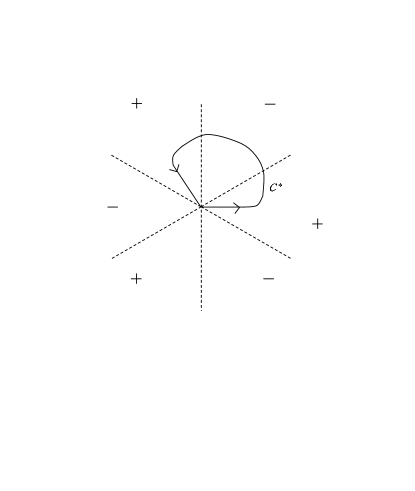
Figure 6. The contour ${\mathcal{C}}^{*}$ connects one positive sector to the next one.

One noteworthy fact is that the Stokes matrices depend on all terms in the connection, including regular terms. Thus, if $h(z)=\sum_{k=0}^{N}a_{k}z^{k}$, then $w$ in general depends on all coefficients $a_{k}$, including those with $k\geq n-1$. The Stokes matrices thus cannot be computed knowing only the singular part of the connection.

For a second example, we consider the Airy equation

(A.9) $$\left(\frac{d^{2}}{dx^{2}}+x\right)\Psi=0.$$

This equation is equivalent to

(A.10) $$\left(\frac{d}{dx}+\begin{pmatrix}0&-1\\ x&0\end{pmatrix}\right)\begin{pmatrix}u\\ v\end{pmatrix}=0,$$

with $u=\Psi$, $v=d\Psi/dx$. This equation has an irregular singularity at $x=\infty$; if we make the change of variables $z=1/x$, we get a differential equation with a singularity at $z=0$ that is of the type considered in eqn. (6.7), with $n=2$.

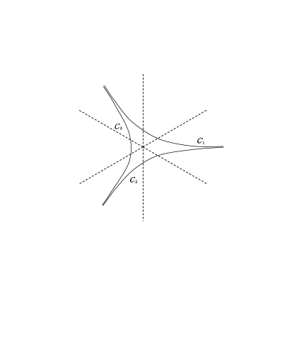
Figure 7. The contours ${\mathcal{C}}_{i}$ begin at infinity in the $i^{th}$ positive sector and end at infinity in the $i+1^{th}$. Their sum is homologous to zero.

This particular example of a differential equation with irregular singularity can be analyzed rather explicitly. Indeed, Airy’s equation can be solved by

(A.11) $$\Psi=\int_{\mathcal{C}}dp\,\exp(-p^{3}/3-px),$$

where ${\mathcal{C}}$ is a suitable contour. As the function being integrated is an entire function on the complex $p$-plane, there are no suitable closed contours. We must select a contour that begins and ends at infinity. There are three angular sectors in the $p$-plane in which ${\rm Re}\,p^{3}>0$. ${\mathcal{C}}$ must begin and end at infinity in one of these contours. If we denote as ${\mathcal{C}}_{i}$ a contour beginning in the $i^{th}$ positive sector and ending in the $i+1^{th}$ (fig. 7), then we get three solutions of Airy’s equations, namely

(A.12) $$\Psi_{i}=\int_{\mathcal{C}_{i}}dp\,\exp(-p^{3}/3-px),$$

But they obey $\Psi_{1}+\Psi_{2}+\Psi_{3}=0$, since ${\mathcal{C}}_{1}+{\mathcal{C}}_{2}+{\mathcal{C}}_{3}$ is a closed contour with no singularities inside.

To determine the asymptotic behavior of the solutions near the irregular singularity, that is for $x\to\infty$, we first note that the function $f(p)=p^{3}/3+px$ that appears in the exponent has two critical points, at

(A.13) $$p_{\pm}=\pm\sqrt{-x}.$$

Naively, the contribution of the critical point $p_{\pm}$ to the integral will be of order $\exp(\pm(2/3)(-x)^{3/2})$ (times an asymptotic series in negative powers of $x$). We expect each of the solutions $\Psi_{i}$ to have an asymptotic behavior for $x\to\infty$ that will be a linear combination of such exponentials. The Stokes phenomena mean, in this context, that the coefficients in these linear combinations will change when we cross certain lines.

A simple way to proceed is actually (as in the appendix to [31]) to start with a given critical point, say $p_{+}$, and ask what integral it dominates. We look for a steepest descent contour ${\mathcal{C}}_{+}$ through $p_{+}$ with the following properties: along ${\mathcal{C}}_{+}$, ${\rm Im}\,f$ is constant, and ${\rm Re}\,f$ is minimized at $p_{+}$. Because $f^{\prime}(p_{+})=0$ and $f^{\prime\prime}(p_{+})\not=0$, these conditions uniquely determine what ${\mathcal{C}}_{+}$ should look like near $p_{+}$. Requiring the right behavior near $p_{+}$ and imposing the condition that ${\rm Im}\,f$ is constant, we get a unique contour $\mathcal{C}_{+}$ which passes through $p_{+}$. Generically, it cannot be a closed contour; if it is closed, then ${\rm Re}\,f$ has a minimum on $\mathcal{C}_{+}$, which would be at a critical point of $f$. The only critical point other than $p_{+}$ is $p_{-}$; but generically ${\rm Im}\,f(p_{+})\not={\rm Im}\,f(p_{-})$ and a contour $\mathcal{C}_{+}$ passing through $p_{+}$ and with ${\rm Im}\,f$ constant cannot pass through $p_{-}$. So the contour $\mathcal{C}_{+}$ generically extends to infinity and connects two of the regions at infinity with ${\rm Re}\,p^{3}>0$. (It cannot start and end in the same region, since then the integral would vanish, while instead we will see momentarily that it is dominated by a single critical point.) Hence $\mathcal{C}_{+}$ is equivalent to one of $\mathcal{C}_{1},$ $\mathcal{C}_{2}$, or $\mathcal{C}_{3}$ (with one orientation or the other). The function that must be integrated over $\mathcal{C}_{+}$ has a constant phase and a maximum at $p_{+}$, so it is dominated for large $x$ by the contribution of $p_{+}$. So, as long as ${\rm Im}\,f(p_{+})\not={\rm Im}\,f(p_{-})$, one of the three solutions $\Psi_{1}$, $\Psi_{2}$, and $\Psi_{3}$ is asymptotic to $\exp((2/3)(-x)^{3/2})$. Similarly, one of the three solutions is dominated by the critical point $p_{-}$ and is asymptotic to $\exp(-(2/3)(-x)^{3/2})$.

Under $x\to\omega x$ with $\omega^{3}=1$, the three contours $\mathcal{C}_{i}$ and three solutions $\Psi_{i}$ are permuted. So there is no natural way to pair up two of them with the two critical points while omitting the third. The association of critical points $p_{\pm}$ with contours $\mathcal{C}_{i}$ changes in crossing the Stokes lines with ${\rm Im}\,f(p_{+})={\rm Im}\,f(p_{-})$, where our analysis of the behavior of $\mathcal{C}_{+}$ breaks down. By analyzing this process, one can compute the Stokes matrices explicitly.

For more on this, see the appendix to [31]. For much more on Airy’s equation, along with other examples, see [36].

References

- [1] M. F. Atiyah and R. Bott, “The Yang-Mills Equations Over Riemann Surfaces,” Phil. Trans. R. Soc. London 308 (1982) 523-615.
- [2] W. Balser, W. B. Jurkat, and D. A. Lutz, “Birkhoff Invariants And Stoke’s Multipliers for Meromorphic Linear Differential Equations,” J. Math. Anal. Appl. 71 (1979) 48-94.
- [3] A. Beauville, “Jacobiennes des Courbes Spectral et Systèmes Hamiltoniens Complètement Intégrables,” Acta Math. 164 (1990) 211-35.
- [4] A. Beilinson and V. Drinfeld, “Quantization Of Hitchin’s Integrable System And Hecke Eigensheaves,” preprint (ca. 1995), http://www.math.uchicago.edu/ arinkin/langlands/.
- [5] M. Bershadsky, A. Johansen, V. Sadov, and C. Vafa, “Topological Reduction Of SYM To Sigma Models,” Nucl. Phys. B448 (1995) 166-186, hep-th/9501096.
- [6] R. Bezrukavnikov, “Noncommutative Counterparts Of The Springer Resolution,” math.RT/0604445.
- [7] O. Biquard, “Fibrés de Higgs et connexions intégrables (diviseur lisse),” Ann. Sci. École Norm. Sup. (4), (1997) 30(1):41-96.
- [8] O. Biquard and P. Boalch, “Wild Non-Abelian Hodge Theory On Curves,” Compos. Math. 140 (2004) 179-204.
- [9] P. Boalch, “Symplectic Manifolds And Isomonodromic Deformations,” Adv. Math. 163 (2001) 137-205.
- [10] P. Boalch, “-Bundles, Isomonodromy, and Quantum Weyl Groups,” Int. Math. Res. Not. (2002) 1129-1166, math.DG/0108152.
- [11] P. Boalch, “Quasi-Hamiltonian Geometry Of Meromorphic Connections,” math.DG/0203161.
- [12] K. Corlette, “Flat -Bundles With Canonical Metrics,” J. Diff. Geom. 28 (1988) 361-82.
- [13] R. Donagi and E. Markman, “Spectral Curves, Algebraically Completely Integrable Hamiltonian Systems, And Moduli Of Bundles,” in Lecture Notes in Math. vol. 1620 (Springer, 1996) pp. 1-119, alg-geom/9507017.
- [14] R. Donagi and T. Pantev, “Langlands Duality For Hitchin Systems,” math/0604617.
- [15] E. Frenkel and D. Gaitsgory, “Local Geometric Langlands Correspondence And Affine Kac-Moody Algebras,” math.RT/0508382.
- [16] E. Frenkel, “Ramifications Of The Geometric Langlands Program,” math/0611294.
- [17] J. Gomis and S. Matsuura, “Bubbling Surface Operators And -Duality,” arXiv:0704.1657 [hep-th].
- [18] S. Gukov and E. Witten, “Gauge Theory, Ramification, And The Geometric Langlands Program,” hep-th/0612073.
- [19] J. A. Harvey, G. W. Moore, and A. Strominger, “Reducing Duality To Duality,” Phys. Rev. D52 (1995) 7161-7167.
- [20] T. Hausel and M. Thaddeus, “Mirror Symmetry, Langlands Duality, And The Hitchin System,” math.AG/0205236.
- [21] N. Hitchin, “The Self-Duality Equations On A Riemann Surface,” Proc. London Math. Soc. (3) 55 (1987) 59-126.
- [22] N. Hitchin, “Stable Bundles And Integrable Systems,” Duke Math. J. 54 (1987) 91-114.
- [23] N. Hitchin, “Geometrical Aspects Of Schlesinger’s Equation,” J. Geom. Phys. 23 (1997) 287-300.
- [24] N. Hitchin, “Langlands Duality And Spectral Curves,” math.AG/0611524.
- [25] M. Jimbo, T. Miwa, and K. Ueno, “Monodromy Preserving Deformations Of Linear Differential Equations With Rational Coefficients I,” Physica 2D (1981) 407-448.
- [26] A. Kapustin and E. Witten, “Electric-Magnetic Duality And The Geometric Langlands Program,” hep-th/0604151.
- [27] H. Konno, “Construction Of The Moduli Space Of Stable Parabolic Higgs Bundles On A Riemann Surface,” J. Math. Soc. Japan 45 (1993) 253-276.
- [28] I. Krichever, “The Isomonodromy Equations On Algebraic Curves, Canonical Transformations, and Whitham Equations,” hep-th/0112096.
- [29] B. Malgrange, “Sur les Déformations Isomonodromiques. I. Singularités Régulières,” Progr. Math. 37 (Birkh user, Boston, 1983).
- [30] G. Moore, “Geometry Of The String Equations,” Commun. Math. Phys. 133 (1990) 261-304.
- [31] J. Maldacena, G. Moore, and N. Seiberg, “Exact Vs. Semiclassical Target Space Of The Minimal String,” JHEP 0410:020 (2004), hep-th/0408039.
- [32] C. Sabbah, “Harmonic Metrics And Connections With Irregular Singularities,” Ann. Inst. Fourier (Grenoble) 49 (1999) 1265-1291, math.AG/9905039.
- [33] Y. Sibuya, “Linear Differential Equations In The Complex Domain: Problems Of Analytic Continuation” (Kinokuniya, Tokyo, 1976).
- [34] C. Simpson, “Harmonic Bundles On Noncompact Curves,” J. Am. Math. Soc. 3 (1990) 713-770.
- [35] A. Strominger, S.-T. Yau, and E. Zaslow, “Mirror Symmetry Is -Duality,” Nucl. Phys. B479 (1996) 243-259, hep-th/9606040.
- [36] W. Wasow, Asymptotic Expansions For Ordinary Differential Equations (Wiley, New York, 1965).
- [37] N. Woodhouse, “The Symplectic And Twistor Geometry of The General Isomondromic Deformation Problem,” nlin.SI/0007024.