A Multiresolution Census Algorithm for Calculating Vortex Statistics in Turbulent Flows

The fundamental equations that model turbulent flow do not provide much insight into the size and shape of observed turbulent structures. We investigate the efficient and accurate representation of structures in two-dimensional turbulence by applying statistical models directly to the simulated vorticity field. Rather than extract the coherent portion of the image from the background variation, as in the classical signal-plus-noise model, we present a model for individual vortices using the non-decimated discrete wavelet transform. A template image, supplied by the user, provides the features to be extracted from the vorticity field. By transforming the vortex template into the wavelet domain, specific characteristics present in the template, such as size and symmetry, are broken down into components associated with spatial frequencies. Multivariate multiple linear regression is used to fit the vortex template to the vorticity field in the wavelet domain. Since all levels of the template decomposition may be used to model each level in the field decomposition, the resulting model need not be identical to the template. Application to a vortex census algorithm that records quantities of interest (such as size, peak amplitude, circulation, etc.) as the vorticity field evolves is given. The multiresolution census algorithm extracts coherent structures of all shapes and sizes in simulated vorticity fields and is able to reproduce known physical scaling laws when processing a set of voriticity fields that evolve over time.

Key words. multivariate multiple linear regression, non-decimated discrete wavelet transform, penalized likelihood, turbulence, vorticity.

1 Introduction

The large-scale fluid motion of planetary atmospheres and oceans is extremely turbulent and is strongly influenced by the planetary rotation and the planet’s gravitational field. The planetary rotation and gravitation render the resulting fluid motion primarily horizontal. For example, in the Earth’s atmosphere, vertical motion is typically at speeds of several cm/s, while strong horizontal motions such as the jet stream can exceed speeds of 100 m/s. Turbulent fluids are characterized by having a wide range of spatial scales with complex non-linear interactions between the scales. One noteworthy feature of turbulent fluids is that they self-organize into coherent features. The two main categories of large-scale coherent structures are vortices; such as hurricanes, tornados, oceanic vortices, and Jupiter’s Great Red Spot, and jets; such as the Earth’s atmospheric Jet Stream, and the Gulf Stream in the North Atlantic Ocean. With respect to the scope of this manuscript we are only interested in identifying vortices, so the term coherent structure will be synonymous with vortex.

The reason for the formation of coherent structures is poorly understood. Due to the quasi-horizontal nature of atmospheres and oceans, the energy cascades from small to large scales, and the accumulation of energy at large scales is associated with large-scale coherent structures [McWilliams and WeissMcWilliams and Weiss1994]. Structures may also be formed from the growth of instabilities in the flow, with the scale of the structure determined by the scale of the instability. Regardless of their formation mechanism, accepting that such structures exist in turbulent flows and analyzing their behavior and impact has led to significant advances in understanding turbulence.

In many instances we wish to know the statistics of vortex properties. While traditional theories of turbulence are framed in terms of energy spectra, more recent theories are based around the statistics of the vortex population car-etal:evolution,mcc-wei:anisotropic. Coherent vortices in the ocean with spatial scales of tens of kilometers can live for more than a year and travel across the ocean, affecting the energetics, salinity, and biology of the ocean. The number and strength of such vortices is often determined by manually identifying vortices. One method of validating atmospheric models is determining whether they capture the statistics of atmospheric vortices such as storms and hurricanes. In all these areas, a robust efficient method to calculate the vortex statistics would represent a major advance.

Figure 1, which displays observations from a numerical simulation of turbulent flow, provides examples of such vortices. A vortex is a spinning, turbulent flow that possesses anomalously high (in absolute value) vorticity. Following the definition common for the Norther Hemisphere, positive vorticity (lighter shades in the images) corresponds to spinning in the counter-clockwise direction and negative vorticity (darker shades in the images) corresponds to spinning in a clockwise direction. Regions of high vorticity exhibit a peak near its center and decays back to zero vorticity in all directions from that center. The self-organization of a fluid into vortices is an emergent phenomena that can only be partially understood by analysis of the governing partial differential equations. Determining the details of a vortex population requires analyzing a time-evolved field, either from numerical simulations, laboratory experiments, or observations of natural systems, and requires a pattern recognition (or census) algorithm.

In order to determine the statistics of the vortices, one must first identify individual vortices and measure their properties. In two-dimensional turbulence the structure of the vortices is relatively simple and a broad variety of census algorithms have been successful [McWilliamsMcWilliams1990, Farge and PhilipovitchFarge and Philipovitch1993, Siegel and WeissSiegel and Weiss1997]. However one would like to develop methods of structure identification that work in more realistic fluid situations ranging from three-dimensional idealized planetary turbulence to the most realistic General Circulation Model (GCM). In these situations, the structures include jets as well as vortices, and these structures exist in a more complex fluctuating environment. The goal of the current work is to develop a census algorithm for identifying vortices in two-dimensional turbulence that is sufficiently general to handle, with modifications, these more realistic situations.

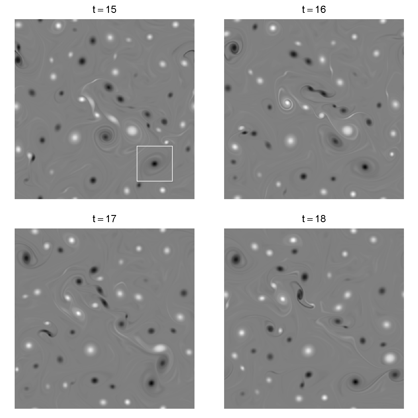
Figure 1: Observed vorticity fields ($512{\times}512$ pixels) from a numerical simulation at times $t\in\{15,16,17,18\}~{}\text{seconds}$. Negative vorticity is seen as darker shades of grey approaching black, while positive vorticity is seen as lighter shades of grey approaching white. The background, roughly zero vorticity, is a medium grey. The white square in the lower-right corner of the vorticity field at $t=15$ is centered at the largest coherent structure, in peak absolute vorticity.

The “data mining” of turbulent fluid flow, both simulated and observed, can be thought of as a statistical problem of feature extraction. In this work we focus on the detection of coherent structures from a simulated scalar field of rotational motion. The reason that we focus on simulated fields is that real data at the required resolution is difficult to obtain in practice. Our approach to this problem consists of two parts. The first step is to develop a flexible model for a single coherent “template” structure (vortex) using multiresolution analysis and the second identifies individual vortices through a stepwise model selection procedure. Although the model for the template function embodies prior information from the scientist, it is flexible enough to capture a broad range of features associated with coherent structures one might observe in fluid. Once a suitable template is chosen, the second step provides an objective approach to identifying features of interest through classic statistical methodology, allowing the information in the vorticity field to dictate what is and what is not a vortex. With individual coherent structures efficiently summarized through a set of parameters, such as diameters and centroid locations, the next step of modeling movement and vortex interaction may take place; e.g., sto-etal:asilomar. This has the potential to advance our understanding of many complex natural systems, such as hurricane formation and storm evolution.

In the past, coherent structures have been quantified by simply decomposing the flow into signal and background noise using wavelet-based techniques; see, for example, far-etal:improved, wic-etal:ecwpalc, wic-far-goi:tdcst and the summary article by far-etal:turbulence. The focus of the methodology used in these papers has a engineering orientation; that is, the wavelet transform is used to discriminate between signal and noise using compression rate as a classifier. The idea being that the coherent structures (vortices) observed in the turbulent flow will be well-represented by only a few wavelet coefficients and therefore most coefficients may be discarded. From one vorticity field, two fields are produced from such a procedure: one based on the largest wavelet coefficients that is meant to capture the largest coherent structures in the original field; and another, based on the remaining wavelet coefficients, is a mixture of background structures (i.e., filaments) and noise.

sie-wei:census developed a wavelet-based census algorithm for two-dimensional turbulence that relied on specific attributes of coherent structures. First, the vorticity field was separated into coherent and background fields using an iterative wavelet thresholding technique, then the surviving wavelet coefficients in the coherent part are grouped according to the spatial support of the Haar basis. luo-lel:eddies investigated a wavelet-based technique for identifying, labeling and tracking ocean vortices and a database was built of wavelet signatures based on the amount of energy contained at each scale. They found that Gaussian densities were adequate to model observed vortices.

Our methodology differs significantly from the signal-plus-noise model and other wavelet-based techniques. Our main scientific contribution is the development and efficient implementation of a statistical method to extract a wide variety of coherent structures from two-dimensional turbulent fluid flow. We achieve this through the formulation of a flexible statistical model for individual coherent structures (vortices) and obtain a fixed number of isolated vortices from the original field via regression methodology. From these models a completely different set of summary statistics may be calculated; for example, instead of global summary statistics like the enstrophy spectrum over the entire image we are able to look at local statistics for each structure such as the average size, amplitude, circulation and enstrophy of the individual vortices.

This work has lead to new models for two-dimensional multiscale features. Although this work concentrates on vortices, the proposed methodology is quite generic and can be transferred to model other types of coherent structures. The adaptation of model selection methods for segmenting images is made possible by formulating our model in terms of multiple linear regression. Finally, we note this work also depends on the development of computing algorithms whereby one fits many local regressions simultaneously using equivalences with image convolution filtering. The statistical computing aspects of this problem are important in order to analyze large problems that are of scientific interest. As a test of these ideas we are able to carry out a census of vortices from a high-resolution simulation of two-dimensional turbulence.

The next section provides a brief introduction to two-dimensional turbulence and the numerical simulation used. Section 3 outlines how we model individual coherent structures and the entire vorticity field. The two-dimensional multiresolution analysis approach to images is introduced and the user-defined vortex template function is also discussed. Section 4 provides the methodology to estimate a single coherent structure and also multiple structures in the vorticity field. Section 5 looks at how well the technique performs at estimating multiple coherent structures and at the temporal scaling of vortex statistics.

2 Two-dimensional Fluid Turbulence

Turbulence in atmospheres and oceans occur in many forms and at many scales. Two-dimensional turbulent flow is an idealization that captures many of the features of planetary turbulence, and in particular, has vortex behavior that is common to many atmospheric and oceanic phenomena. Thus, two-dimensional turbulence often serves as a laboratory to study aspects of planetary turbulence and as a testbed for developing theories and algorithms. Here we follow this strategy and use two-dimensional turbulence to develop and test a new multiresolution census algorithm for vortex statistics. While there are experimental fluid systems that approximate two-dimensional fluid flow, numerical simulations are the most effective way to develop and test such algorithms. Treating the output of numerical simulations as data which is analyzed just as one would with observations or laboratory experiments is routine in the field of turbulence and we follow this route.

Two dimensional fluid dynamics has a long history and many aspects are well understood [Kraichnan and MontgomeryKraichnan and Montgomery1980, FrischFrisch1995, LesieurLesieur1997]. The equations of motion for two-dimensional turbulence are written in terms of the fluid velocity $\vec{u}=(u_{x},u_{y})$, and its scalar vorticity

$$\zeta(\vec{u})=(\nabla\times\vec{u})\cdot\hat{z},$$

where $\nabla$ is the gradient operator and $\hat{z}$ is a unit vector in the direction perpendicular to the plane containing the two-dimensional velocity $\vec{u}$. In general the curl of a vector field is given by $\nabla\times\vec{u}$ and, hence, vorticity is the curl of the velocity field. Following the “right-hand rule” vorticity is positive when the flow is rotating anti-clockwise and negative otherwise. A related concept is circulation which is related to vorticity by Stoke’s theorem

$$\Gamma(\vec{u})=\int_{S}\zeta(\vec{u})\,\text{d}S,$$

where $S$ is a surface in two dimensions. The units of circulation are length squared over time and vorticity is the circulation per unit area. Enstrophy is given by

$$\mathcal{E}(\vec{u})=\frac{1}{A}\int_{S}|\zeta(\vec{u})|^{2}\,\text{d}S,$$

where $A$ is the area of the fluid, and is a measure of the mean-square vorticity. Enstrophy is a quantity that is similar to energy (which is the mean-square velocity) and plays an important role in turbulence theory despite being somewhat non-intuitive.

It is important to understand fluid flow at a macroscopic scale and, in particular, create more accurate models for the flow of the atmosphere and ocean. Recent advances in computing have allowed scientists to produce more realistic simulations of turbulent flows [FerzigerFerziger1996, Moin and MaheshMoin and Mahesh1998]. Numerical simulation of two-dimensional turbulence show that random initial conditions will self-organize into a collection of coherent vortices which subsequently dominate the dynamics (McWilliams mcw:emergence,mcw:vortices). Due to this self-organization, traditional scaling theories of turbulence fail to correctly describe the dynamics, while scaling theories based on the statistics of the vortices are much more successful car-etal:evolution,wei-mcw:temporal-scaling,bra-etal:revisiting.

2.1 Data description

The equations of motion for two-dimensional fluid flow are

$$\frac{\partial\zeta}{\partial t}+(\vec{u}\cdot\nabla)\zeta=\mathcal{D}\quad\text{and}\quad\zeta=(\nabla\times\vec{u})\cdot\hat{z},$$

where $\mathcal{D}$ is a general dissipation operator. Despite being small, dissipation is an important component of turbulence and is necessary for numerical simulations. Due to the nature of two-dimensional turbulence, energy cascades to large scales and is not dissipated in the limit of small dissipation, while enstrophy cascades to small scales and has finite dissipation in the limit of small dissipation. The dissipation of enstrophy is governed by the evolution of the vortex population. These equations are simulated with doubly periodic boundary conditions using a pseudo-spectral algorithm, using a hyperviscous diffusion operator $\mathcal{D}=-\nu\nabla^{4}\zeta$ on a $512{\times}512$ grid. The simulations start from small-scale random initial conditions.

As time proceeds, the random initial conditions self-organize into coherent vortices. The initial scale of the vortices is governed by the scale of the initial conditions. Subsequently, vortices grow through vortex mergers until a final end-state is reached with two vortices, one of each sign. During the time period after self-organization but before the vortex number gets too small, the turbulence can be modeled as a population of interacting coherent vortices. We emphasize that the vortices are not introduced into the flow by any external forcing, but rather they arise through the natural self-organizing nature of two-dimensional turbulence.

Here we apply our algorithm solely to data from numerical experiments. The equations of motion and the methods for solving them are firmly established and previous work in fluid dynamics has shown that numerical simulations, laboratory experiments, and observations of natural systems all produce vortices with similar properties. Numerical simulations provide the most complete and accurate representation of vortex dynamics and thus provide the most stringent test for the proposed algorithm.

3 Models for Vorticity Fields

The goal of our multiresolution census algorithm is to identify all coherent structures (vortices) from a given vorticity field and then compute summary statistics from each identified structure. As discussed in the introduction, this approach differs from previous ones in that we are not interested in merely separating the coherent portion of the field from the background, as in the traditional signal-plus-noise model, but instead isolate individual coherent structures in the image for further analysis. For the simple vortex fields considered here, our proposed method performs similarly to previous methods. This is quantitatively demonstrated by the scaling relations shown in Figure 8. However, previous methods are not easily extended to flows with more complex structure. The general statistical framework of the current approach provides a flexible modelling framework in which to implement generalizations in a relatively straightforward manner.

For clarity we first outline a continuous version of the problem and then follow by a more practical discrete approximation. Let $\zeta_{t}(\mathbf{x})$ denote an observed vorticity field at time $t$ and location $\mathbf{x}\in\mathbb{R}^{2}$. Given $S$ vortices, $\zeta_{t}(\mathbf{x})$ can be decomposed as

$$\zeta_{t}(\mathbf{x})=\sum_{s=1}^{S}v_{s}(\mathbf{x})+e_{t}(\mathbf{x})$$ (1)

where $v_{s}$ is the localized vorticity associated with each coherent structure and $e_{t}$ is the background variation from other types of structures. Given the dominance of vortices in our application, it is useful to assume a stochastic character for the residual component $e_{t}$. The statistical problem is: given the observed field $\zeta_{t}$, estimate $S$ and $\{v_{s}\}$.

The main modeling component in this work is to expand the individual vortex field in a finite basis

$$v_{s}=\sum_{i=1}^{M}\alpha_{s,i}z_{i}(\mathbf{x}-\boldsymbol{\mu}_{s})$$ (2)

where $\boldsymbol{\mu}_{s}$ approximates the center of the vortex and the (linear) coefficients $\{\alpha_{s,i}\}$ determine the shape. Estimation procedures for $\boldsymbol{\mu}_{s}$ and $\{\alpha_{s,i}\}$ are discussed in Section 4. The basis functions $\{z_{i}\}$ are designed to provide a multiscale representation of coherent structures and build in prior knowledge of the vortex shape. Their specification is motivated in the next two sections.

3.1 Multiresolution Analysis (MRA)

The use of wavelets for two-dimensional image analysis and compression has a large literature and at its heart is the decomposition of an image into different scales or levels of resolution [Vetterli and KovačevićVetterli and Kovačević1995, MallatMallat1998]. In our work we assume the scale to be in powers of two and within a scale consider a further decomposition that divides features into three orientations: vertical, horizontal, and diagonal. The net result is that for a given initial vorticity field $\zeta_{t}$ and $J$ levels of resolution ($J=6$ is used when applying the model in practice), we decompose the field into the sum of $(3J+1)$ distinct components: three different orientations for each level of resolution and a smoothed field. Heuristically, as the levels increase the main features at each level will increase in size by a factor of two. Strong horizontal features at a given scale are represented by the horizontal component while similar correspondences hold for the vertical and diagonal components. Later, it will be exploited that some of these level-specific features may correspond to features at (possibly different) levels of the decomposition of the vorticity field.

We assume that the vorticity field $\zeta(\mathbf{x})$ has finite energy; i.e., $\int_{\mathbf{x}}\zeta^{2}(\mathbf{x})<\infty$ and let $\phi$ be a scaling function and $\psi$ be the corresponding wavelet generating an orthonormal basis on $L^{2}(\mathbb{R})$. Define the three separable two-dimensional wavelets

$$\psi^{\text{h}}(x_{1},x_{2})=\phi(x_{1})\psi(x_{2}),\quad\psi^{\text{v}}(x_{1},x_{2})=\psi(x_{1})\phi(x_{2}),\quad\psi^{\text{d}}(x_{1},x_{2})=\psi(x_{1})\psi(x_{2}),$$

corresponding to the horizontal, vertical, and diagonal directions, respectively. This follows from the fact that the two-dimensional wavelets are the outer product of two one-dimensional wavelet and scaling functions, where the scaling function averages (smooths) across its spatial direction while the wavelet function differences across its spatial direction. The two-dimensional wavelet $\psi^{\text{h}}(x_{1},x_{2})=\phi(x_{1})\psi(x_{2})$ will therefore smooth across the first dimension ($x_{1}$-axis) and difference across the second dimension ($x_{2}$-axis), thus favoring horizontal features. The two-dimensional wavelet basis function $\psi^{\text{v}}(x_{1},x_{2})=\psi(x_{1})\phi(x_{2})$ differences across the $x_{1}$-axis and smooths across the $x_{2}$-axis, thus favoring vertical features and $\psi^{\text{d}}(x_{1},x_{2})=\psi(x_{1})\psi(x_{2})$ differences across both directions and favors non-vertical/non-horizontal (i.e., diagonal) features. The separable scaling function $\phi(x_{1},x_{2})=\phi(x_{1})\phi(x_{2})$ is associated with the approximation space.

Although the 2D DWT, as a decimated orthonormal transform, would be a more efficient representation of the vorticity field we find it advantageous to utilize the 2D maximal overlap DWT (2D MODWT). Unlike the orthonormal transform, the 2D MODWT produces a redundant non-orthogonal transform. The reason for this discrepancy is that the 2D MODWT does not subsample in either dimension, it only filters the original image. The advantages are that the transform is translation invariant to integer shifts in space and it reduces potential artifacts caused by how the wavelet filter represents abrupt changes in the image.

Assume both $\psi$ and $\phi$ have been rescaled so that the squared norm of the wavelet coefficients equals the squared norm of the original observations. The separable wavelet functions associated with specific scale and spatial directions $D\in\{\text{h},\text{v},\text{d}\}$ are given by

$$\psi_{j,k,l}^{D}(x_{1},x_{2})=\frac{1}{2^{2j}}\psi^{D}\left(\frac{x_{1}-k}{2^{j}},\frac{x_{2}-l}{2^{j}}\right),\quad j=1,\ldots,J,\quad k=1,\ldots,M,\quad l=1,\ldots,N.$$

The separable scaling function $\phi_{j,k,l}$ is defined similarly. Hence, each level in the transform will have the same spatial dimension as the original field $(M\times{N})$ and represent a redundant set of wavelet coefficients. The 2D MODWT begins with the original vorticity field $\zeta$ (the spatial location will be omitted when implied), and at all scales we denote $\omega_{j}^{\phi}=\langle{\zeta,\phi_{j,k,l}}\rangle$ and $\omega_{j}^{D}=\langle{\zeta,\psi_{j,k,l}^{D}}\rangle$ for $D\in\{\text{h},\text{v},\text{d}\}$, where $\langle{x,y}\rangle$ is the two-dimensional inner product. The vorticity field $\zeta(\mathbf{x})$ may now be decomposed into $3J+1$ sub-fields: three fields of wavelet coefficients at each resolution level corresponding to distinct spatial directions and one field containing the scaling coefficients at the final level. The scaling (approximation) field for level $j$ may be obtained from the four fields at level $j+1$ via

$$\omega_{j}^{\phi}(\mathbf{x})=\left\{\omega_{j+1}^{\phi}*\phi_{j,k,l}\right\}+\sum_{D}\left\{\omega_{j+1}^{D}*\psi_{j,k,l}^{D}\right\},$$ (3)

where “$*$” denotes the convolution operator.

The two-dimensional multiresolution analysis (MRA) of the vorticity field is an additive decomposition given by recursively applying (3) over all $j$; i.e.,

$$\zeta(\mathbf{x})=\left\{\omega_{J}^{\phi}*\phi_{J,k,l}\right\}+\sum_{j=1}^{J}\sum_{D}\left\{\omega_{j}^{D}*\psi_{j,k,l}^{D}\right\}=\alpha_{J}^{\phi}(\mathbf{x})+\sum_{j=1}^{J}\sum_{D}\alpha_{j}^{D}(\mathbf{x}),$$

where $\alpha_{J}^{\phi}$ is the wavelet approximation field and $\alpha_{j}^{D}$ is the wavelet detail field associated with the spatial direction $D\in\{\text{h},\text{v},\text{d}\}$. The MRA of $\zeta(\mathbf{x})$ provides a convenient way of isolating features at different scales and directions with coefficients in the spatial domain versus the wavelet domain. This is advantageous since reconstruction is now reduced from the full inverse 2D MODWT to simple addition and potential phase adjustments are eliminated.

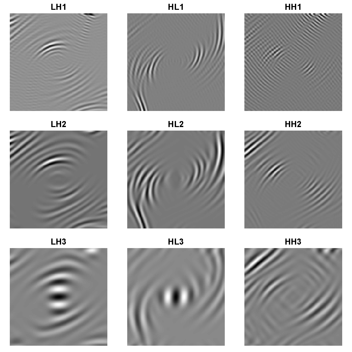
Figure 2: Two-dimensional multiresolution analysis $(j=1,2,3)$ of a $100{\times}100$ pixel section of the vorticity field centered at $(x,y)=(399,101)$ using the Daubechies least asymmetric wavelet filter $(L=8)$. LH corresponds with horizontal, HL with vertical and HH with diagonal wavelet coefficients. This pixel section is the area highlighted by the white square box in the top left panel of Figure 1.

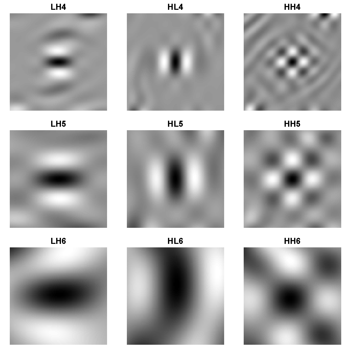
Figure 3: Two-dimensional multiresolution analysis $(j=4,5,6)$ of a $100{\times}100$ pixel section of the vorticity field centered at $(x,y)=(399,101)$ using the Daubechies least asymmetric wavelet filter $(L=8)$. LH corresponds with horizontal, HL with vertical and HH with diagonal wavelet coefficients.

Figures 2 and 3 display the six scales from a two-dimensional MRA of the sample vorticity field in Figure 1 (at $t=15$), defined by a $100{\times}100$ pixel section centered at $(x,y)=(399,101)$. Each row displays the wavelet detail fields associated with the three spatial directions: horizontal, vertical and diagonal. It is clear that each of the two-dimensional wavelet filters captures distinct spatial directions at a fixed spatial scale. Given the filaments from this particular vortex are elliptical in shape, it is not surprising to see the detail coefficients of the filament structures strongest in the northeast-southwest directions. It is interesting to note that the coherent structure (i.e., the dark region in the center of the image) is not seen until the third scale (third row in Figure 2) and then only in the horizontal and vertical directions. At higher scales, corresponding to larger spatial areas and lower spatial frequencies, the coherent structure is apparent in all three directions. This is most likely due to the spatial extent (size) of the structure at time $t=15$ in the simulation.

3.2 Single Vortex Model

Recall that a vortex may be loosely described as a concentration of anomalously high (in absolute value) vorticity. As a simple outline of a vortex we consider the Gaussian kernel. If we translate a single vortex to the origin, then $\tau(\mathbf{x})=\eta\exp(-\left\|\mathbf{x}\right\|^{2}/\sigma^{2})$ is our vortex template function where $\eta$ is the maximum vorticity at its center. This choice for $\tau(\mathbf{x})$ visually appears to capture the relevant features of an idealized vortex even when the observed vortices decay back to zero at a different rate than Gaussian tails. For illustration in Figure 4, $\eta$ and $\sigma^{2}$ were chosen to coincide with the peak value and spread of the specific coherent structure. However, when used in the multiresolution census algorithm the template function will have a fixed magnitude and spread – any modifications to fit the vortex will be induced by the multiscale representation of $\tau(\mathbf{x})$. Thus, a perfect fit is not required since deviations from Gaussianity will be captured through the model fitting procedure.

Figure 4: Vortex cross sections (solid line) and normalized Gaussian kernels (dashed line) from the observed vorticity field at time $t=15$.

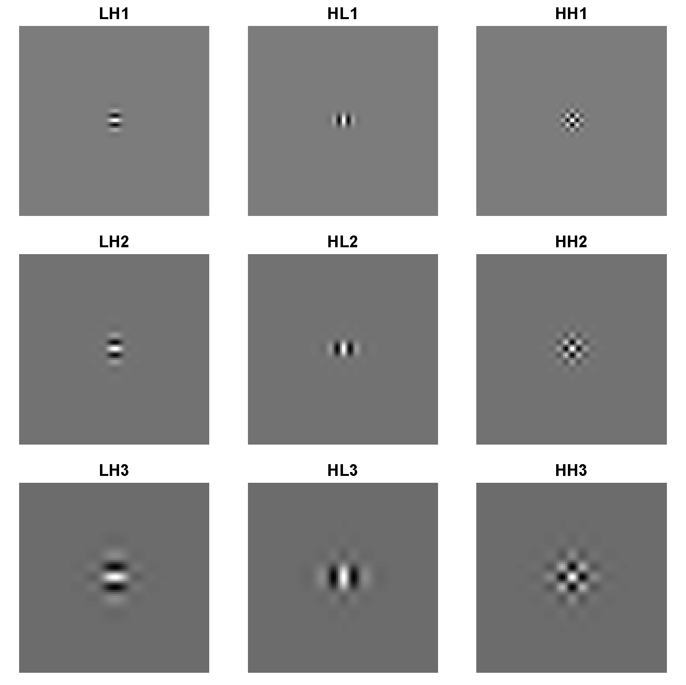
Figure 5: Two-dimensional multiresolution analysis $(j=1,2,3)$ of a $100{\times}100$ pixel section of the template function. The rows correspond to the scale $j$ and the columns correspond to spatial directions: LH is horizontal, HL is vertical and HH is diagonal.

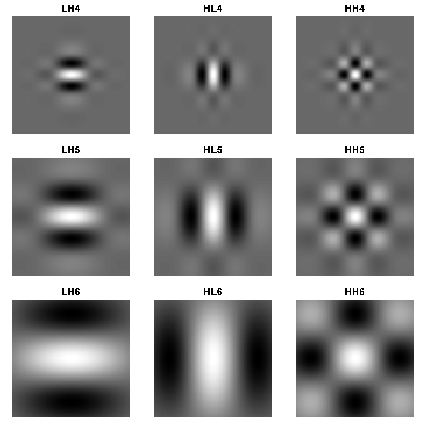
Figure 6: Two-dimensional multiresolution analysis $(j=4,5,6)$ of a $100{\times}100$ pixel section of the template function. The rows correspond to the scale $j$ and the columns correspond to spatial directions: LH is horizontal, HL is vertical and HH is diagonal.

Figures 5 and 6 show an MRA $(J=6)$ of $\tau(\mathbf{x})$ derived from the outer product of two zero-mean Gaussian kernels with the same variance. The rows correspond to wavelet scales and the columns correspond to spatial directions within each scale. Although the Gaussian kernel is too simple for modeling an observed vortex directly, the components of its MRA are strikingly similar to the MRA of individual coherent structures in the observed vorticity field (Figures 2 and 3). This observation identifies the basic components for building a template basis and is key to our methodology. We propose to represent each matrix of vorticity coefficients as a linear combination of the matrices derived from the MRA of the Gaussian kernel. A straightforward way to relate the MRA of an observed coherent structure to the template function is through a series of simple linear regression models relating the multiresolution coefficients from the observed vorticity field $\boldsymbol{\alpha}$ with the multiresolution coefficients from the template function $\mathbf{z}$ via

$$\begin{array}[]{lcll}\alpha_{j,k,l}^{D}&=&\beta_{j}^{D}z_{j,k,l}^{D}+\epsilon_{j,k,l}^{D},&\quad k=1,\ldots,M,\quad l=1,\ldots,N;~{}\text{for all $j,D$}\\ \alpha_{J,k,l}^{\phi}&=&\xi_{J}^{\phi}+\beta_{J}^{\phi}z_{J,k,l}^{\phi}+\epsilon_{J,k,l}^{\phi},&\quad k=1,\ldots,M,\quad l=1,\ldots,N.\end{array}$$ (4)

At each spatial scale and direction there is only one final parameter to be fit, since each image from the MRA is guaranteed to be mean zero except for the smoothed field $\boldsymbol{\alpha}^{\phi}$. The implied linear relation between the multiresolution components of the data and template function allows for differences in the magnitude and direction of vorticity through the regression coefficients. That is, once $\tau(\mathbf{x})$ is defined (using fixed parameters $\eta$ and $\sigma^{2}$) we will use it to model all possible coherent structures in the vorticity field. The MRA decomposes the template function into spatial scales and directions, but the model in Equation (4) is limited because each spatial scale and direction from $\zeta(\mathbf{x})$ is tied to the same spatial scale and direction of $\tau(\mathbf{x})$. To make full use of the MRA, we propose to estimate every spatial scale and direction of the observed vorticity field using all possible spatial scales and directions from the template function. This suggests the following multiple linear regression model:

$$\alpha_{j,k,l}^{D}=\beta_{1}^{\text{h}}z_{1,k,l}^{\text{h}}+\beta_{1}^{\text{v}}z_{1,k,l}^{\text{v}}+\beta_{1}^{\text{d}}z_{1,k,l}^{\text{d}}+\cdots+\beta_{J}^{\text{h}}z_{J,k,l}^{\text{h}}+\beta_{J}^{\text{v}}z_{J,k,l}^{\text{v}}+\beta_{J}^{\text{d}}z_{J,k,l}^{\text{d}}+\beta_{J}^{\phi}z_{J,k,l}^{\phi}+\epsilon_{j,k,l}^{D},$$ (5)

$k=1,\ldots,M,l=1,\ldots,N$; for all $j,D$. The linear regression model for the field of wavelet smooth coefficients in Equation (4) does not change. The intercept is included to account for potential low-frequency oscillations that may not be provided by the template function. At each spatial scale and direction from the observed vorticity field there are $(3J+1)$ parameters to be fit. The full multivariate multiple linear regression model for a single vortex may now be formulated as

$$\mathbf{Y}=\mathbf{Z}\boldsymbol{\beta}+\boldsymbol{\epsilon},$$ (6)

where $\mathbf{Y}$ is the $MN{\times}(3J+1)$ response matrix from the MRA of the observed vorticity field, $\mathbf{Z}$ is the $MN{\times}(3J+1)$ design matrix whose columns consist of the MRA of the template function centered at the location $\boldsymbol{\mu}$, and $\boldsymbol{\beta}$ is the $(3J+1)\times(3J+1)$ regression coefficient matrix a given coherent structure.

There are several differences between the Gaussian kernel $\tau(\mathbf{x})$ and the observed vorticity field $\zeta(\mathbf{x})$ that are handled automatically through the multivariate multiple linear regression model in Equation (5), these include: fixed spatial size, amplitude, and radial symmetry. The fixed spatial size of $\tau(\mathbf{x})$ is taken care of by the fact that all spatial scales from its MRA are associated with each spatial scale in the observed vorticity field. The scale dependent multiple linear regression, Equation (5), may represent any particular spatial scale of $\zeta(\mathbf{x})$ and associate it with any spatial scale of $\tau(\mathbf{x})$. Thus, larger spatial scales may be either favored or penalized through the individual regression coefficients. The amplitude of the template function is similarly handled through the magnitude of these regression coefficients.

An initial impression may be that the radial symmetry of $\tau(\mathbf{x})$ will restrict the model to radially symmetric vortices. However, asymmetry is accommodated through the multivariate multiple linear regression by decoupling the three unique spatial directions. Each spatial direction is manipulated through its own regression coefficient, thus allowing for eccentric vortex shapes by favoring one or two of the three possible spatial directions at each scale (Figures 5 and 6).

The level of association needed between the template function and feature of interest in order to model the vorticity field is currently unknown. We have found that small pixel shapes, such as a Gaussian or triangular function, work well in the problem presented here. However, we believe this algorithm is quite adaptive through the user-defined template function $\tau(\mathbf{x})$. For example, if the filament structures were deemed interesting in this problem, an effective template function to pick out these features could consist of nothing more than a collection of concentric circles.

4 Model Estimation

4.1 A Linear Model Framework

Based on the previous development of the template function and the final step of discretization we are led to the following model for a vortex field at a single time point:

$$\mathbf{Y}=\mathbf{Z}_{1}\boldsymbol{\beta}_{1}+\mathbf{Z}_{2}\boldsymbol{\beta}_{2}+\cdots+\mathbf{Z}_{S}\boldsymbol{\beta}_{S}+\boldsymbol{\epsilon},$$ (7)

where $\mathbf{Y}$ is the $MN{\times}(3J+1)$ response matrix from the MRA of the observed vorticity field (the columns index the spatial scales and direction where each column vector is the result of unwrapping the $M{\times}N$ image matrix into a vector of length $MN$), $\mathbf{Z}_{s}$ is the $MN{\times}(3J+1)$ design matrix whose columns consist of the MRA of the template function centered at the location $\boldsymbol{\mu}_{s}$, and $\boldsymbol{\beta}_{s}$ is the $(3J+1)\times(3J+1)$ regression coefficient matrix for the $k$th coherent structure. Note that this model parallels the continuous versions in Equations (1) and (2), but for fixed $S$ and $\{\boldsymbol{\mu}_{s}\}$ is a linear model. Given this framework, the main statistical challenge is model selection, determining the number of coherent structures $S$, and their locations $\{\boldsymbol{\mu}_{s}\}$.

4.2 Coherent Feature Extraction

We choose to implement our procedure for coherent structure extraction in a modular fashion so that we may modify specific steps without jeopardizing the integrity of the entire method. To this end, the first major step is to produce a set of vortex candidate points $\mathcal{C}$ (coordinates in two dimensions); that is, a subset of all possible spatial locations in the observed vorticity field. Our goal at this point is not to generate the exact locations of all coherent structures in the field, but we want $\mathcal{C}$ to contain all possible coherent structures and additional spatial locations that are not vortices; i.e., $MN\gg\#\mathcal{C}>S$. Although the number of elements in $\mathcal{C}$ is large, their refinement is amenable to more conventional statistical analysis. Vortices are selected from $\mathcal{C}$ using classic likelihood procedures to obtain a final model. The first step is a rough screening of the model space and should be done with computational efficiency in mind. The second step devotes more computing resources on a much smaller set of models.

4.2.1 Candidate Point Selection

Instead of relying on specific features in the vorticity field that are present in our current data set and may or may not be present in future applications, we propose a model-based approach to extracting the set of vortex candidate points $\mathcal{C}$. After selecting an appropriate template function $\tau(\mathbf{x})$, we fit a single-vortex model (Section 3.2) to every $M{\times}N$ spatial locations. This is done in a computationally efficient manner by first performing an orthogonal decomposition on the design matrix $\mathbf{Z}$ and using a discrete Fourier transform to perform the matrix multiplications whi-etal:stochastic. The result is that the multivariate multiple linear regression model in Equation (7) can be fit to all $M{\times}N$ grid points in the image without the need for a massive computing environment. The reason for fitting the single-vortex model everywhere is that we may now use the regression coefficient matrix $\hat{\boldsymbol{\beta}}_{s}$ to indicate the presence or absence of a coherent structure at $\boldsymbol{\mu}_{s}$. This technique has the inherent flexibility of the template function. If a different feature was to be extracted from the vorticity field, we would simply fit a different template function and use its regression coefficients.

With a regression coefficient matrix for each location, a distance measure is computed between $\hat{\boldsymbol{\beta}}$ and the identity matrix $\mathbf{I}_{J}$, of dimension $(3J+1)$, using

$$\Lambda=\min\left\{\text{tr}\left[(\hat{\boldsymbol{\beta}}-\mathbf{I}_{J})^{2}\right],\text{tr}\left[(\hat{\boldsymbol{\beta}}+\mathbf{I}_{J})^{2}\right]\right\}.$$

The idea is that $\Lambda$ measures the feasibility that a vortex is centered at this location. The value of $\Lambda$ is small when the regression matrix $\hat{\boldsymbol{\beta}}$ is similar to the identity matrix, and thus, the single-vortex model is similar to the template function. Two comparisons are made, one to the positive identity matrix and one to the negative identity matrix, so that positive and negative spinning vortices are favored equally. The parametric image of $\Lambda$ values is smoothed using a nine-point nearest-neighbor kernel with weights based on Euclidean distance. A local minimum search is performed on the smoothed image in order to obtain the set of candidate points $\mathcal{C}$. We found that this technique captures all coherent structures one can identify visually in the vorticity field along with additional features that may or may not be vortices.

4.2.2 Model Selection for the Vortex Field

A final selection of coherent structures from the set of candidate points $\mathcal{C}$ is achieved through forward subset selection by minimizing the generalized cross-validation (GCV) function

$$\text{GCV}(S)=\frac{\text{RSS}(S)/(MN)}{[1-p(S)/(MN)]^{2}},$$

for a given choice of $S$ vortex locations. Here $\text{RSS}(S)$ is the residual sum of squares and $p(S)$ is the total number of effective parameters in Equation (7). The following simple method was adopted to count the total number of effective parameters. For each estimated $\boldsymbol{\beta}_{s}$ in Equation (7), denoted as $\hat{\boldsymbol{\beta}}_{s}=(\hat{\beta}_{1},\ldots,\hat{\beta}_{(3J+1)\times(3J+1)})$, its effective number of parameters is defined as the number of $\hat{\beta}_{j}$’s whose absolute value is greater than twice the sample standard deviation of the $\hat{\beta}_{j}$’s. Then the overall total effective number of parameters in Equation (7) is calculated as the sum of the effective number of parameters of $\hat{\boldsymbol{\beta}}_{s}$ for all $s$.

Because of the size of this problem, it is not possible to compute $\hat{\boldsymbol{\beta}}$ via exact linear algebra. For an observed vorticity field with $M=N=512$ and $J=6$, model fitting will produce approximately 95 million regression coefficients. Instead we use an iterative method, backfitting [Friedman and StuetzleFriedman and Stuetzle1981], to find an approximate solution to the $S(3J+1)^{2}$ simultaneous linear equations associated with Equation (7). Convergence for this algorithm is achieved by looking at the absolute difference between each regression coefficient matrix $\hat{\boldsymbol{\beta}}$ from step $i-1$ to $i$. The number of iterations was found to be small across a wide range of $S$, usually two to four iterations sufficed. We attribute the small number of iterations to the fact that most coherent structures in $\zeta(\mathbf{x})$ are spatially isolated; see, e.g., Figure 1.

5 Application to Two-dimensional Turbulent Flows

Now we return to the simulated vorticity field in Figure 1 and compute the vortex statistics using our multiresolution census algorithm outlined in Section 4.2.

5.1 Isolated and Multiple Coherent Structures

The vorticity field at time step $t=15$ from the numerical simulation provides a reasonable example of multiple coherent structures embedded within a quiescent background. Summary statistics for this vorticity field include an average circulation given by $\bar{\zeta}=384.10$, an average enstrophy of $\bar{\mathcal{E}}=397.4{\times}10^{3}$, and an average maximum peak amplitude of 25.63.

To illustrate the ability of our procedure to find coherent structures of varying sizes and shapes, Figure 7 shows the results from the two stages of our census algorithm: coherent structures identified from our candidate procedure, the fitted vortex field model and the residual field ($t=15$). The set of candidate points, roughly 200, appears to capture all potential vortices apparent through visual inspection along with other locations that do not appear to contain a substantial accumulation of vorticity. After model selection, a total number of 54 coherent structures were identified. Although the template function has fixed spatial size and amplitude, the fitted coherent structures are distinct from it and from each other, and exhibit a wide variation in both size and amplitude.

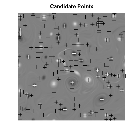
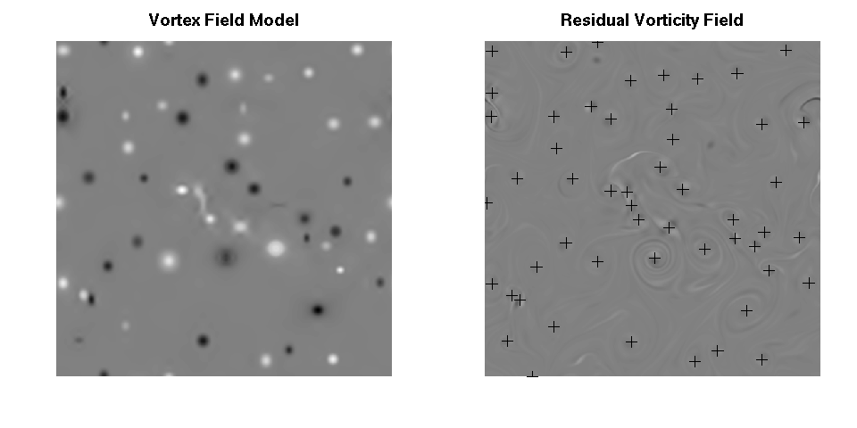
Figure 7: Candidate vortex locations, the vortex field model and residual field for the observed vorticity field at time $t=15$, plotted on the same grey scale. The spatial locations of the estimated coherent structures from the vortex field model are plotted on the residual field for comparison. Color changes in the locations of the candidate points are artificial and only meant to visualize points in areas of large negative vorticity.

A limitation of the current vortex field model is that elliptical structures, such as structures being warped by others in their local neighborhood, are not well modeled. Although the DWT decomposes two-dimensional structures into horizontal, vertical and diagonal features, warped vortices do not follow both diagonal directions simultaneously. Hence, the diagonal elements from the template function are not heavily utilized in the modeling process. Alternative wavelet transforms, such as the complex wavelet transform (Kingsbury kin:image,kin:complex), produce coefficients associated with several directions and have been more successful in representing structures in images when compared to common orthogonal wavelet filters. One could also apply other types of multi-scale transforms that are more efficient in representing and extracting other features of interest; e.g., the curvelet transform of sta-can-don:curvelet.

5.2 Application to Temporal Scaling

One scientific end point for studying a turbulence experiment is quantifying how coherent structures and their related statistics scale over time. Some examples of the analysis of two-dimensional turbulent flow are sie-wei:census using a wavelet-based procedure and the “objective observer” approach of mcw:vortices. We applied our new method to identify the vortices in all the vorticity fields at time $t\geq 7$. Figure 8 displays the number of vortices, average circulation, average enstrophy, and average maximum peak amplitude.

wei-mcw:temporal-scaling investigated the temporal scaling of vortex statistics using two techniques: long-time integration of the fluid equations and from a modified point-vortex model that describes turbulence as a set of interacting coherent structures. The two systems gave the same scaling exponent $\xi\approx{0.72}$. The scaling exponent measures the rate of decay of the turbulence and is governed by the dynamics of the vortex population. In addition, it provides a quantitative measure to test our algorithm. bra-etal:revisiting studied the evolution of vortex statistics from very high-resolution numerical simulations. The results of the numerical simulation at low Reynolds number found $\xi\approx{0.72}$, while the vortex decay rate at high Reynolds number was $\xi\approx{0.76}$. The Reynolds number is the ratio of inertial forces to viscous forces. Low Reynolds numbers correspond to Laminar flow where viscous forces dominate and is characterized by smooth, fluid motion and high Reynolds numbers are dominated by inertial forces and contain vortices and jets. The evolution of other vortex statistics can be expressed in terms of $\xi$ car-etal:evolution. The slopes with standard errors of the best fitting regression lines in Figure 8, from left to right and then top to bottom, are $-0.739$ (0.0127), 0.346 (0.0242), $-0.452$ (0.0232) and $-0.0337$ (0.0112) respectively. These values agree with those given in wei-mcw:temporal-scaling.

Figure 8: Temporal scaling of vortex statistics from the multiresolution-based census algorithm. All four quantities are expected to follow a scaling relation in time and are thus plotted on a log-log scale. The straight line in each plot is the best fitting regression line.

6 Discussion

Using a multiresolution multivariate regression model, we have been able to accurately model and extract coherent structures from a simulated two-dimensional fluid flow at high Reynolds number. The vortex statistics from analyzing each time step individually reproduces well-known empirical scaling behavior. This technique allows for an efficient, objective analysis of observed turbulent fields. Although these results have been achieved by previous algorithms, our method is not limited to simple accumulations of positive or negative vorticity. Through straightforward specification of the template function a variety of features may be extracted from turbulent flow. The modular implementation of our algorithm ensures flexibility across applications and precision of the results are guaranteed by using sound statistical techniques.

The methodology presented here can be directly transferred to a three-dimensional setting. For freely decaying, homogeneous geostrophic turbulence, coherent structures are compact regions of large vorticity organized in the vertical (so-called tubes); see, e.g., Farge et al. far-pel-sch:3D,far-pel-sch:zamm. Previous studies have only implemented a vortex census algorithm by adapting the “objective observer” approach of mcw:vortices. For the multiresolution approach, software implementations for the DWT and maximal overlap DWT are already available that extend computations to three dimensions. Further collaboration with experts in turbulence would be necessary, but a reasonable template function to try would be a three-dimensional Gaussian kernel or possibly a cylinder of fixed radius in $(x,y)$ and fixed height in the vertical direction.

sto-etal:asilomar recently proposed a novel statistical model for object tracking using an elliptical model for coherent structures. A distinct feature of this tracking model is that it allows splitting and merging of objects, and at the same time it also allows imperfect detection of objects at each time step (e.g., false positives). This tracking model has been, with preliminary success, applied to track the time evolution of coherent structures in turbulence. We see an opportunity to merge this technique with the methodology presented here in order to track the time evolution of the turbulent fluid using the regression coefficient matrix as a concise description of the coherent structure.

References

- [\citeauthoryearBracco, McWilliams, Murante, Provenzale, and WeissBracco et al.2000] Bracco, A., J. C. McWilliams, G. Murante, A. Provenzale, and J. B. Weiss (2000). Revisiting freely decaying two-dimensional turbulence at millennial resolution. Physics of Fluids 12(11), 2931–2941.
- [\citeauthoryearCarnevale, McWilliams, Pomeau, and YoungCarnevale et al.1991] Carnevale, G. F., J. C. McWilliams, Y. Pomeau, and W. R. Young (1991). Evolution of vortex statistics in two-dimensional turbulence. Physical Review Letters 66, 2735.
- [\citeauthoryearFarge, Goirand, Meyer, Pascal, and WickerhauserFarge et al.1992] Farge, M., E. Goirand, Y. Meyer, F. Pascal, and M. V. Wickerhauser (1992). Improved predictability of two-dimensional turbulent flows using wavelet packet compression. Fluid Dynamics Research 10, 229–250.
- [\citeauthoryearFarge, Kevlahan, Perrier, and GoirandFarge et al.1996] Farge, M., N. Kevlahan, V. Perrier, and E. Goirand (1996). Wavelets and turbulence. Proceedings of the IEEE 84(4), 639–669.
- [\citeauthoryearFarge, Pellegrino, and SchneiderFarge et al.2001a] Farge, M., G. Pellegrino, and K. Schneider (2001a). Coherent vortex extraction in 3D turbulent flows using orthogonal wavelets. Physical Review Letters 87(5), 054501.
- [\citeauthoryearFarge, Pellegrino, and SchneiderFarge et al.2001b] Farge, M., G. Pellegrino, and K. Schneider (2001b). Wavelet filtering of three-dimensional turbulence. Zeitschrift für Angewandte Mathematik und Mechanik 81(Suppl. 3), S465–S466.
- [\citeauthoryearFarge and PhilipovitchFarge and Philipovitch1993] Farge, M. and T. Philipovitch (1993). Coherent structure analysis and extraction using wavelets. In Y. Meyer and S. Roques (Eds.), Progress in Wavelet Analysis and Applications, pp. 477–481. Gif-sur-Yvette: Editions Frontièries.
- [\citeauthoryearFerzigerFerziger1996] Ferziger, J. H. (1996). Large eddy simulation. In T. B. Gatski, M. Y. Hussaini, and J. L. Lumley (Eds.), Simulation and Modelling of Turbulent Flows. Oxford University Press.
- [\citeauthoryearFriedman and StuetzleFriedman and Stuetzle1981] Friedman, J. H. and W. Stuetzle (1981). Projection pursuit regression. Journal of the American Statistical Association 76(376), 817–823.
- [\citeauthoryearFrischFrisch1995] Frisch, U. (1995). Turbulence. Cambridge: Cambridge University Press.
- [\citeauthoryearKingsburyKingsbury1999] Kingsbury, N. (1999). Image processing with complex wavelets. Philosophical Transactions of the Royal Society of London A 357, 2543–2560.
- [\citeauthoryearKingsburyKingsbury2001] Kingsbury, N. (2001). Complex wavelets for shift invariant analysis and filtering of signals. Applied and Computational Harmonic Analysis 10(3), 234–253.
- [\citeauthoryearKraichnan and MontgomeryKraichnan and Montgomery1980] Kraichnan, R. H. and D. Montgomery (1980). Two-dimensional turbulence. Reports on Progress in Physics 43(5), 547–619.
- [\citeauthoryearLesieurLesieur1997] Lesieur, M. (1997). Turbulence in Fluids. Dordrecht: Klewer Academic Publishers.
- [\citeauthoryearLuo and JamesonLuo and Jameson2001] Luo, J. and L. Jameson (2001). A wavelet-based technique for identifying, labeling, and tracking of ocean eddies. Journal of Atmospheric and Oceanic Technology 19(3), 381–390.
- [\citeauthoryearMallatMallat1998] Mallat, S. (1998). A Wavelet Tour of Signal Processing (1st ed.). San Diego: Academic Press.
- [\citeauthoryearMcWilliamsMcWilliams1984] McWilliams, J. (1984). The emergence of isolated coherent vortices in turbulent flow. Journal of Fluid Mechanics 146, 421–433.
- [\citeauthoryearMcWilliamsMcWilliams1990] McWilliams, J. C. (1990). The vortices of two-dimensional turbulence. Journal of Fluid Mechanics 219, 361–385.
- [\citeauthoryearMcWilliams and WeissMcWilliams and Weiss1994] McWilliams, J. C. and J. B. Weiss (1994). Anisotropic geophysical vortices. CHAOS 4, 305.
- [\citeauthoryearMoin and MaheshMoin and Mahesh1998] Moin, P. and K. Mahesh (1998). Direct Numerical Simulation: A tool in turbulence research. Annual Review of Fluid Mechanics 30(1), 539–578.
- [\citeauthoryearSiegel and WeissSiegel and Weiss1997] Siegel, A. and J. B. Weiss (1997). A wavelet-packet census algorithm for calculating vortex statistics. Physics of Fluids 9(7), 1988–1999.
- [\citeauthoryearStarck, Candes, and DonohoStarck et al.2002] Starck, J. L., E. J. Candes, and D. L. Donoho (2002). The curvelet transform for image denoising. IEEE Transactions on Image Processing 11(6), 670–684.
- [\citeauthoryearStorlie, Davis, Hoar, Lee, Nychka, Weiss, and WhitcherStorlie et al.2004] Storlie, C., C. Davis, T. Hoar, T. C. M. Lee, D. Nychka, J. Weiss, and B. Whitcher (2004). Identifying and tracking turbulence structures. In Proceedings of the 38th Asilomar Conference on Signals, Systems, and Computers, Pacific Grove, California, pp. 1700–1704.
- [\citeauthoryearVetterli and KovačevićVetterli and Kovačević1995] Vetterli, M. and J. Kovačević (1995). Wavelets and Subband Coding. New Jersey: Prentice Hall PTR.
- [\citeauthoryearWeiss and McWilliamsWeiss and McWilliams1993] Weiss, J. B. and J. C. McWilliams (1993). Temporal scaling behavior of decaying two-diemnsional turbulence. Physics of Fluids 5(3), 608–621.
- [\citeauthoryearWhitcher, Weiss, Nychka, and HoarWhitcher et al.2003] Whitcher, B., J. B. Weiss, D. W. Nychka, and T. J. Hoar (2003). Stochastic multiresolution models for turbulence. In M. G. Akritis and D. N. Politis (Eds.), Recent Advances and Trends in Nonparametric Statistics, pp. 497–509. Elsevier.
- [\citeauthoryearWickerhauser, Farge, and GoirandWickerhauser et al.1997] Wickerhauser, M. V., M. Farge, and E. Goirand (1997). Theoretical dimension and the complexity of simulated turbulence. In W. Dahmen, P. Oswald, and A. J. Kurdila (Eds.), Multiscale Wavlet Methods for Partial Differential Equations, Volume 6 of Wavelet Analysis and Applications, pp. 473–492. Boston: Academic Press.
- [\citeauthoryearWickerhauser, Farge, Goirand, Wesfreid, and CubilloWickerhauser et al.1994] Wickerhauser, M. V., M. Farge, E. Goirand, E. Wesfreid, and E. Cubillo (1994). Efficiency comparison of wavelet packet and adapted local cosine bases for compression of a two-dimensional turbulent flow. In C. K. Chui, L. Montefusco, and L. Puccio (Eds.), Wavelets: Theory, Algorithms, and Applications, pp. 509–531. San Diego, California: Academic Press.