Thiol density dependent classical potential for methyl-thiol on a Au(111) surface

Abstract

A new classical potential for methyl-thiol on a Au(111) surface has been developed using density functional theory electronic structure calculations. Energy surfaces between methyl-thiol and a gold surface were investigated in terms of symmetry sites and thiol density. Geometrical optimization was employed over all the configurations while minimum energy and thiol height were determined. Finally, a new interatomic potential has been generated as a function of thiol density, and applications to coarse-grained simulations are presented.

I Introduction

Understanding the structural features of well-ordered self-assembled monolayers Dubois and Nuzzo (1992); Ulman (1996); Schreiber (2000); Zhang et al. (2003) requires a detailed potential energy surface of alkanethiols adsorbed onto metallic surfaces. Thiol headgroups bridge alkane chains with metal surfaces such as gold, and play key roles in deciding the properties of surface self-assembly. Extensive theoretical studies thereby have been done to explore the thiol interaction with a gold surface through electronic structure models Beardmore et al. (1998); Grönbeck et al. (2000); Hayashi et al. (2001); Yourdshahyan et al. (2001); Yourdshahyan and Rappe (2002); Morikawa et al. (2002); Gottschalck and Hammer (2002); Renzi et al. (2004); Masens et al. (2005); Cometto et al. (2005). These investigations have revealed that the overall binding energy is found as around 40kcal/mol, and the binding energy varies with the relative sulfur position on the gold lattice. Also, additional experimental and computational results indicate that neighboring thiol configuration may affect the thiol-gold binding Schreiber (2000). However, the lateral energy-corrugation of the surface by the underlying atomic gold lattice has not yet been completely understood.

The purpose of this thiol-gold interaction investigation is two-fold. First, the self-assembled monolayer of alkanethiol on gold has become a de facto standard for understanding surface self-assembly of micro and nanostructures. Profiling the atomic scale energy surface is fundamental to comprehending the experimental observations of domain formation and structural defects. Secondly, explicit description of the energy surface can be formulated as classical potentials, which allow large scale molecular dynamics (MD) Grønbech-Jensen et al. (2003) or Monte Carlo (MC) simulations.

We have conducted extensive electronic structure calculations of thiol-gold interactions in order to build a new classical potential, which incorporates the sulfur position relative to the gold lattice and the many-body effects from adjacent thiols. This study is an extension of the previous work of classical potentials for MD and MC simulations Beardmore et al. (1998). The previous potential was developed using a dilute thiol model (one thiol on an isolated gold cluster). The results indicated that a fully optimized thiol on gold prefers the hollow sites, and the FCC site is more stable than HCP. The results have subsequently been verified hic , but later experiments and numerical calculations Yourdshahyan et al. (2001); Yourdshahyan and Rappe (2002); Renzi et al. (2004) have also revealed that Bridge or hybrid sites may provide the global minimum. Our present results, which are based on non-zero thiol density, substantiate these later findings.

The rest of the paper is organized as follows. First we briefly describe our ab initio calculations and summarize the results. Then the classical potential, which has been fitted to the results of the electronic structure optimizations, will be presented. Before concluding the paper, several applications of the new potential within MD simulations are exemplified with specific thiol densities on a Au(111) surface.

II ab initio calculations

Advances in computational capacity and algorithmic efficiency of first-principle calculations have greatly improved the quality and consistency of numerical simulations of, e.g., thiol on gold. In the previous study Beardmore et al. (1998), quantum chemistry techniques with a small finite size of gold cluster model was employed to produce an energy surface as a function of thiol position and orientation. However, periodic boundary conditions (PBC), which imitates a non-zero thiol density, can simulate more realistic configurations and is found to efficiently produce reliable results Grönbeck et al. (2000); Hayashi et al. (2001); Yourdshahyan and Rappe (2002); Cometto et al. (2005). We have therefore employed the band structure simulation code VASP Kresse and Furthmüller (1996a, b) to conduct density functional theory (DFT) Hohenberg and Kohn (1964); Kohn and Sham (1965) simulations of various energy surfaces. The Projector Augmented Wave (PAW) Blöchl (1994); Kresse and Joubert (1999) potential was used for electron-ion interactions and the Generalized Gradient Approximation (GGA) Perdew and Wang (1992) was applied for exchange correlation with a plane wave basis. For plane waves, a 400eV cutoff energy was implemented. Even though plane periodic images are included in the calculation to simulate dense thiol states, the effect from surface normal periodicity was excluded by inserting 10Å vacuum layer above the unit-cell. We used $4\times 4\times 1$ k-points for the Monkhorst-Pack grid. With those configurations, ab initio simulations were done for various thiol densities and positions.

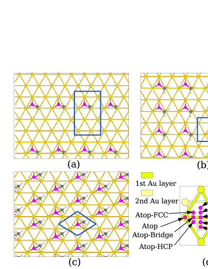
Figure 1: (Color online) Unit-cells with periodic boundary condition: (a) $2\!\times\!4$ cell, (b) $2\!\times\!2$ cell, (c) $\sqrt{3}\!\times\!\sqrt{3}\rm R30^{o}$, (d) nine sampling points for landscape variations on a Au(111) surface.

With periodic boundary conditions, several surface unit-cells were investigated in order to mimic thiol density effects. The specific periodicities are: $2\!\times\!4$, $2\!\times\!2$, and $\sqrt{3}\!\times\!\sqrt{3}\rm R30^{o}$ of Au(111) unit-cells with a single methyl-thiol. The lattices are depicted in Figure 1. Figure 1-(a) shows the $2\!\times\!4$ unit-cell with 8 gold atoms per single gold layer. Figure 1-(b) shows the $2\!\times\!2$ unit-cell with gold layers of 4 atoms. The $\sqrt{3}\!\times\!\sqrt{3}\rm R30^{o}$ unit-cell, shown in Figure 1-(c), represents the maximum thiol packing density (full coverage) of a Au(111) surface Ulman (1996) (Note that the precise location of the unit-cells are not accurately represented in Figure 1).

In order to evaluate the energy surface on symmetric sites, nine sampling points were selected, including Atop, Bridge, FCC, HCP, and hybrid points in between. These points are illustrated in Figure 1-(d).

The methyl-thiol binding energy to the Au(111) surface is determined by comparing the energies of relaxed models of Au(111) with and without the methyl-thiol:

$$E_{\rm bind}=E_{\rm Au(111)+SCH_{3}}-E_{\rm Au(111)}-E_{\rm SCH_{3}}$$ (1)

II.1 Effect of Au(111) thickness

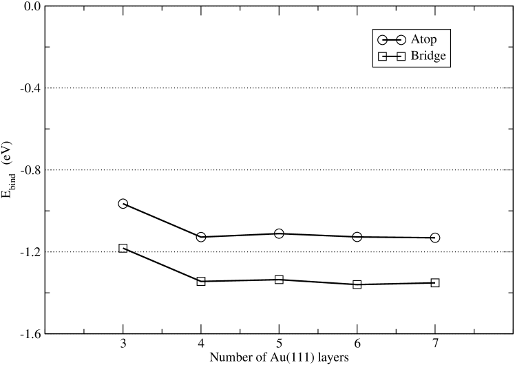
Figure 2: The effect of gold layer thickness on the binding energy of methyl-thiol on a Au(111) surface. For more than four layers, binding energies are saturated.

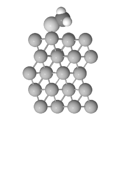
Figure 3: Side view of methyl-thiol on Au(111) of a five-layer slab.

It is known that a small number of atomic layers of gold will influence the calculated binding energy Yourdshahyan et al. (2001). We therefore determine an acceptable number of gold layers as follows: Atop and Bridge sites are found as global maximum and minimum Yourdshahyan et al. (2001); Yourdshahyan and Rappe (2002), and can therefore serve as standard points for a gold layer effect study. Atop and Bridge sites on a $\sqrt{3}\!\times\!\sqrt{3}\rm R30^{o}$ unit-cell were configured with various numbers of Au(111) layers (with lattice constant=4.08 Å), and tested by the ab initio calculations described above. The bottom layer was fixed and upper layers were relaxed along the normal direction. Simulation results are provided in Figure 2 where the effect of the number of gold layers is illustrated. More than four layers, binding energies for both points saturate. Also, the energy difference between the two points is maintained when more than four gold lattice layers are simulated. We conclude that at least four layers are required to adequately calculate the binding energy. We employed five Au(111) layers for the binding energy calculations of above mentioned nine sampling points, as illustrated in Figure 3.

II.2 ab initio calculation results

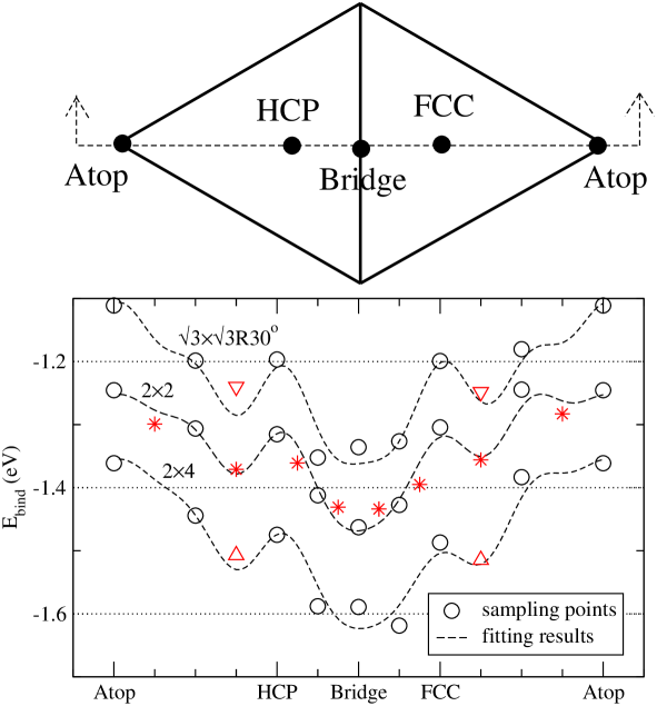
Figure 4: (Color online) ab-initio results of sampling points and the fitting results. Down triangles are the results of fine analysis of $\sqrt{3}\!\times\!\sqrt{3}\rm R30^{o}$ unit-cell, while asterisks(*) for $2\!\times\!2$ and up triangles for $2\!\times\!4$ unit-cell. These test points are not included in the fitting.

All nine points [Figure 1-(d)] on the Au(111) surface were probed with different thiol densities, and the results are summarized in Table 1. Also selected results are provided in Figure 4 along the Atop-Bridge-Atop path. Even though thiol density affects the magnitude of binding energies, lateral corrugations of the energy were found to be similar for all three densities. The Atop site was the least stable and the FCC sites were slightly more stable than HCP although the difference is negligible. Finally, Bridge and hybrid sites of Bridge-FCC and Bridge-HCP present the strongest binding energy, in agreement with other recent studies Hayashi et al. (2001); Yourdshahyan and Rappe (2002); Gottschalck and Hammer (2002); Cometto et al. (2005). Overall binding energy increases as thiol density decreases, while lateral corrugation seems largely unaffected. Even though global minimum points move from HCP-Bridge site to FCC-Bridge site, but the difference is not distinct. In other words, global minimum and maximum sites are not significantly changed by the variations of thiol density, whereas local thiol density determines the magnitude of the binding energy. Thus, thiol-position and local thiol-density can be decoupled in a classical potential function such that a many-body component to the energy surface provides mutual thiol repulsion.

In addition to the binding energies, optimized vertical distances between thiol and Au(111) surface were investigated. Similarly to the binding energy results, an Atop positioning of thiol showed the largest distance, while optimized thiol distances to FCC and HCP sites are small. An interesting point is that these results are quite similar regardless of thiol density. Consequently, our fitting of the thiol-Au(111) distance surface was done without a thiol density term.

III Generation of energy surfaces of classical potentials

Based on the previous work Beardmore et al. (1998), we have interpolated and fitted the electronic structure results with harmonic functions to compose an egg-box type surface, which can reproduce three-fold symmetry. With following characteristic vectors and harmonic sums, all the 3-fold symmetric sites of the Au(111) surface are periodically represented:

$${\bf k}_{1}=k_{0}\left({\sqrt{3}\over 2},{1\over 2}\right),~{}~{}{\bf k}_{2}=k_{0}\left(-{\sqrt{3}\over 2},{1\over 2}\right),~{}~{}{\bf k}_{3}=k_{0}\left(0,-1\right),$$ (2)

where $k_{0}=4\pi/{\sqrt{3}}a$, and $a$ is the inter-atomic distance for gold (=2.884Å). Using basic and high order harmonic functions, energy surfaces were determined. The fitting functions for the binding energies are shown below.

$$E_{\rm bind} = a_{0}+a_{1}\sum_{i=1}^{3}\cos({\bf k}_{i}\cdot{\bf x})+a_{2}\sum_{i=1}^{3}\sin({\bf k}_{i}\cdot{\bf x})+a_{3}\sum_{i=1}^{3}\cos(2{\bf k}_{i}\cdot{\bf x})$$ (3)

$$+a_{4}\sum_{i=1}^{3}\sin(2{\bf k}_{i}\cdot{\bf x})+a_{5}\sum_{i=1}^{3}\cos(3{\bf k}_{i}\cdot{\bf x}).$$

For high-order harmonics, we included up to third harmonics but the sin function of third order was excluded due to negligible contributions. All fitting coefficients are summarized in Table 2 for each thiol density. They are interpolated using a cubic spline, and surface coefficients for an intermediate density are given as

$$a_{i}=s_{3}\cdot\bar{\rho}^{3}+s_{2}\cdot\bar{\rho}^{2}+s_{1}\cdot\bar{\rho}+s_{0}.$$ (4)

Cubic spline coefficients $s_{i}$ are provided in Table 3, where the thiol density is normalized to that of the $2\!\times\!2$ unit-cell.

With the above equations, the binding energy is addressed in terms of thiol density and position. The comparison to the sampling points are illustrated in Figure 4. Rms error of 27 sampling points was calculated as 0.018 eV. The fitted energy surface is seen to represent the sampling point data quite well with the selected level of harmonic functions. However, the fitted function has variations that are not directly given by the sample points. In order to investigate if this variation is an artifact of the fitting function, we have chosen to compare the fitting result to twelve additional energies derived at intermediate thiol surface locations: eight additional for one of the thiol densities (2x2 unit-cell) and two additional for each of the other two densities. These are represented with asterisks (*) and triangles. It is evident from the comparison in Figure 4 that the fitted energy curve represents also the independent validation points very well, and so, we submit that the presented fitting is representative of the surface generated from ab initio methods.

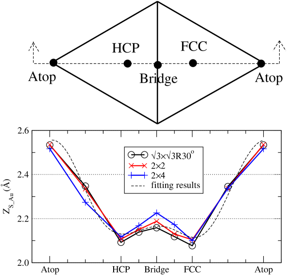
Figure 5: (Color online) The thiol-Au(111) distance along symmetric sites. The effect of thiol density change is not distinct in the thiol-Au(111) distance, and a single fitting surface is employed.

The fitting method was also used for the optimized thiol-Au(111) distance surface. The fitting functions are shown below and a comparison to the ab initio data is plotted in Figure 5.

$$Z_{\rm S\_Au} = b_{0}+b_{1}\sum_{i=1}^{3}\cos({\bf k}_{i}\cdot{\bf x})+b_{2}\sum_{i=1}^{3}\sin({\bf k}_{i}\cdot{\bf x})$$ (5)

$$+b_{3}\sum_{i=1}^{3}\cos(2{\bf k}_{i}\cdot{\bf x})+b_{4}\sum_{i=1}^{3}\sin(2{\bf k}_{i}\cdot{\bf x})$$

Unlike the binding energy, this fitting is not affected by thiol density and it is therefore shown in terms of thiol position only. Fitting coefficients of the distance surface are summarized in Table 4. From the fitting results, a sample energy surface of a $2\!\times\!4$ unit-cell and the corresponding thiol-Au(111) distance surface is illustrated in Figure 6. Atop sites are located (in Å) at (0,0), (2.884,0), and (1.442,2.498) while HCP is at (1.442,0.833). All other symmetric sites can be mapped along three fold symmetry. Atop sites are seen to be energetic maxima whereas thiols near Bridge sites show the strongest binding to the surface. Other thiol densities have similar energy surfaces. On the distance surface, peaks are found around Atop, but the Bridge site is slightly higher than the hollow sites. FCC and HCP show similar heights. We notice, however, that the variation in height observed in Figure 6, is less than 1Å, indicating that the height variation is not an important component for describing surface self-assemblies.

In essence, the fitting coefficients of energy surfaces are determined by a local thiol density, and we have to collect the effects of neighboring thiols. The embedded atom method (EAM) Daw and Baskes (1984) employs the local density to incorporate many-body effects into classical MD potentials. For that purpose, we determine the local thiol density $\rho_{i}$ as

$$\rho_{i}=\sum_{j}\rho(r_{ij}),$$ (6)

where $r_{ij}$ is the distance between the given thiol i and all adjacent thiols j. Each neighbor contributes to the density $\rho_{i}$ of the ith thiol through the function $\rho$. Using the following function, the local thiol density can be defined as

$$\rho(r_{ij}) = \left\{\begin{array}[]{clr}\big{\{}1-\cos\left({2\pi(r_{ij}-5a)\over 5a}\right)\big{\}}/2{}{}{}&{\rm if}&r_{ij}<5a\\ 0&{\rm if}&r_{ij}\geq 5a\end{array}\right.,$$ (9)

where $a$ is the inter-atomic distance for gold (=2.884Å). The formulation of local density reproduces the corresponding densities with our chosen unit-cells: $2\!\times\!4$, $2\!\times\!2$, and $\sqrt{3}\!\times\!\sqrt{3}\rm R30^{o}$. We therefore adopt the form (9) to include a thiol density into the calculation of the binding energy ($E_{\rm bind}$).

We finally combine the local thiol density and position into a Morse potential:

$$V(\rho_{i},{\bf x}_{i},z_{i}) = E_{\rm bind}(\rho_{i},{\bf x}_{i})\cdot\Big{\{}\exp[-2\beta_{e}(z_{i}-Z_{\rm S\_Au}({\bf x}_{i}))]\Big{.}$$ (10)

$$-2\exp[-\beta_{e}(z_{i}-Z_{\rm S\_Au}({\bf x}_{i}))]\Big{.}\Big{\}}.$$

Here, $z_{i}$ is the normal distance between the thiol and the Au(111) surface at the position ${\bf x}_{i}$, and $\beta_{e}$ is the curvature of the potential. To determine the potential curvature, perturbations to the thiol-Au distances were given on the optimized states. Energy differences and the gradient were calculated along the distance variations. It was found empirically that the gradient is proportional to $Z_{\rm S\_Au}$ as

$$\beta_{e}=c_{1}Z_{\rm S\_Au}.$$ (11)

The constant $c_{1}$ is a function of the local thiol density and calculated with a cubic spline similarly to Eq.(4). All parameters are summarized in Table. 5.

IV Application to classical molecular dynamics simulations

In order to demonstrate the practical applications of the developed potential, we have simulated methyl-thiol headgroup distributions on Au(111) for several surface coverages. Classical MD has been implemented with a united atom force field Hautman and Klein (1989) for the chain-chain interactions, and RATTLE Andersen (1983) for constraints of the carbon-carbon bond lengths and angles. The torsional potential for dihedral angles were adopted from Hautman and Klein (1989), and the thiol headgroup potential was incorporated using Eq.(3).

Decanethiols are distributed along the simulation cell of 86.52Å$\times$ 79.92 Å and periodic boundary conditions are imposed. Coverages are 1/2, 2/3, and 1 of optimal coverage with 160, 210, and 320 decanethiols, respectively. A stochastic thermostat Hünenberger (2005) was set at 300K and the system was relaxed for 100ps.

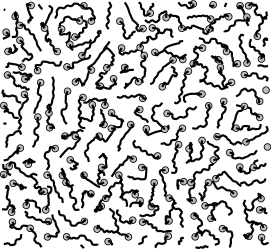
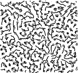
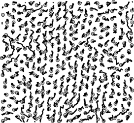
Figure 7: Top view of alkane chains (black line) and thiol headgroups (grey circle) on gold surface from MD simulations (left: 1/2 coverage, middle: 2/3 coverage, right: full coverage).

Figure 7 shows top views of the MD results using the developed headgroup potentials. At low density the alkane chains lie between neighboring chains and the headgroups show irregular patterns. As coverage increases, alkane chains interact with each other and lift from the surface. At high density the headgroups order hexagonally, and alkane chains tilt toward NN (Nearest Neighbor) or NNN (Next Nearest Neighbor). In order to investigate headgroup distributions along the characteristic line (Atop-HCP-Bridge-FCC-Atop), their locations at each coverage were examined and normalized histograms are presented in Figure 8. For all coverages, most of the headgroups are found between HCP-Bridge and FCC-Bridge hybrid sites. This result is consistent with the energetics of the electronic structure calculations.

V Conclusion and discussion

In summary, electronic structure calculations have been conducted to characterize the details of interactions between methyl-thiol and Au(111) surfaces. The energy surface has been studied as a function of thiol location and density. The results are consistent with other recent work, and a new classical potential has been developed from the results. The potential is completely parametrized, and its application to MD is demonstrated. Large scale molecular dynamics simulations are under way to explore the domain formation and structure composition of surface self-assembly using the surface potential developed in this paper.

V.1 Acknowledgments

This work was carried out under the auspices of the National Nuclear Security Administration of the U.S. Department of Energy at Los Alamos National Laboratory under Contract No. DE-AC52-06NA25396 and the Cooperative Agreement on Research and Education (CARE) for UCDRD funding. Partial support was provided by the National Science Foundation Biophotonics Science and Technology Center (University of California at Davis).

Table 1: ab initio results of binding energy ($E_{\rm bind}$) in terms of symmetric sites for each unit-cell.

unit-cell	$~{}~{}~{}~{}2\!\times\!4~{}~{}~{}~{}$	$~{}~{}~{}~{}2\!\times\!2~{}~{}~{}~{}$	$\sqrt{3}\!\times\!\sqrt{3}\rm R30^{o}$
ATOP	-1.361	-1.245	-1.111
Bridge	-1.589	-1.463	-1.336
FCC	-1.487	-1.304	-1.199
HCP	-1.475	-1.315	-1.197
Atop-Bridge	-1.402	-1.290	-1.158
Atop-HCP	-1.444	-1.306	-1.199
Atop-FCC	-1.383	-1.245	-1.181
FCC-Bridge	-1.619	-1.427	-1.326
HCP-Bridge	-1.586	-1.412	-1.352

Table 2: Egg-box fitting parameters of binding energy ($E_{\rm bind}$) for each unit-cell.

unit-cell	$2\!\times\!4~{}~{}~{}~{}~{}$	$2\!\times\!2~{}~{}~{}~{}~{}~{}$	$\sqrt{3}\!\times\!\sqrt{3}\rm R30^{o}$
$a_{0}$	$-1.481\times 10^{-0}$	$-1.335\times 10^{-0}$	$-1.233\times 10^{-0}$
$a_{1}$	$5.451\times 10^{-2}$	$4.009\times 10^{-2}$	$4.285\times 10^{-2}$
$a_{2}$	$3.218\times 10^{-3}$	$6.910\times 10^{-3}$	$4.236\times 10^{-3}$
$a_{3}$	$-2.497\times 10^{-2}$	$-2.607\times 10^{-2}$	$-2.134\times 10^{-2}$
$a_{4}$	$9.041\times 10^{-3}$	$8.068\times 10^{-3}$	$2.897\times 10^{-3}$
$a_{5}$	$1.266\times 10^{-2}$	$1.375\times 10^{-2}$	$2.093\times 10^{-2}$

Table 3: Cubic spline coefficients for egg-box fitting parameters of binding energy (in eV). $\bar{\rho}$ = normalized thiol density.

	$0.5<\bar{\rho}<1.0$
	$s_{3}~{}~{}~{}~{}~{}~{}~{}~{}~{}$	$s_{2}~{}~{}~{}~{}~{}~{}~{}~{}~{}$	$s_{1}~{}~{}~{}~{}~{}~{}~{}~{}~{}$	$s_{0}~{}~{}~{}~{}~{}~{}~{}~{}~{}$
$a_{0}$	$1.760\times 10^{-2}$	$-2.641\times 10^{-2}$	$3.005\times 10^{-1}$	$-1.627\times 10^{-0}$
$a_{1}$	$4.458\times 10^{-2}$	$-6.686\times 10^{-2}$	$-6.546\times 10^{-3}$	$6.892\times 10^{-2}$
$a_{2}$	$-1.851\times 10^{-2}$	$2.776\times 10^{-2}$	$-1.871\times 10^{-3}$	$-4.737\times 10^{-4}$
$a_{3}$	$1.968\times 10^{-2}$	$-2.952\times 10^{-2}$	$7.647\times 10^{-3}$	$-2.387\times 10^{-2}$
$a_{4}$	$-1.631\times 10^{-2}$	$2.447\times 10^{-2}$	$-1.010\times 10^{-2}$	$1.001\times 10^{-2}$
$a_{5}$	$2.326\times 10^{-2}$	$-3.488\times 10^{-2}$	$1.382\times 10^{-2}$	$1.156\times 10^{-2}$
	$1.0<\bar{\rho}<1.33$
	$s_{3}~{}~{}~{}~{}~{}~{}~{}~{}~{}$	$s_{2}~{}~{}~{}~{}~{}~{}~{}~{}~{}$	$s_{1}~{}~{}~{}~{}~{}~{}~{}~{}~{}$	$s_{0}~{}~{}~{}~{}~{}~{}~{}~{}~{}$
$a_{0}$	$-2.644\times 10^{-2}$	$1.057\times 10^{-1}$	$1.684\times 10^{-1}$	$-1.583\times 10^{-0}$
$a_{1}$	$-6.696\times 10^{-2}$	$2.677\times 10^{-1}$	$-3.411\times 10^{-1}$	$1.805\times 10^{-1}$
$a_{2}$	$2.780\times 10^{-2}$	$-1.112\times 10^{-1}$	$1.371\times 10^{-1}$	$-4.678\times 10^{-2}$
$a_{3}$	$-2.956\times 10^{-2}$	$1.182\times 10^{-1}$	$-1.401\times 10^{-1}$	$2.537\times 10^{-2}$
$a_{4}$	$2.450\times 10^{-2}$	$-9.798\times 10^{-2}$	$1.123\times 10^{-1}$	$-3.080\times 10^{-2}$
$a_{5}$	$-3.493\times 10^{-2}$	$1.397\times 10^{-1}$	$-1.607\times 10^{-1}$	$6.975\times 10^{-2}$

Table 4: Egg-box fitting parameters of the thiol-Au distance surface ($Z_{\rm S\_Au}$) for each unit-cell (unit:Å).

$b_{0}$	$b_{1}~{}~{}~{}~{}~{}~{}$	$b_{2}~{}~{}~{}~{}~{}~{}$	$b_{3}~{}~{}~{}~{}~{}~{}$	$b_{4}~{}~{}~{}~{}~{}~{}$
$2.267\times 10^{-0}$	$9.771\times 10^{-2}$	$5.552\times 10^{-4}$	$-1.262\times 10^{-3}$	$3.516\times 10^{-3}$

Table 5: Cubic spline coefficients for the curvature of thiol potential. $\bar{\rho}$ = normalized thiol density.

	$0.5<\bar{\rho}<1.0$
	$s_{3}~{}~{}~{}~{}~{}$	$s_{2}~{}~{}~{}~{}~{}$	$s_{1}~{}~{}~{}~{}~{}$	$s_{0}~{}~{}~{}~{}~{}$
$c_{1}$	$-9.660\times 10^{-3}$	$1.449\times 10^{-2}$	$3.545\times 10^{-2}$	$4.536\times 10^{-2}$
	$1.0<\bar{\rho}<1.33$
	$s_{3}~{}~{}~{}~{}~{}$	$s_{2}~{}~{}~{}~{}~{}$	$s_{1}~{}~{}~{}~{}~{}$	$s_{0}~{}~{}~{}~{}~{}$
$c_{1}$	$1.451\times 10^{-2}$	$-5.802\times 10^{-2}$	$1.080\times 10^{-1}$	$2.119\times 10^{-2}$

Figure 6: (Upper) Energy surface for $2\!\times\!4$ cell. For the other thiol density models, the shapes of energy surfaces are consistent with some changes of magnitude. (Lower) Thiol-Au(111) distance surface.

Figure 8: Distribution of headgroups along symmetric sites from MD simulations. They are normalized distributions and consistently headgroups are found around Bridge site with high probabilities.

References

- Dubois and Nuzzo (1992) L. H. Dubois and R. G. Nuzzo, Annual Reviews in Physical Chemistry 43, 437 (1992).
- Ulman (1996) A. Ulman, Chemical Reviews 96, 1533 (1996).
- Schreiber (2000) F. Schreiber, Progress in Surface Science 65, 151 (2000).
- Zhang et al. (2003) J. Z. Zhang, Z. Wang, J. Liu, S. Chen, and G. Liu, Self-Assembled Nanostructures (Kluwer Academic/Plenum, 2003).
- Beardmore et al. (1998) K. M. Beardmore, J. D. Kress, N. Grønbech-Jensen, and A. Bishop, Chemical Physics Letters 286, 40 (1998).
- Grönbeck et al. (2000) H. Grönbeck, A. Curioni, and W. Adreoni, Journal of American Chemical Society 122, 3839 (2000).
- Hayashi et al. (2001) T. Hayashi, Y. Morikawa, and H. Nozoye, Journal of Chemical Physics 114, 7615 (2001).
- Yourdshahyan et al. (2001) Y. Yourdshahyan, H. K. Zhang, and A. M. Rappe, Physical Review B 63, 081405(R) (2001).
- Yourdshahyan and Rappe (2002) Y. Yourdshahyan and A. M. Rappe, Journal of Chemical Physics 117, 825 (2002).
- Morikawa et al. (2002) Y. Morikawa, T. Hayashi, C. Liew, and H. Nozoye, Surface Science 507-510, 46 (2002).
- Gottschalck and Hammer (2002) J. Gottschalck and B. Hammer, Journal of Chemical Physics 116, 784 (2002).
- Renzi et al. (2004) V. D. Renzi, R. D. Felice, D. Marchetto, R. Biagi, U. del Pennino, and A. Selloni, Journal of Physical Chemistry B 108, 16 (2004).
- Masens et al. (2005) C. Masens, M. J. Ford, and M. B. Cortie, Surface science 580, 19 (2005).
- Cometto et al. (2005) F. P. Cometto, P. Paredes-Olivera, V. A. Macagno, and E. M. Patrito, Journal of physical chemistry B 109, 21737 (2005).
- Grønbech-Jensen et al. (2003) N. Grønbech-Jensen, A. N. Parikh, K. M. Beardmore, and R. C. Desai, Langmuir 19, 1474 (2003).
- (16) The favored gold(111) fcc hollow site positioning of single thiols has been reconfirmed by more recent extensive DFT calculations in, for example, refYourdshahyan et al. (2001); Yourdshahyan and Rappe (2002). Unfortunately, those publications have erroneously quoted ref Beardmore et al. (1998) as suggesting the hcp hollow site is the energetically preferred location of thiols.
- Kresse and Furthmüller (1996a) G. Kresse and J. Furthmüller, Computational materials science 6, 15 (1996a).
- Kresse and Furthmüller (1996b) G. Kresse and J. Furthmüller, Physical Review B 54, 11169 (1996b).
- Hohenberg and Kohn (1964) P. Hohenberg and W. Kohn, Physical Review 136, 864 (1964).
- Kohn and Sham (1965) W. Kohn and L. J. Sham, Physical Review 140, 1133 (1965).
- Blöchl (1994) P. E. Blöchl, Physical Review B 50, 17953 (1994).
- Kresse and Joubert (1999) G. Kresse and D. Joubert, Physical Review B 59, 1758 (1999).
- Perdew and Wang (1992) J. P. Perdew and Y. Wang, Physical Review B 45, 13244 (1992).
- Daw and Baskes (1984) M. S. Daw and M. I. Baskes, Physical Review B 29, 6443 (1984).
- Hautman and Klein (1989) J. Hautman and M. L. Klein, Journal of Chemical Physics 91, 4994 (1989).
- Andersen (1983) H. C. Andersen, Journal of Computational Physics 52, 24 (1983).
- Hünenberger (2005) P. H. Hünenberger, Advances in Polymer Science 173, 105 (2005).