The nested Chinese restaurant process and Bayesian nonparametric inference of topic hierarchies

Abstract.

We present the nested Chinese restaurant process (nCRP), a stochastic process which assigns probability distributions to infinitely-deep, infinitely-branching trees. We show how this stochastic process can be used as a prior distribution in a Bayesian nonparametric model of document collections. Specifically, we present an application to information retrieval in which documents are modeled as paths down a random tree, and the preferential attachment dynamics of the nCRP leads to clustering of documents according to sharing of topics at multiple levels of abstraction. Given a corpus of documents, a posterior inference algorithm finds an approximation to a posterior distribution over trees, topics and allocations of words to levels of the tree. We demonstrate this algorithm on collections of scientific abstracts from several journals. This model exemplifies a recent trend in statistical machine learning—the use of Bayesian nonparametric methods to infer distributions on flexible data structures.

1. Introduction

For much of its history, computer science has focused on deductive formal methods, allying itself with deductive traditions in areas of mathematics such as set theory, logic, algebra, and combinatorics. There has been accordingly less focus on efforts to develop inductive, empirically-based formalisms in computer science, a gap which became increasingly visible over the years as computers have been required to interact with noisy, difficult-to-characterize sources of data, such as those deriving from physical signals or from human activity. In more recent history, the field of machine learning has aimed to fill this gap, allying itself with inductive traditions in probability and statistics, while focusing on methods that are amenable to analysis as computational procedures.

Machine learning methods can be divided into supervised learning methods and unsupervised learning methods. Supervised learning has been a major focus of machine learning research. In supervised learning, each data point is associated with a label (e.g., a category, a rank or a real number) and the goal is to find a function that maps data into labels (so as to predict the labels of data that have not yet been labeled). A canonical example of supervised machine learning is the email spam filter, which is trained on known spam messages and then used to mark incoming unlabeled email as spam or non-spam.

While supervised learning remains an active and vibrant area of research, more recently the focus in machine learning has turned to unsupervised learning methods. In unsupervised learning the data are not labeled, and the broad goal is to find patterns and structure within the data set. Different formulations of unsupervised learning are based on different notions of “pattern” and “structure.” Canonical examples include clustering, the problem of grouping data into meaningful groups of similar points, and dimension reduction, the problem of finding a compact representation that retains useful information in the data set. One way to render these notions concrete is to tie them to a supervised learning problem; thus, a structure is validated if it aids the performance of an associated supervised learning system. Often, however, the goal is more exploratory. Inferred structures and patterns might be used, for example, to visualize or organize the data according to subjective criteria. With the increased access to all kinds of unlabeled data—scientific data, personal data, consumer data, economic data, government data, text data—exploratory unsupervised machine learning methods have become increasingly prominent.

Another important dichotomy in machine learning distinguishes between parametric and nonparametric models. A parametric model involves a fixed representation that does not grow structurally as more data are observed. Examples include linear regression and clustering methods in which the number of clusters is fixed a priori. A nonparametric model, on the other hand, is based on representations that are allowed to grow structurally as more data are observed. Nonparametric approaches are often adopted when the goal is to impose as few assumptions as possible and to “let the data speak.”

The nonparametric approach underlies many of the most significant developments in the supervised learning branch of machine learning over the past two decades. In particular, modern classifiers such as decision trees, boosting and nearest neighbor methods are nonparametric, as are the class of supervised learning systems built on “kernel methods,” including the support vector machine. (See Hastie et al. (2001) for a good review of these methods.) Theoretical developments in supervised learning have shown that as the number of data points grows, these methods can converge to the true labeling function underlying the data, even when the data lie in an uncountably infinite space and the labeling function is arbitrary (Devroye et al., 1996). This would clearly not be possible for parametric classifiers.

The assumption that labels are available in supervised learning is a strong assumption, but it has the virtue that few additional assumptions are generally needed to obtain a useful supervised learning methodology. In unsupervised learning, on the other hand, the absence of labels and the need to obtain operational definitions of “pattern” and “structure” generally makes it necessary to impose additional assumptions on the data source. In particular, unsupervised learning methods are often based on “generative models,” which are probabilistic models that express hypotheses about the way in which the data may have been generated. Probabilistic graphical models (also known as “Bayesian networks” and “Markov random fields”) have emerged as a broadly useful approach to specifying generative models (Lauritzen, 1996; Jordan, 2000). The elegant marriage of graph theory and probability theory in graphical models makes it possible to take a fully probabilistic (i.e., Bayesian) approach to unsupervised learning in which efficient algorithms are available to update a prior generative model into a posterior generative model once data have been observed.

Although graphical models have catalyzed much research in unsupervised learning and have had many practical successes, it is important to note that most of the graphical model literature has been focused on parametric models. In particular, the graphs and the local potential functions comprising a graphical model are viewed as fixed objects; they do not grow structurally as more data are observed. Thus, while nonparametric methods have dominated the literature in supervised learning, parametric methods have dominated in unsupervised learning. This may seem surprising given that the open-ended nature of the unsupervised learning problem seems particularly commensurate with the nonparametric philosophy. But it reflects an underlying tension in unsupervised learning—to obtain a well-posed learning problem it is necessary to impose assumptions, but the assumptions should not be too strong or they will inform the discovered structure more than the data themselves.

It is our view that the framework of Bayesian nonparametric statistics provides a general way to lessen this tension and to pave the way to unsupervised learning methods that combine the virtues of the probabilistic approach embodied in graphical models with the nonparametric spirit of supervised learning. In Bayesian nonparametric (BNP) inference, the prior and posterior distributions are no longer restricted to be parametric distributions, but are general stochastic processes Hjort et al. (2009). Recall that a stochastic process is simply an indexed collection of random variables, where the index set is allowed to be infinite. Thus, using stochastic processes, the objects of Bayesian inference are no longer restricted to finite-dimensional spaces, but are allowed to range over general infinite-dimensional spaces. For example, objects such as trees of arbitrary branching factor and arbitrary depth are allowed within the BNP framework, as are other structured objects of open-ended cardinality such as partitions and lists. It is also possible to work with stochastic processes that place distributions on functions and distributions on distributions. The latter fact exhibits the potential for recursive constructions that is available within the BNP framework. In general, we view the representational flexibility of the BNP framework as a statistical counterpart of the flexible data structures that are ubiquitous in computer science.

In this paper, we aim to introduce the BNP framework to a wider computational audience by showing how BNP methods can be deployed in a specific unsupervised machine learning problem of significant current interest—that of learning topic models for collections of text, images and other semi-structured corpora Blei et al. (2003); Griffiths and Steyvers (2006); Blei and Lafferty (2009).

Let us briefly introduce the problem here; a more formal presentation appears in Section 4. A topic is defined to be a probability distribution across words from a vocabulary. Given an input corpus—a set of documents each consisting of a sequence of words—we want an algorithm to both find useful sets of topics and learn to organize the topics according to a hierarchy in which more abstract topics are near the root of the hierarchy and more concrete topics are near the leaves. While a classical unsupervised analysis might require the topology of the hierarchy (branching factors, etc) to be chosen in advance, our BNP approach aims to infer a distribution on topologies, in particular placing high probability on those hierarchies that best explain the data. Moreover, in accordance with our goals of using flexible models that “let the data speak,” we wish to allow this distribution to have its support on arbitrary topologies—there should be no limitations such as a maximum depth or maximum branching factor.

We provide an example of the output from our algorithm in Figure 1.

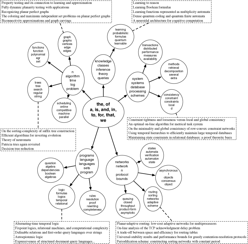
Figure 1. The topic hierarchy learned from 536 abstracts of the Journal of the ACM (JACM) from 1987–2004. The vocabulary was restricted to the 1,539 terms that occurred in more than five documents, yielding a corpus of 68K words. The learned hierarchy contains 25 topics, and each topic node is annotated with its top five most probable terms. We also present examples of documents associated with a subset of the paths in the hierarchy.

The input corpus in this case was a collection of abstracts from the Journal of the ACM (JACM) from the years 1987 to 2004. The figure depicts a topology that is given highest probability by our algorithm, along with the highest probability words from the topics associated with this topology (each node in the tree corresponds to a single topic). As can be seen from the figure, the algorithm has discovered the category of function words at level zero (e.g., “the” and “of”), and has discovered a set of first-level topics that are a reasonably faithful representation of some of the main areas of computer science. The second level provides a further subdivision into more concrete topics. We emphasize that this is an unsupervised problem. The algorithm discovers the topic hierarchy without any extra information about the corpus (e.g., keywords, titles or authors). The documents are the only inputs to the algorithm.

A learned topic hierarchy can be useful for many tasks, including text categorization, text compression, text summarization and language modeling for speech recognition. A commonly-used surrogate for the evaluation of performance in these tasks is predictive likelihood, and we use predictive likelihood to evaluate our methods quantitatively. But we also view our work as making a contribution to the development of methods for the visualization and browsing of documents. The model and algorithm we describe can be used to build a topic hierarchy for a document collection, and that hierarchy can be used to sharpen a user’s understanding of the contents of the collection. A qualitative measure of the success of our approach is that the same tool should be able to uncover a useful topic hierarchy in different domains based solely on the input data.

By defining a probabilistic model for documents, we do not define the level of “abstraction” of a topic formally, but rather define a statistical procedure that allows a system designer to capture notions of abstraction that are reflected in usage patterns of the specific corpus at hand. While the content of topics will vary across corpora, the ways in which abstraction interacts with usage will not. A corpus might be a collection of images, a collection of HTML documents or a collection of DNA sequences. Different notions of abstraction will be appropriate in these different domains, but each are expressed and discoverable in the data, making it possible to automatically construct a hierarchy of topics.

This paper is organized as follows. We begin with a review of the necessary background in stochastic processes and Bayesian nonparametric statistics in Section 2. In Section 3, we develop the nested Chinese restaurant process, the prior on topologies that we use in the hierarchical topic model of Section 4. We derive an approximate posterior inference algorithm in Section 5 to learn topic hierarchies from text data. Examples and an empirical evaluation are provided in Section 6. Finally, we present related work and a discussion in Section 7.

2. Background

Our approach to topic modeling reposes on several building blocks from stochastic process theory and Bayesian nonparametric statistics, specifically the Chinese restaurant process (Aldous, 1985), stick-breaking processes (Pitman, 2002), and the Dirichlet process mixture (Antoniak, 1974). In this section we briefly review these ideas and the connections between them.

2.1. Dirichlet and beta distributions

Recall that the Dirichlet distribution is a probability distribution on the simplex of nonnegative real numbers that sum to one. We write

$$U\sim\textrm{Dir}(\alpha_{1},\alpha_{2},\ldots,\alpha_{K}),$$

for a random vector $U$ distributed as a Dirichlet random variable on the $K$-simplex, where $\alpha_{i}>0$ are parameters. The mean of $U$ is proportional to the parameters

$$E[U_{i}]=\frac{\alpha_{i}}{\sum_{k=1}^{K}\alpha_{k}}$$

and the magnitude of the parameters determines the concentration of $U$ around the mean. The specific choice $\alpha_{1}=\cdots=\alpha_{K}=1$ yields the uniform distribution on the simplex. Letting $\alpha_{i}>1$ yields a unimodal distribution peaked around the mean, and letting $\alpha_{i}<1$ yields a distribution that has modes at the corners of the simplex. The beta distribution is a special case of the Dirichlet distribution for $K=2$, in which case the simplex is the unit interval $(0,1)$. In this case we write $U\sim\textrm{Beta}(\alpha_{1},\alpha_{2})$, where $U$ is a scalar.

2.2. Chinese restaurant process

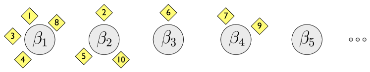
Figure 2. A configuration of the Chinese restaurant process. There are an infinite number of tables, each associated with a parameter $\beta_{i}$. The customers sit at the tables according to Eq. (1) and each generate data with the corresponding parameter. In this configuration, ten customers have been seated in the restaurant, populating four of the infinite set of tables.

The Chinese restaurant process (CRP) is a single parameter distribution over partitions of the integers. The distribution can be most easily described by specifying how to draw a sample from it. Consider a restaurant with an infinite number of tables each with infinite capacity. A sequence of $N$ customers arrive, labeled with the integers $\{1,\ldots,N\}$. The first customer sits at the first table; the $n$th subsequent customer sits at a table drawn from the following distribution:

(1) $$\begin{array}[]{rcl}p(\textrm{occupied table $i$}\,|\,\textrm{previous customers})&=&\frac{n_{i}}{\gamma+n-1}\\ p(\textrm{next unoccupied table}\,|\,\textrm{previous customers})&=&\frac{\gamma}{\gamma+n-1},\end{array}$$

where $n_{i}$ is the number of customers currently sitting at table $i$, and $\gamma$ is a real-valued parameter which controls how often, relative to the number of customers in the restaurant, a customer chooses a new table versus sitting with others. After $N$ customers have been seated, the seating plan gives a partition of those customers as illustrated in Figure 2.

With an eye towards Bayesian statistical applications, we assume that each table is endowed with a parameter vector $\beta$ drawn from a distribution $G_{0}$. Each customer is associated with the parameter vector at the table at which he sits. The resulting distribution on sequences of parameter values is referred to as a Pólya urn model (Johnson and Kotz, 1977).

The Pólya urn distribution can be used to define a flexible clustering model. Let the parameters at the tables index a family of probability distributions (for example, the distribution might be a multivariate Gaussian in which case the parameter would be a mean vector and covariance matrix). Associate customers to data points, and draw each data point from the probability distribution associated with the table at which the customer sits. This induces a probabilistic clustering of the generated data because customers sitting around each table share the same parameter vector.

This model is in the spirit of a traditional mixture model (Titterington et al., 1985), but is critically different in that the number of tables is unbounded. Data analysis amounts to inverting the generative process to determine a probability distribution on the “seating assignment” of a data set. The underlying CRP lets the data determine the number of clusters (i.e., the number of occupied tables) and further allows new data to be assigned to new clusters (i.e., new tables).

2.3. Stick-breaking constructions

The Dirichlet distribution places a distribution on nonnegative $K$-dimensional vectors whose components sum to one. In this section we discuss a stochastic process that allows $K$ to be unbounded.

Consider a collection of nonnegative real numbers $\{\theta_{i}\}_{i=1}^{\infty}$ where $\sum_{i}\theta_{i}=1$. We wish to place a probability distribution on such sequences. Given that each such sequence can be viewed as a probability distribution on the positive integers, we obtain a distribution on distributions, i.e., a random probability distribution.

To do this, we use a stick-breaking construction. View the interval $(0,1)$ as a unit-length stick. Draw a value $V_{1}$ from a $\textrm{Beta}(\alpha_{1},\alpha_{2})$ distribution and break off a fraction $V_{1}$ of the stick. Let $\theta_{1}=V_{1}$ denote this first fragment of the stick and let $1-\theta_{1}$ denote the remainder of the stick. Continue this procedure recursively, letting $\theta_{2}=V_{2}(1-\theta_{1})$, and in general define

$$\theta_{i}=V_{i}\prod_{j=1}^{i-1}(1-V_{j}),$$

where $\{V_{i}\}$ are an infinite sequence of independent draws from the $\textrm{Beta}(\alpha_{1},\alpha_{2})$ distribution. Sethuraman (1994) shows that the resulting sequence $\{\theta_{i}\}$ satisfies $\sum_{i}\theta_{i}=1$ with probability one.

In the special case $\alpha_{1}=1$ we obtain a one-parameter stochastic process known as the GEM distribution (Pitman, 2002). Let $\gamma=\alpha_{2}$ denote this parameter and denote draws from this distribution as $\theta\sim\textrm{GEM}(\gamma)$. Large values of $\gamma$ skew the beta distribution towards zero and yield random sequences that are heavy-tailed, i.e., significant probability tends to be assigned to large integers. Small values of $\gamma$ yield random sequences that decay more quickly to zero.

2.4. Connections

The GEM distribution and the CRP are closely related. Let $\theta\sim\textrm{GEM}(\gamma)$ and let $\{Z_{1},Z_{2},\ldots,Z_{N}\}$ be a sequence of indicator variables drawn independently from $\theta$, i.e.,

$$p(Z_{n}=i\,|\,\theta)=\theta_{i}.$$

This distribution on indicator variables induces a random partition on the integers $\{1,2,\ldots,N\}$, where the partition reflects indicators that share the same values. It can be shown that this distribution on partitions is the same as the distribution on partitions induced by the CRP (Pitman, 2002). As implied by this result, the GEM parameter $\gamma$ controls the partition in the same way as the CRP parameter $\gamma$.

As with the CRP, we can augment the GEM distribution to consider draws of parameter values. Let $\{\beta_{i}\}$ be an infinite sequence of independent draws from a distribution $G_{0}$ defined on a sample space $\Omega$. Define

$$G=\sum_{i=1}^{\infty}\theta_{i}\delta_{\beta_{i}},$$

where $\delta_{\beta_{i}}$ is an atom at location $\beta_{i}$ and where $\theta\sim\textrm{GEM}(\gamma)$. The object $G$ is a distribution on $\Omega$; it is a random distribution.

Consider now a finite partition of $\Omega$. Sethuraman (1994) showed that the probability assigned by $G$ to the cells of this partition follows a Dirichlet distribution. Moreover, if we consider all possible finite partitions of $\Omega$, the resulting Dirichlet distributions are consistent with each other. Thus, by appealing to the Kolmogorov consistency theorem (Billingsley, 1995), we can view $G$ as a draw from an underlying stochastic process, where the index set is the set of Borel sets of $\Omega$. This stochastic process is known as the Dirichlet process (Ferguson, 1973).

Note that if we truncate the stick-breaking process after $L-1$ breaks, we obtain a Dirichlet distribution on an $L$-dimensional vector. The first $L-1$ components of this vector manifest the same kind of bias towards larger values for earlier components as the full stick-breaking distribution. However, the last component $\theta_{L}$ represents the portion of the stick that remains after $L-1$ breaks and has less of a bias toward small values than in the untruncated case.

Finally, we will find it convenient to define a two-parameter variant of the GEM distribution that allows control over both the mean and variance of stick lengths. We denote this distribution as $\textrm{GEM}(m,\pi)$, in which $\pi>0$ and $m\in(0,1)$. In this variant, the stick lengths are defined as $V_{i}\sim\textrm{Beta}(m\pi,(1-m)\pi)$. The standard $\textrm{GEM}(\gamma)$ is the special case when $m\pi=1$ and $\gamma=(1-m)\pi$. Note that its mean and variance are tied through its single parameter.

3. The nested Chinese restaurant process

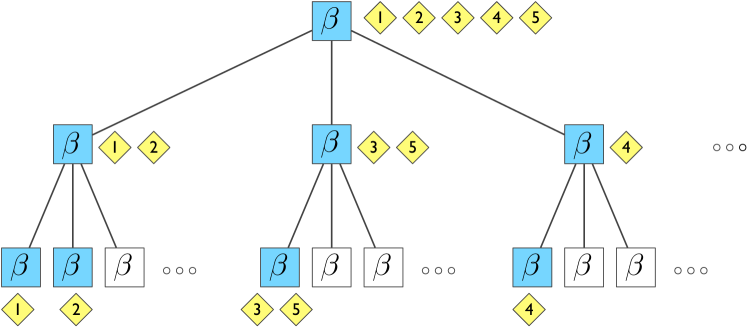
Figure 3. A configuration of the nested Chinese restaurant process illustrated to three levels. Each box represents a restaurant with an infinite number of tables, each of which refers to a unique table in the next level of the tree. In this configuration, five tourists have visited restaurants along four unique paths. Their paths trace a subtree in the infinite tree. (Note that the configuration of customers within each restaurant can be determined by observing the restaurants chosen by customers at the next level of the tree.) In the hLDA model of Section 4, each restaurant is associated with a topic distribution $\beta$. Each document is assumed to choose its words from the topic distributions along a randomly chosen path.

The Chinese restaurant process and related distributions are widely used in Bayesian nonparametric statistics because they make it possible to define statistical models in which observations are assumed to be drawn from an unknown number of classes. However, this kind of model is limited in the structures that it allows to be expressed in data. Analyzing the richly structured data that are common in computer science requires extending this approach. In this section we discuss how similar ideas can be used to define a probability distribution on infinitely-deep, infinitely-branching trees. This distribution is subsequently used as a prior distribution in a hierarchical topic model that identifies documents with paths down the tree.

A tree can be viewed as a nested sequence of partitions. We obtain a distribution on trees by generalizing the CRP to such sequences. Specifically, we define a nested Chinese restaurant process (nCRP) by imagining the following scenario for generating a sample. Suppose there are an infinite number of infinite-table Chinese restaurants in a city. One restaurant is identified as the root restaurant, and on each of its infinite tables is a card with the name of another restaurant. On each of the tables in those restaurants are cards that refer to other restaurants, and this structure repeats infinitely many times. Each restaurant is referred to exactly once; thus, the restaurants in the city are organized into an infinitely-branched, infinitely-deep tree. Note that each restaurant is associated with a level in this tree. The root restaurant is at level 1, the restaurants referred to on its tables’ cards are at level 2, and so on.

A tourist arrives at the city for an culinary vacation. On the first evening, he enters the root Chinese restaurant and selects a table using the CRP distribution in Eq. (1). On the second evening, he goes to the restaurant identified on the first night’s table and chooses a second table using a CRP distribution based on the occupancy pattern of the tables in the second night’s restaurant. He repeats this process forever. After $M$ tourists have been on vacation in the city, the collection of paths describes a random subtree of the infinite tree; this subtree has a branching factor of at most $M$ at all nodes. See Figure 3 for an example of the first three levels from such a random tree.

There are many ways to place prior distributions on trees, and our specific choice is based on several considerations. First and foremost, a prior distribution combines with a likelihood to yield a posterior distribution, and we must be able to compute this posterior distribution. In our case, the likelihood will arise from the hierarchical topic model to be described in Section 4. As we will show in Section 5, the specific prior that we propose in this section combines with the likelihood to yield a posterior distribution that is amenable to probabilistic inference. Second, we have retained important aspects of the CRP, in particular the “preferential attachment” dynamics that are built into Eq. (1). Probability structures of this form have been used as models in a variety of applications (Barabasi and Reka, 1999; Krapivsky and Redner, 2001; Albert and Barabasi, 2002; Drinea et al., 2006), and the clustering that they induce makes them a reasonable starting place for a hierarchical topic model.

In fact, these two points are intimately related. The CRP yields an exchangeable distribution across partitions, i.e., the distribution is invariant to the order of the arrival of customers (Pitman, 2002). This exchangeability property makes CRP-based models amenable to posterior inference using Monte Carlo methods (Escobar and West, 1995; MacEachern and Muller, 1998; Neal, 2000).

4. Hierarchical latent Dirichlet allocation

The nested CRP provides a way to define a prior on tree topologies that does not limit the branching factor or depth of the trees. We can use this distribution as a component of a probabilistic topic model.

The goal of topic modeling is to identify subsets of words that tend to co-occur within documents. Some of the early work on topic modeling derived from latent semantic analysis, an application of the singular value decomposition in which “topics” are viewed post hoc as the basis of a low-dimensional subspace (Deerwester et al., 1990). Subsequent work treated topics as probability distributions over words and used likelihood-based methods to estimate these distributions from a corpus (Hofmann, 1999b). In both of these approaches, the interpretation of “topic” differs in key ways from the clustering metaphor because the same word can be given high probability (or weight) under multiple topics. This gives topic models the capability to capture notions of polysemy (e.g., “bank” can occur with high probability in both a finance topic and a waterways topic). Probabilistic topic models were given a fully Bayesian treatment in the latent Dirichlet allocation (LDA) model (Blei et al., 2003).

Topic models such as LDA treat topics as a “flat” set of probability distributions, with no direct relationship between one topic and another. While these models can be used to recover a set of topics from a corpus, they fail to indicate the level of abstraction of a topic, or how the various topics are related. The model that we present in this section builds on the nCRP to define a hierarchical topic model. This model arranges the topics into a tree, with the desideratum that more general topics should appear near the root and more specialized topics should appear near the leaves (Hofmann, 1999a). Having defined such a model, we use probabilistic inference to simultaneously identify the topics and the relationships between them.

Our approach to defining a hierarchical topic model is based on identifying documents with the paths generated by the nCRP. We augment the nCRP in two ways to obtain a generative model for documents. First, we associate a topic, i.e., a probability distribution across words, with each node in the tree. A path in the tree thus picks out an infinite collection of topics. Second, given a choice of path, we use the GEM distribution to define a probability distribution on the topics along this path. Given a draw from a GEM distribution, a document is generated by repeatedly selecting topics according to the probabilities defined by that draw, and then drawing each word from the probability distribution defined by its selected topic.

More formally, consider the infinite tree defined by the nCRP and let $\textbf{c}_{d}$ denote the path through that tree for the $d$th customer (i.e., document). In the hierarchical LDA (hLDA) model, the documents in a corpus are assumed drawn from the following generative process:

1. For each table $k\in{\cal T}$ in the infinite tree,

   1. Draw a topic $\beta_{k}\sim\textrm{Dirichlet}(\eta)$.

2. For each document, $d\in\{1,2,\ldots,D\}$

   1. Draw $\textbf{c}_{d}\sim\textrm{nCRP}(\gamma)$.

   2. Draw a distribution over levels in the tree, $\theta_{d}\,|\,\{m,\pi\}\sim\textrm{GEM}(m,\pi)$.

   3. For each word,

      1. Choose level $Z_{d,n}\,|\,\theta\sim\textrm{Mult}(\theta_{d})$.

      2. Choose word $W_{d,n}\,|\,\{z_{d,n},\textbf{c}_{d},\mathbold{\beta}\}\sim\textrm{Mult}(\beta_{\textbf{c}_{d}}[z_{d,n}])$, which is parameterized by the topic in position $z_{d,n}$ on the path $\textbf{c}_{d}$.

This generative process defines a probability distribution across possible corpora.

The goal of finding a topic hierarchy at different levels of abstraction is distinct from the problem of hierarchical clustering Zamir and Etzioni (1998); Larsen and Aone (1999); Vaithyanathan and Dom (2000); Duda et al. (2000); Hastie et al. (2001); Heller and Ghahramani (2005). Hierarchical clustering treats each data point as a leaf in a tree, and merges similar data points up the tree until all are merged into a root node. Thus, internal nodes represent summaries of the data below which, in this setting, would yield distributions across words that share high probability words with their children.

In the hierarchical topic model, the internal nodes are not summaries of their children. Rather, the internal nodes reflect the shared terminology of the documents assigned to the paths that contain them. This can be seen in Figure 1, where the high probability words of a node are distinct from the high probability words of its children.

It is important to emphasize that our approach is an unsupervised learning approach in which the probabilistic components that we have defined are latent variables. That is, we do not assume that topics are predefined, nor do we assume that the nested partitioning of documents or the allocation of topics to levels are predefined. We infer these entities from a Bayesian computation in which a posterior distribution is obtained from conditioning on a corpus and computing probabilities for all latent variables.

As we will see experimentally, there is statistical pressure in the posterior to place more general topics near the root of the tree and to place more specialized topics further down in the tree. To see this, note that each path in the tree includes the root node. Given that the GEM distribution tends to assign relatively large probabilities to small integers, there will be a relatively large probability for documents to select the root node when generating words. Therefore, to explain an observed corpus, the topic at the root node will place high probability on words that are useful across all the documents.

Moving down in the tree, recall that each document is assigned to a single path. Thus, the first level below the root induces a coarse partition on the documents, and the topics at that level will place high probability on words that are useful within the corresponding subsets. As we move still further down, the nested partitions of documents become finer. Consequently, the corresponding topics will be more specialized to the particular documents in those paths.

We have presented the model as a two-phase process: an infinite set of topics are generated and assigned to all of the nodes of an infinite tree, and then documents are obtained by selecting nodes in the tree and drawing words from the corresponding topics. It is also possible, however, to conceptualize a “lazy” procedure in which a topic is generated only when a node is first selected. In particular, consider an empty tree (i.e., containing no topics) and consider generating the first document. We select a path and then repeatedly select nodes along that path in order to generate words. A topic is generated at a node when that node is first selected and subsequent selections of the node reuse the same topic.

After $n$ words have been generated, at most $n$ nodes will have been visited and at most $n$ topics will have been generated. The $(n+1)$th word in the document can come from one of previously generated topics or it can come from a new topic. Similarly, suppose that $d$ documents have previously been generated. The $(d+1)$th document can follow one of the paths laid down by an earlier document and select only “old” topics, or it can branch off at any point in the tree and generated “new” topics along the new branch.

This discussion highlights the nonparametric nature of our model. Rather than describing a corpus by using a probabilistic model involving a fixed set of parameters, our model assumes that the number of parameters can grow as the corpus grows, both within documents and across documents. New documents can spark new subtopics or new specializations of existing subtopics. Given a corpus, this flexibility allows us to use approximate posterior inference to discover the particular tree of topics that best describes its documents.

It is important to note that even with this flexibility, the model still makes assumptions about the tree. Its size, shape, and character will be affected by the settings of the hyperparameters. The most influential hyperparameters in this regard are the Dirichlet parameter for the topics $\eta$ and the stick-breaking parameters for the topic proportions $\{m,\pi\}$. The Dirichlet parameter controls the sparsity of the topics; smaller values of $\eta$ will lead to topics with most of their probability mass on a small set of words. With a prior bias to sparser topics, the posterior will prefer more topics to describe a collection and thus place higher probability on larger trees. The stick-breaking parameters control how many words in the documents are likely to come from topics of varying abstractions. If we set $\pi$ to be large (e.g., $\pi=0.5$) then the posterior will more likely assign more words from each document to higher levels of abstraction. Setting $m$ to be large (e.g., $m=100$) means that word allocations will not likely deviate from such a setting.

How we set these hyperparameters depends on the goal of the analysis. When we analyze a document collection with hLDA for discovering and visualizing a hierarchy embedded within it, we might examine various settings of the hyperparameters to find a tree that meets our exploratory needs. We analyze documents with this purpose in mind in Section 6.2. In a different setting, when we are looking for a good predictive model of the data, e.g., to compare hLDA to other statistical models of text, then it makes sense to “fit” the hyperparameters by placing priors on them and computing their posterior. We describe posterior inference for the hyperparameters in Section 5.4 and analyze documents using this approach in Section 6.3.

Finally, we note that hLDA is the simplest model that exploits the nested CRP, i.e., a flexible hierarchy of distributions, in the topic modeling framework. In a more complicated model, one could consider a variant of hLDA where each document exhibits multiple paths through the tree. This can be modeled using a two-level distribution for word generation: first choose a path through the tree, and then choose a level for the word.

Recent extensions to topic models can also be adapted to make use of a flexible topic hierarchy. As examples, in the dynamic topic model the documents are time stamped and the underlying topics change over time (Blei and Lafferty, 2006); in the author-topic model the authorship of the documents affects which topics they exhibit (Rosen-Zvi et al., 2004). This said, some extensions are more easily adaptable than others. In the correlated topic model, the topic proportions exhibit a covariance structure (Blei and Lafferty, 2007). This is achieved by replacing a Dirichlet distribution with a logistic normal, and the application of Bayesian nonparametric extensions is less direct.

4.1. Related work

In previous work, researchers have developed a number of methods that employ hierarchies in analyzing text data. In one line of work, the algorithms are given a hierarchy of document categories, and their goal is to correctly place documents within it (Koller and Sahami, 1997; Chakrabarti et al., 1998; McCallum et al., 1999; Dumais and Chen, 2000). Other work has focused on deriving hierarchies of individual terms using side information, such as a grammar or a thesaurus, that are sometimes available for text domains (Sanderson and Croft, 1999; Stoica and Hearst, 2004; Cimiano et al., 2005).

Our method provides still another way to employ a notion of hierarchy in text analysis. First, rather than learn a hierarchy of terms we learn a hierarchy of topics, where a topic is a distribution over terms that describes a significant pattern of word co-occurrence in the data. Moreover, while we focus on text, a “topic” is simply a data-generating distribution; we do not rely on any text-specific side information such as a thesaurus or grammar. Thus, by using other data types and distributions, our methodology is readily applied to biological data sets, purchasing data, collections of images, or social network data. (Note that applications in such domains have already been demonstrated for flat topic models (Pritchard et al., 2000; Marlin, 2003; Fei-Fei and Perona, 2005; Blei and Jordan, 2003; Airoldi et al., 2008).) Finally, as a Bayesian nonparametric model, our approach can accommodate future data that might lie in new and previously undiscovered parts of the tree. Previous work commits to a single fixed tree for all future data.

5. Probabilistic inference

With the hLDA model in hand, our goal is to perform posterior inference, i.e., to “invert” the generative process of documents described above for estimating the hidden topical structure of a document collection. We have constructed a joint distribution of hidden variables and observations—the latent topic structure and observed documents—by combining prior expectations about the kinds of tree topologies we will encounter with a generative process for producing documents given a particular topology. We are now interested in the distribution of the hidden structure conditioned on having seen the data, i.e., the distribution of the underlying topic structure that might have generated an observed collection of documents. Finding this posterior distribution for different kinds of data and models is a central problem in Bayesian statistics. See  Bernardo and Smith (1994) and Gelman et al. (1995) for general introductions to Bayesian statistics.

In our nonparametric setting, we must find a posterior distribution on countably infinite collections of objects—hierarchies, path assignments, and level allocations of words—given a collection of documents. Moreover, we need to be able to do this using the finite resources of the computer. Not surprisingly, the posterior distribution for hLDA is not available in closed form. We must appeal to an approximation.

We develop a Markov chain Monte Carlo (MCMC) algorithm to approximate the posterior for hLDA. In MCMC, one samples from a target distribution on a set of variables by constructing a Markov chain that has the target distribution as its stationary distribution (Robert and Casella, 2004). One then samples from the chain for sufficiently long that it approaches the target, collects the sampled states thereafter, and uses those collected states to estimate the target. This approach is particularly straightforward to apply to latent variable models, where we take the state space of the Markov chain to be the set of values that the latent variables can take on, and the target distribution is the conditional distribution of these latent variables given the observed data.

The particular MCMC algorithm that we present in this paper is a Gibbs sampling algorithm (Geman and Geman, 1984; Gelfand and Smith, 1990). In a Gibbs sampler each latent variable is iteratively sampled conditioned on the observations and all the other latent variables. We employ collapsed Gibbs sampling (Liu, 1994), in which we marginalize out some of the latent variables to speed up the convergence of the chain. Collapsed Gibbs sampling for topic models (Griffiths and Steyvers, 2004) has been widely used in a number of topic modeling applications (McCallum et al., 2004; Rosen-Zvi et al., 2004; Mimno and McCallum, 2007; Dietz et al., 2007; Newman et al., 2006).

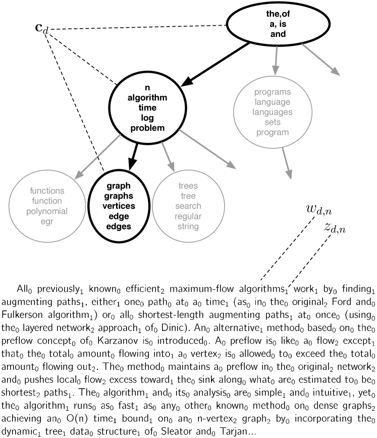
Figure 4. A single state of the Markov chain in the Gibbs sampler for the abstract of “A new approach to the maximum-flow problem” [Goldberg and Tarjan, 1986]. The document is associated with a path through the hierarchy $\textbf{c}_{d}$, and each node in the hierarchy is associated with a distribution over terms. (The five most probable terms are illustrated.) Finally, each word in the abstract $w_{d,n}$ is associated with a level in the path through the hierarchy $z_{d,n}$, with $0$ being the highest level and $2$ being the lowest. The Gibbs sampler iteratively draws $\textbf{c}_{d}$ and $z_{d,n}$ for all words in all documents (see Section 5).

In hLDA, we sample the per-document paths $\textbf{c}_{d}$ and the per-word level allocations to topics in those paths $z_{d,n}$. We marginalize out the topic parameters $\beta_{i}$ and the per-document topic proportions $\theta_{d}$. The state of the Markov chain is illustrated, for a single document, in Figure 4. (The particular assignments illustrated in the figure are taken at the approximate mode of the hLDA model posterior conditioned on abstracts from the JACM.)

Thus, we approximate the posterior $p(\textbf{c}_{1:D},\textbf{z}_{1:D}\,|\,\gamma,\eta,m,\pi,\textbf{w}_{1:D})$. The hyperparameter $\gamma$ reflects the tendency of the customers in each restaurant to share tables, $\eta$ reflects the expected variance of the underlying topics (e.g, $\eta\ll 1$ will tend to choose topics with fewer high-probability words), and $m$ and $\pi$ reflect our expectation about the allocation of words to levels within a document. The hyperparameters can be fixed according to the constraints of the analysis and prior expectation about the data, or inferred as described in Section 5.4.

Intuitively, the CRP parameter $\gamma$ and topic prior $\eta$ provide control over the size of the inferred tree. For example, a model with large $\gamma$ and small $\eta$ will tend to find a tree with more topics. The small $\eta$ encourages fewer words to have high probability in each topic; thus, the posterior requires more topics to explain the data. The large $\gamma$ increases the likelihood that documents will choose new paths when traversing the nested CRP.

The GEM parameter $m$ reflects the proportion of general words relative to specific words, and the GEM parameter $\pi$ reflects how strictly we expect the documents to adhere to these proportions. A larger value of $\pi$ enforces the notions of generality and specificity that lead to more interpretable trees.

The remainder of this section is organized as follows. First, we outline the two main steps in the algorithm: the sampling of level allocations and the sampling of path assignments. We then combine these steps into an overall algorithm. Next, we present prior distributions for the hyperparameters of the model and describe posterior inference for the hyperparameters. Finally, we outline how to assess the convergence of the sampler and approximate the mode of the posterior distribution.

5.1. Sampling level allocations

Given the current path assignments, we need to sample the level allocation variable $z_{d,n}$ for word $n$ in document $d$ from its distribution given the current values of all other variables:

(2) $$p(z_{d,n}\,|\,\textbf{z}_{-(d,n)},\textbf{c},\textbf{w},m,\pi,\eta)\propto p(z_{d,n}\,|\,\textbf{z}_{d,-n},m,\pi)p(w_{d,n}\,|\,\textbf{z},\textbf{c},\textbf{w}_{-(d,n)},\eta),$$

where $\textbf{z}_{-(d,n)}$ and $\textbf{w}_{-(d,n)}$ are the vectors of level allocations and observed words leaving out $z_{d,n}$ and $w_{d,n}$ respectively. We will use similar notation whenever items are left out from an index set; for example, $\textbf{z}_{d,-n}$ denotes the level allocations in document $d$, leaving out $z_{d,n}$.

The first term in Eq. (2) is a distribution over levels. This distribution has an infinite number of components, so we sample in stages. First, we sample from the distribution over the space of levels that are currently represented in the rest of the document, i.e., $\max(\textbf{z}_{d,-n})$, and a level deeper than that level. The first components of this distribution are, for $k\leq\max(\textbf{z}_{d,-n})$,

$$p(z_{d,n}=k\,|\,\textbf{z}_{d,-n},m,\pi) = \textrm{E}\left[V_{k}\prod_{j=1}^{k-1}V_{j}\,|\,\textbf{z}_{d,-n},m,\pi\right]$$

$$= \textrm{E}[V_{k}\,|\,\textbf{z}_{d,-n},m,\pi]\prod_{j=1}^{k-1}\textrm{E}[1-V_{j}\,|\,\textbf{z}_{d,-n},m,\pi]$$

$$= \frac{(1-m)\pi+\#[\textbf{z}_{d,-n}=k]}{\pi+\#[\textbf{z}_{d,-n}\geq k]}\prod_{j=1}^{k-1}\frac{m\pi+\#[\textbf{z}_{d,-n}>j]}{\pi+\#[\textbf{z}_{d,-n}\geq j]}$$

where $\#[\cdot]$ counts the elements of an array satisfying a given condition.

The second term in Eq. (2) is the probability of a given word based on a possible assignment. From the assumption that the topic parameters $\beta_{i}$ are generated from a Dirichlet distribution with hyperparameters $\eta$ we obtain

(3) $$p(w_{d,n}\,|\,\textbf{z},\textbf{c},\textbf{w}_{-(d,n)},\eta)\propto\#[\textbf{z}_{-(d,n)}=z_{d,n},\textbf{c}_{z_{d,n}}=c_{d,z_{d,n}},\textbf{w}_{-(d,n)}=w_{d,n}]+\eta$$

which is the smoothed frequency of seeing word $w_{d,n}$ allocated to the topic at level $z_{d,n}$ of the path ${\bf c}_{d}$.

The last component of the distribution over topic assignments is

$$p(z_{d,n}>\max(\textbf{z}_{d,-n})\,|\,\textbf{z}_{d,-n},\textbf{w},m,\pi,\eta)=1-\sum_{j=1}^{\max(\textbf{z}_{d,-n})}p(z_{d,n}=j\,|\,\textbf{z}_{d,-n},\textbf{w},m,\pi,\eta).$$

If the last component is sampled then we sample from a Bernoulli distribution for increasing values of $\ell$, starting with $\ell=\max(\textbf{z}_{d,-n})+1$, until we determine $z_{d,n}$,

$$p(z_{d,n}=\ell\,|\,z_{d,-n},z_{d,n}>\ell-1,\textbf{w},m,\pi,\eta) = (1-m)p(w_{d,n}\,|\,\textbf{z},\textbf{c},\textbf{w}_{-(d,n)},\eta)$$

$$p(z_{d,n}>\ell\,|\,z_{d,-n},z_{d,n}>\ell-1) = 1-p(z_{d,n}=\ell\,|\,z_{d,-n},z_{d,n}>\ell-1,\textbf{w},m,\pi,\eta).$$

Note that this changes the maximum level when resampling subsequent level assignments.

5.2. Sampling paths

Given the level allocation variables, we need to sample the path associated with each document conditioned on all other paths and the observed words. We appeal to the fact that $\max(\textbf{z}_{d})$ is finite, and are only concerned with paths of that length:

(4) $$p(\textbf{c}_{d}\,|\,\textbf{w},\textbf{c}_{-d},\textbf{z},\eta,\gamma)\propto p(\textbf{c}_{d}\,|\,\textbf{c}_{-d},\gamma)p(\textbf{w}_{d}\,|\,\textbf{c},\textbf{w}_{-d},\textbf{z},\eta).$$

This expression is an instance of Bayes’s theorem with $p(\textbf{w}_{d}\,|\,\textbf{c},\textbf{w}_{-d},\textbf{z},\eta)$ as the probability of the data given a particular choice of path, and $p(\textbf{c}_{d}\,|\,\textbf{c}_{-d},\gamma)$ as the prior on paths implied by the nested CRP. The probability of the data is obtained by integrating over the multinomial parameters, which gives a ratio of normalizing constants for the Dirichlet distribution,

$$\begin{split}&p(\textbf{w}_{d}\,|\,\textbf{c},\textbf{w}_{-d},\textbf{z},\eta)=\\ &\prod_{\ell=1}^{\max(\textbf{z}_{d})}\frac{\Gamma\left(\textstyle\sum_{w}\#[\textbf{z}_{-d}=\ell,\textbf{c}_{-d,\ell}=c_{d,\ell},\textbf{w}_{-d}=w]+V\eta\right)}{\prod_{w}\Gamma\left(\#[\textbf{z}_{-d}=\ell,\textbf{c}_{-d,\ell}=c_{d,\ell},\textbf{w}_{-d}=w]+\eta\right)}\frac{\prod_{w}\Gamma\left(\#[\textbf{z}=\ell,\textbf{c}_{\ell}=c_{d,\ell},\textbf{w}=w]+\eta\right)}{\Gamma\left(\textstyle\sum_{w}\#[\textbf{z}=\ell,\textbf{c}_{\ell}=c_{d,\ell},\textbf{w}=w]+V\eta\right)},\end{split}$$

where we use the same notation for counting over arrays of variables as above. Note that the path must be drawn as a block, because its value at each level depends on its value at the previous level. The set of possible paths corresponds to the union of the set of existing paths through the tree, each represented by a leaf, with the set of possible novel paths, each represented by an internal node.

5.3. Summary of Gibbs sampling algorithm

With these conditional distributions in hand, we specify the full Gibbs sampling algorithm. Given the current state of the sampler, $\{\textbf{c}^{(t)}_{1:D},\textbf{z}^{(t)}_{1:D}\}$, we iteratively sample each variable conditioned on the rest.

1. For each document $d\in\{1,\ldots,D\}$

   1. Randomly draw $\textbf{c}_{d}^{(t+1)}$ from Eq. (4).

   2. Randomly draw $z_{n,d}^{(t+1)}$ from Eq. (2) for each word, $n\in\{1,\ldots N_{d}\}$.

The stationary distribution of the corresponding Markov chain is the conditional distribution of the latent variables in the hLDA model given the corpus. After running the chain for sufficiently many iterations that it can approach its stationary distribution (the “burn-in”) we can collect samples at intervals selected to minimize autocorrelation, and approximate the true posterior with the corresponding empirical distribution.

Although this algorithm is guaranteed to converge in the limit, it is difficult to say something more definitive about the speed of the algorithm independent of the data being analyzed. In hLDA, we sample a leaf from the tree for each document $\textbf{c}_{d}$ and a level assignment for each word $z_{d,n}$. As described above, the number of items from which each is sampled depends on the current state of the hierarchy and other level assignments in the document. Two data sets of equal size may induce different trees and yield different running times for each iteration of the sampler. For the corpora analyzed below in Section 6.2, the Gibbs sampler averaged 0.001 seconds per document for the JACM data and Psychological Review data, and 0.006 seconds per document for the Proceedings of the National Academy of Sciences data.

5.4. Sampling the hyperparameters

The values of hyperparameters are generally unknown a priori. We include them in the inference process by endowing them with prior distributions,

$$m \sim \textrm{Beta}(\alpha_{1},\alpha_{2})$$

$$\pi \sim \textrm{Exponential}(\alpha_{3})$$

$$\gamma \sim \textrm{Gamma}(\alpha_{4},\alpha_{5})$$

$$\eta \sim \textrm{Exponential}(\alpha_{6}).$$

These priors also contain parameters (“hyper-hyperparameters”), but the resulting inferences are less influenced by these hyper-hyperparameters than they are by fixing the original hyperparameters to specific values Bernardo and Smith (1994).

To incorporate this extension into the Gibbs sampler, we interleave Metropolis-Hastings (MH) steps between iterations of the Gibbs sampler to obtain new values of $m$, $\pi$, $\gamma$, and $\eta$. This preserves the integrity of the Markov chain, although it may mix slower than the collapsed Gibbs sampler without the MH updates (Robert and Casella, 2004).

5.5. Assessing convergence and approximating the mode

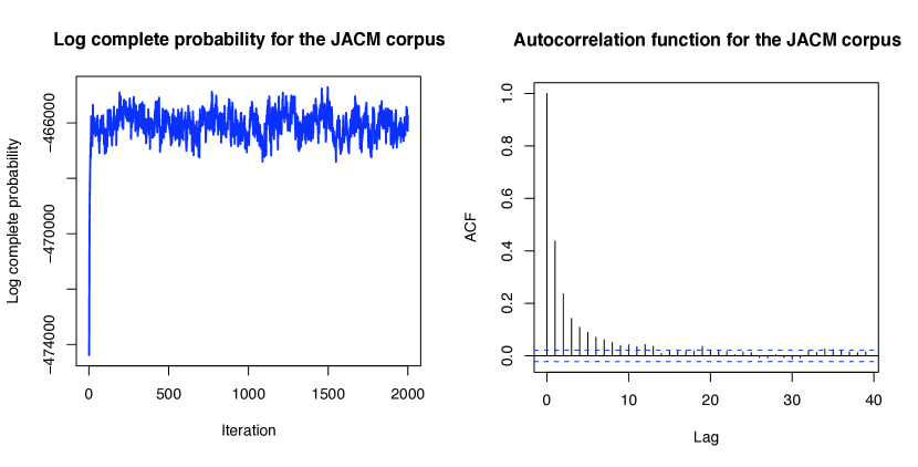
Figure 5. (Left) The complete log likelihood of Eq. (5) for the first 2000 iterations of the Gibbs sampler run on the JACM corpus of Section 6.2. (Right) The autocorrelation function (ACF) of the log complete log likelihood (with confidence interval) for the remaining 8000 iterations. The autocorrelation decreases rapidly as a function of the lag between samples.

Practical applications must address the issue of approximating the mode of the distribution on trees and assessing convergence of the Markov chain. We can obtain information about both by examining the log probability of each sampled state. For a particular sample, i.e., a configuration of the latent variables, we compute the log probability of that configuration and observations, conditioned on the hyperparameters:

(5) $${\cal L}^{(t)}=\log p(\textbf{c}^{(t)}_{1:D},\textbf{z}^{(t)}_{1:D},\textbf{w}_{1:D}\,|\,\gamma,\eta,m,\pi).$$

With this statistic, we can approximate the mode of the posterior by choosing the state with the highest log probability. Moreover, we can assess convergence of the chain by examining the autocorrelation of ${\cal L}^{(t)}$. Figure 5 (right) illustrates the autocorrelation as a function of the number of iterations between samples (the “lag”) when modeling the JACM corpus described in Section 6.2. The chain was run for 10,000 iterations; 2000 iterations were discarded as burn-in.

Figure 5 (left) illustrates Eq. (5) for the burn-in iterations. Gibbs samplers stochastically climb the posterior distribution surface to find an area of high posterior probability, and then explore its curvature through sampling. In practice, one usually restarts this procedure a handful of times and chooses the local mode which has highest posterior likelihood (Robert and Casella, 2004).

Despite the lack of theoretical guarantees, Gibbs sampling is appropriate for the kind of data analysis for which hLDA and many other latent variable models are tailored. Rather than try to understand the full surface of the posterior, the goal of latent variable modeling is to find a useful representation of complicated high-dimensional data, and a local mode of the posterior found by Gibbs sampling often provides such a representation. In the next section, we will assess hLDA qualitatively, through visualization of summaries of the data, and quantitatively, by using the latent variable representation to provide a predictive model of text.

6. Examples and empirical results

We present experiments analyzing both simulated and real text data to demonstrate the application of hLDA and its corresponding Gibbs sampler.

6.1. Analysis of simulated data

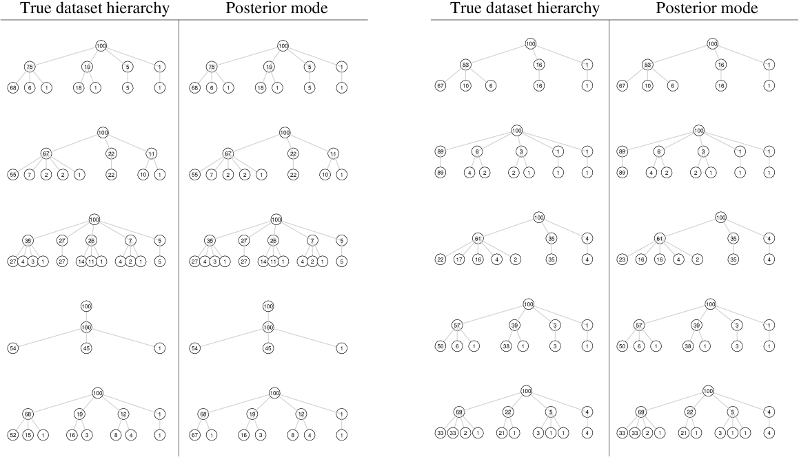
Figure 6. Inferring the mode of the posterior hierarchy from simulated data. See Section 6.1.

In Figure 6, we depict the hierarchies and allocations for ten simulated data sets drawn from an hLDA model. For each data set, we draw 100 documents of 250 words each. The vocabulary size is 100, and the hyperparameters are fixed at $\eta=.005$, and $\gamma=1$. In these simulations, we truncated the stick-breaking procedure at three levels, and simply took a Dirichlet distribution over the proportion of words allocated to those levels. The resulting hierarchies shown in Figure 6 illustrate the range of structures on which the prior assigns probability.

In the same figure, we illustrate the estimated mode of the posterior distribution across the hierarchy and allocations for the ten data sets. We exactly recover the correct hierarchies, with only two errors. In one case, the error is a single wrongly allocated path. In the other case, the inferred mode has higher posterior probability than the true tree structure (due to finite data).

In general we cannot expect to always find the exact tree. This is dependent on the size of the data set, and how identifiable the topics are. Our choice of small $\eta$ yields topics that are relatively sparse and (probably) very different from each other. Trees will not be as easy to identify in data sets which exhibit polysemy and similarity between topics.

6.2. Hierarchy discovery in scientific abstracts

Given a document collection, one is typically interested in examining the underlying tree of topics at the mode of the posterior. As described above, our inferential procedure yields a tree structure by assembling the unique subset of paths contained in $\{\textbf{c}_{1},\ldots,\textbf{c}_{D}\}$ at the approximate mode of the posterior.

For a given tree, we can examine the topics that populate the tree. Given the assignment of words to levels and the assignment of documents to paths, the probability of a particular word at a particular node is roughly proportional to the number of times that word was generated by the topic at that node. More specifically, the mean probability of a word $w$ in a topic at level $\ell$ of path ${\bf p}$ is given by

(6) $$p(w\,|\,\textbf{z},\textbf{c},\textbf{w},\eta)=\frac{\#[\textbf{z}=\ell,\textbf{c}={\bf p},\textbf{w}=w]+\eta}{\#[\textbf{z}=\ell,\textbf{c}={\bf p}]+V\eta}.$$

Using these quantities, the hLDA model can be used for analyzing collections of scientific abstracts, recovering the underlying hierarchical structure appropriate to a collection, and visualizing that hierarchy of topics for a better understanding of the structure of the corpora. We demonstrate the analysis of three different collections of journal abstracts under hLDA.

In these analyses, as above, we truncate the stick-breaking procedure at three levels, facilitating visualization of the results. The topic Dirichlet hyperparameters were fixed at $\eta=\{2.0,1.0,0.5\}$, which encourages many terms in the high-level distributions, fewer terms in the mid-level distributions, and still fewer terms in the low-level distributions. The nested CRP parameter $\gamma$ was fixed at 1.0. The GEM parameters were fixed at $m=100$ and $\pi=0.5$. This strongly biases the level proportions to place more mass at the higher levels of the hierarchy.

In Figure 1, we illustrate the approximate posterior mode of a hierarchy estimated from a collection of 536 abstracts from the JACM. The tree structure illustrates the ensemble of paths assigned to the documents. In each node, we illustrate the top five words sorted by expected posterior probability, computed from Eq. (6). Several leaves are annotated with document titles. For each leaf, we chose the five documents assigned to its path that have the highest numbers of words allocated to the bottom level.

The model has found the function words in the data set, assigning words like “the,” “of,” “or,” and “and” to the root topic. In its second level, the posterior hierarchy appears to have captured some of the major subfields in computer science, distinguishing between databases, algorithms, programming languages and networking. In the third level, it further refines those fields. For example, it delineates between the verification area of networking and the queuing area.

In Figure 7, we illustrate an analysis of a collection of 1,272 psychology abstracts from Psychological Review from 1967 to 2003. Again, we have discovered an underlying hierarchical structure of the field. The top node contains the function words; the second level delineates between large subfields such as behavioral, social and cognitive psychology; the third level further refines those subfields.

Finally, in Figure 8, we illustrate a portion of the analysis of a collection of 12,913 abstracts from the Proceedings of the National Academy of Sciences from 1991 to 2001. An underlying hierarchical structure of the content of the journal has been discovered, dividing articles into groups such as neuroscience, immunology, population genetics and enzymology.

In all three of these examples, the same posterior inference algorithm with the same hyperparameters yields very different tree structures for different corpora. Models of fixed tree structure force us to commit to one in advance of seeing the data. The nested Chinese restaurant process at the heart of hLDA provides a flexible solution to this difficult problem.

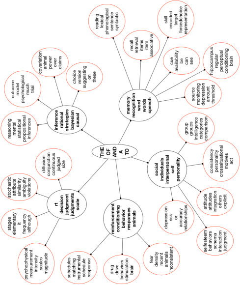
Figure 7. A portion of the hierarchy learned from the 1,272 abstracts of Psychological Review from 1967–2003. The vocabulary was restricted to the 1,971 terms that occurred in more than five documents, yielding a corpus of 136K words. The learned hierarchy, of which only a portion is illustrated, contains 52 topics.

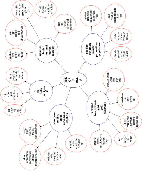
Figure 8. A portion of the hierarchy learned from the 12,913 abstracts of the Proceedings of the National Academy of Sciences from 1991–2001. The vocabulary was restricted to the 7,200 terms that occurred in more than five documents, yielding a corpus of 2.3M words. The learned hierarchy, of which only a portion is illustrated, contains 56 topics. Note that the $\gamma$ parameter is fixed at a smaller value, to provide a reasonably sized topic hierarchy with the significantly larger corpus.

6.3. Comparison to LDA

In this section we present experiments comparing hLDA to its non-hierarchical precursor, LDA. We use the infinite-depth hLDA model; the per-document distribution over levels is not truncated. We use predictive held-out likelihood to compare the two approaches quantitatively, and we present examples of LDA topics in order to provide a qualitative comparison of the methods. LDA has been shown to yield good predictive performance relative to competing unigram language models, and it has also been argued that the topic-based analysis provided by LDA represents a qualitative improvement on competing language models (Blei et al., 2003; Griffiths and Steyvers, 2006). Thus LDA provides a natural point of comparison.

There are several issues that must be borne in mind in comparing hLDA to LDA. First, in LDA the number of topics is a fixed parameter, and a model selection procedure is required to choose the number of topics. (A Bayesian nonparametric solution to this can be obtained with the hierarchical Dirichlet process (Teh et al., 2007).) Second, given a set of topics, LDA places no constraints on the usage of the topics by documents in the corpus; a document can place an arbitrary probability distribution on the topics. In hLDA, on the other hand, a document can only access the topics that lie along a single path in the tree. In this sense, LDA is significantly more flexible than hLDA.

This flexibility of LDA implies that for large corpora we can expect LDA to dominate hLDA in terms of predictive performance (assuming that the model selection problem is resolved satisfactorily and assuming that hyperparameters are set in a manner that controls overfitting). Thus, rather than trying to simply optimize for predictive performance within the hLDA family and within the LDA family, we have instead opted to first run hLDA to obtain a posterior distribution over the number of topics, and then to conduct multiple runs of LDA for a range of topic cardinalities bracketing the hLDA result. This provides an hLDA-centric assessment of the consequences (for predictive performance) of using a hierarchy versus a flat model.

We used predictive held-out likelihood as a measure of performance. The procedure is to divide the corpus into $D_{1}$ observed documents and $D_{2}$ held-out documents, and approximate the conditional probability of the held-out set given the training set

(7) $$p(\textbf{w}^{\textrm{held-out}}_{1},\ldots,\textbf{w}^{\textrm{held-out}}_{D_{2}}\,|\,\textbf{w}^{\textrm{obs}}_{1},\ldots,\textbf{w}^{\textrm{obs}}_{D_{1}},{\cal M}),$$

where ${\cal M}$ represents a model, either LDA or hLDA. We employed collapsed Gibbs sampling for both models and integrated out all the hyperparameters with priors. We used the same prior for those hyperparameters that exist in both models.

To approximate this predictive quantity, we run two samplers. First, we collect 100 samples from the posterior distribution of latent variables given the observed documents, taking samples 100 iterations apart and using a burn-in of 2000 samples. For each of these outer samples, we collect 800 samples of the latent variables given the held-out documents and approximate their conditional probability given the outer sample with the harmonic mean (Kass and Raftery, 1995). Finally, these conditional probabilities are averaged to obtain an approximation to Eq. (7).

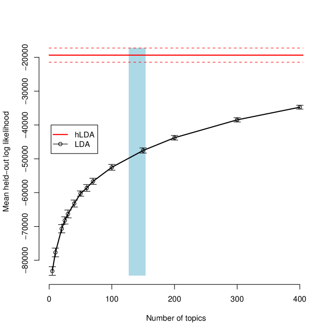
Figure 9. The held-out predictive log likelihood for hLDA compared to the same quantity for LDA as a function of the number of topics. The shaded blue region is centered at the mean number of topics in the hierarchies found by hLDA (and has width equal to twice the standard error).

Figure 10. The five most probable words for each of ten randomly chosen topics from an LDA model fit to fifty topics.

Figure 9 illustrates the five-fold cross-validated held-out likelihood for hLDA and LDA on the JACM corpus. The figure also provides a visual indication of the mean and variance of the posterior distribution over topic cardinality for hLDA; the mode is approximately a hierarchy with 140 topics. For LDA, we plot the predictive likelihood in a range of topics around this value.

We see that at each fixed topic cardinality in this range of topics, hLDA provides significantly better predictive performance than LDA. As discussed above, we eventually expect LDA to dominate hLDA for large numbers of topics. In a large range near the hLDA mode, however, the constraint that documents pick topics along single paths in a hierarchy yields superior performance. This suggests that the hierarchy is useful not only for interpretation, but also for capturing predictive statistical structure.

To give a qualitative sense of the relative degree of interpretability of the topics that are found using the two approaches, Figure 10 illustrates ten LDA topics chosen randomly from a 50-topic model. As these examples make clear, the LDA topics are generally less interpretable than the hLDA topics. In particular, function words are given high probability throughout. In practice, to sidestep this issue, corpora are often stripped of function words before fitting an LDA model. While this is a reasonable ad-hoc solution for (English) text, it is not a general solution that can be used for non-text corpora, such as visual scenes. Even more importantly, there is no notion of abstraction in the LDA topics. The notion of multiple levels of abstraction requires a model such as hLDA.

In summary, if interpretability is the goal, then there are strong reasons to prefer hLDA to LDA. If predictive performance is the goal, then hLDA may well remain the preferred method if there is a constraint that a relatively small number of topics should be used. When there is no such constraint, LDA may be preferred. These comments also suggest, however, that an interesting direction for further research is to explore the feasibility of a model that combines the defining features of the LDA and hLDA models. As we described in Section 4, it may be desirable to consider an hLDA-like hierarchical model that allows each document to exhibit multiple paths along the tree. This might be appropriate for collections of long documents, such as full-text articles, which tend to be more heterogeneous than short abstracts.

7. Discussion

In this paper, we have shown how the nested Chinese restaurant process can be used to define prior distributions on recursive data structures. We have also shown how this prior can be combined with a topic model to yield a Bayesian nonparametric methodology for analyzing document collections in terms of hierarchies of topics. Given a collection of documents, we use MCMC sampling to learn an underlying thematic structure that provides a useful abstract representation for data visualization and summarization.

We emphasize that no knowledge of the topics of the collection or the structure of the tree are needed to infer a hierarchy from data. We have demonstrated our methods on collections of abstracts from three different scientific journals, showing that while the content of these different domains can vary significantly, the statistical principles behind our model make it possible to recover meaningful sets of topics at multiple levels of abstraction, and organized in a tree.

The Bayesian nonparametric framework underlying our work makes it possible to define probability distributions and inference procedures over countably infinite collections of objects. There has been other recent work in artificial intelligence in which probability distributions are defined on infinite objects via concepts from first-order logic (Milch et al., 2005; Pasula and Russell, 2001; Poole, 2007). While providing an expressive language, this approach does not necessarily yield structures that are amenable to efficient posterior inference. Our approach reposes instead on combinatorial structure—the exchangeability of the Dirichlet process as a distribution on partitions—and this leads directly to a posterior inference algorithm that can be applied effectively to large-scale learning problems.

The hLDA model draws on two complementary insights—one from statistics, the other from computer science. From statistics, we take the idea that it is possible to work with general stochastic processes as prior distributions, thus accommodating latent structures that vary in complexity. This is the key idea behind Bayesian nonparametric methods. In recent years, these models have been extended to include spatial models (Duan et al., 2007) and grouped data (Teh et al., 2007), and Bayesian nonparametric methods now enjoy new applications in computer vision (Sudderth et al., 2005), bioinformatics (Xing et al., 2007), and natural language processing (Li et al., 2007; Teh et al., 2007; Goldwater et al., 2006b, a; Johnson et al., 2007; Liang et al., 2007).

From computer science, we take the idea that the representations we infer from data should be richly structured, yet admit efficient computation. This is a growing theme in Bayesian nonparametric research. For example, one line of recent research has explored stochastic processes involving multiple binary features rather than clusters (Griffiths and Ghahramani, 2006; Thibaux and Jordan, 2007; Teh et al., 2007). A parallel line of investigation has explored alternative posterior inference techniques for Bayesian nonparametric models, providing more efficient algorithms for extracting this latent structure. Specifically, variational methods, which replace sampling with optimization, have been developed for Dirichlet process mixtures to further increase their applicability to large-scale data analysis problems (Blei and Jordan, 2005; Kurihara et al., 2007).

The hierarchical topic model that we explored in this paper is just one example of how this synthesis of statistics and computer science can produce powerful new tools for the analysis of complex data. However, this example showcases the two major strengths of the Bayesian nonparametric approach. First, the use of the nested CRP means that the model does not start with a fixed set of topics or hypotheses about their relationship, but grows to fit the data at hand. Thus, we learn a topology but do not commit to it; the tree can grow as new documents about new topics and subtopics are observed. Second, despite the fact that this results in a very rich hypothesis space, containing trees of arbitrary depth and branching factor, it is still possible to perform approximate probabilistic inference using a simple algorithm. This combination of flexible, structured representations and efficient inference makes nonparametric Bayesian methods uniquely promising as a formal framework for learning with flexible data structures.

Acknowledgments

We thank Edo Airoldi for providing the PNAS data, and we thank three anonymous reviewers for their insightful comments. David M. Blei is supported by ONR 175-6343, NSF CAREER 0745520, and grants from Google and Microsoft Research. Thomas L. Griffiths is supported by NSF grant BCS-0631518 and the DARPA CALO project. Michael I. Jordan is supported by grants from Google and Microsoft Research.

References

- Airoldi et al. (2008) Airoldi, E., Blei, D., Fienberg, S., and Xing, E. 2008. Mixed membership stochastic blockmodels. Journal of Machine Learning Research 9, 1981–2014.
- Albert and Barabasi (2002) Albert, R. and Barabasi, A. 2002. Statistical mechanics of complex networks. Reviews of Modern Physics 74, 1, 47–97.
- Aldous (1985) Aldous, D. 1985. Exchangeability and related topics. In École d’Eté de Probabilités de Saint-Flour, XIII—1983. Springer, Berlin, Germany, 1–198.
- Antoniak (1974) Antoniak, C. 1974. Mixtures of Dirichlet processes with applications to Bayesian nonparametric problems. The Annals of Statistics 2, 1152–1174.
- Barabasi and Reka (1999) Barabasi, A. and Reka, A. 1999. Emergence of scaling in random networks. Science 286, 5439, 509–512.
- Bernardo and Smith (1994) Bernardo, J. and Smith, A. 1994. Bayesian Theory. John Wiley & Sons Ltd., Chichester, UK.
- Billingsley (1995) Billingsley, P. 1995. Probability and Measure. Wiley-Interscience, New York, NY.
- Blei et al. (2003) Blei, D., Griffiths, T., Jordan, M., and Tenenbaum, J. 2003. Hierarchical topic models and the nested Chinese restaurant process. In Advances in Neural Information Processing Systems 16. MIT Press, Cambridge, MA, 17–24.
- Blei and Jordan (2003) Blei, D. and Jordan, M. 2003. Modeling annotated data. In Proceedings of the 26th annual International ACM SIGIR Conference on Research and Development in Information Retrieval. ACM Press, 127–134.
- Blei and Jordan (2005) Blei, D. and Jordan, M. 2005. Variational inference for Dirichlet process mixtures. Journal of Bayesian Analysis 1, 121–144.
- Blei and Lafferty (2006) Blei, D. and Lafferty, J. 2006. Dynamic topic models. In Proceedings of the 23rd International Conference on Machine Learning. ACM Press, New York, NY, 113–120.
- Blei and Lafferty (2007) Blei, D. and Lafferty, J. 2007. A correlated topic model of Science. Annals of Applied Statistics 1, 17–35.
- Blei and Lafferty (2009) Blei, D. and Lafferty, J. 2009. Topic models. In Text Mining: Theory and Applications. Taylor and Francis, London, UK.
- Blei et al. (2003) Blei, D., Ng, A., and Jordan, M. 2003. Latent Dirichlet allocation. Journal of Machine Learning Research 3, 993–1022.
- Chakrabarti et al. (1998) Chakrabarti, S., Dom, B., Agrawal, R., and Raghavan, P. 1998. Scalable feature selection, classification and signature generation for organizing large text databases into hierarchical topic taxonomies. The VLDB Journal 7, 163–178.
- Cimiano et al. (2005) Cimiano, P., Hotho, A., and Staab, S. 2005. Learning concept hierarchies from text corpora using formal concept analysis. Journal of Artificial Intelligence Research 24, 305–339.
- Deerwester et al. (1990) Deerwester, S., Dumais, S., Landauer, T., Furnas, G., and Harshman, R. 1990. Indexing by latent semantic analysis. Journal of the American Society of Information Science 6, 391–407.
- Devroye et al. (1996) Devroye, L., Györfi, L., and Lugosi, G. 1996. A Probabilistic Theory of Pattern Recognition. Springer-Verlag, New York, NY.
- Dietz et al. (2007) Dietz, L., Bickel, S., and Scheffer, T. 2007. Unsupervised prediction of citation influences. In Proceedings of the 24th International Conference on Machine Learning. ACM Press, New York, NY, 233–240.
- Drinea et al. (2006) Drinea, E., Enachesu, M., and Mitzenmacher, M. 2006. Variations on random graph models for the web. Tech. Rep. TR-06-01, Harvard University.
- Duan et al. (2007) Duan, J., Guindani, M., and Gelfand, A. 2007. Generalized spatial Dirichlet process models. Biometrika 94, 809–825.
- Duda et al. (2000) Duda, R., Hart, P., and Stork, D. 2000. Pattern Classification. Wiley-Interscience, New York, NY.
- Dumais and Chen (2000) Dumais, S. and Chen, H. 2000. Hierarchical classification of web content. In Proceedings of the 23rd Annual International ACM SIGIR conference on Research and Development in Information Retrieval. ACM Press, New York, NY, 256–263.
- Escobar and West (1995) Escobar, M. and West, M. 1995. Bayesian density estimation and inference using mixtures. Journal of the American Statistical Association 90, 577–588.
- Fei-Fei and Perona (2005) Fei-Fei, L. and Perona, P. 2005. A Bayesian hierarchical model for learning natural scene categories. IEEE Computer Vision and Pattern Recognition, 524–531.
- Ferguson (1973) Ferguson, T. 1973. A Bayesian analysis of some nonparametric problems. Annals of Statistics 1, 209–230.
- Gelfand and Smith (1990) Gelfand, A. and Smith, A. 1990. Sampling based approaches to calculating marginal densities. Journal of the American Statistical Association 85, 398–409.
- Gelman et al. (1995) Gelman, A., Carlin, J., Stern, H., and Rubin, D. 1995. Bayesian Data Analysis. Chapman & Hall, London, UK.
- Geman and Geman (1984) Geman, S. and Geman, D. 1984. Stochastic relaxation, Gibbs distributions and the Bayesian restoration of images. IEEE Transactions on Pattern Analysis and Machine Intelligence 6, 721–741.
- Goldberg and Tarjan (1986) Goldberg, A. and Tarjan, R. 1986. A new approach to the maximum flow problem. Journal of the Association for Computing Machinery 35, 4, 921–940.
- Goldwater et al. (2006a) Goldwater, S., Griffiths, T., and Johnson, M. 2006a. Contextual dependencies in unsupervised word segmentation. In Proceedings of the 21st International Conference on Computational Linguistics and 44th Annual Meeting of the Association for Computational Linguistics. Association for Computational Linguistics, Stroudsburg, PA, 673–680.
- Goldwater et al. (2006b) Goldwater, S., Griffiths, T., and Johnson, M. 2006b. Interpolating between types and tokens by estimating power-law generators. In Advances in Neural Information Processing Systems 18. MIT Press, Cambridge, MA, 459–467.
- Griffiths and Ghahramani (2006) Griffiths, T. and Ghahramani, Z. 2006. Infinite latent feature models and the Indian buffet process. In Advances in Neural Information Processing Systems 18. MIT Press, Cambridge, MA, 475–482.
- Griffiths and Steyvers (2004) Griffiths, T. and Steyvers, M. 2004. Finding scientific topics. Proceedings of the National Academy of Science 101, 5228–5235.
- Griffiths and Steyvers (2006) Griffiths, T. and Steyvers, M. 2006. Probabilistic topic models. In Latent Semantic Analysis: A Road to Meaning, T. Landauer, D. McNamara, S. Dennis, and W. Kintsch, Eds. Erlbaum, Hillsdale, NJ.
- Hastie et al. (2001) Hastie, T., Tibshirani, R., and Friedman, J. 2001. The Elements of Statistical Learning. Springer, New York, NY.
- Heller and Ghahramani (2005) Heller, K. and Ghahramani, Z. 2005. Bayesian hierarchical clustering. In Proceedings of the 22nd International Conference on Machine Learning. ACM Press, Cambridge, MA, 297–304.
- Hjort et al. (2009) Hjort, N., Holmes, C., Müller, P., and Walker, S. 2009. Bayesian Nonparametrics: Principles and Practice. Cambridge University Press, Cambridge, UK.
- Hofmann (1999a) Hofmann, T. 1999a. The cluster-abstraction model: Unsupervised learning of topic hierarchies from text data. In Proceedings of the 15th International Joint Conferences on Artificial Intelligence. Morgan Kaufmann, San Francisco, CA, 682–687.
- Hofmann (1999b) Hofmann, T. 1999b. Probabilistic latent semantic indexing. In Proceedings of the 22nd Annual ACM SIGIR Conference on Research and Development in Information Retrieval. ACM Press, New York, NY, 50–57.
- Johnson et al. (2007) Johnson, M., Griffiths, T., and S., G. 2007. Adaptor grammars: A framework for specifying compositional nonparametric Bayesian models. In Advances in Neural Information Processing Systems 19. MIT Press, Cambridge, MA, 641–648.
- Johnson and Kotz (1977) Johnson, N. and Kotz, S. 1977. Urn Models and Their Applications: An Approach to Modern Discrete Probability Theory. Wiley, New York, NY.
- Jordan (2000) Jordan, M. I. 2000. Graphical models. Statistical Science 19, 140–155.
- Kass and Raftery (1995) Kass, R. and Raftery, A. 1995. Bayes factors. Journal of the American Statistical Association 90, 773–795.
- Koller and Sahami (1997) Koller, D. and Sahami, M. 1997. Hierarchically classifying documents using very few words. In Proceedings of the 14th International Conference on Machine Learning. Morgan Kaufmann, San Francisco, CA, 170–178.
- Krapivsky and Redner (2001) Krapivsky, P. and Redner, S. 2001. Organization of growing random networks. Physical Review E 63, 6.
- Kurihara et al. (2007) Kurihara, K., Welling, M., and Vlassis, N. 2007. Accelerated variational Dirichlet process mixtures. In Advances in Neural Information Processing Systems 19. MIT Press, Cambridge, MA, 761–768.
- Larsen and Aone (1999) Larsen, B. and Aone, C. 1999. Fast and effective text mining using linear-time document clustering. In Proceedings of the 5th ACM SIGKDD International Conference on Knowledge Discovery and Data Mining. ACM Press, New York, NY, 16–22.
- Lauritzen (1996) Lauritzen, S. L. 1996. Graphical Models. Oxford University Press, Oxford, UK.
- Li et al. (2007) Li, W., Blei, D., and McCallum, A. 2007. Nonparametric Bayes pachinko allocation. In Proceedings of the 23rd Conference on Uncertainty in Artificial Intelligence. AUAI Press, Menlo Park, CA.
- Liang et al. (2007) Liang, P., Petrov, S., Klein, D., and Jordan, M. 2007. The infinite PCFG using hierarchical Dirichlet processes. In Proceedings of the 2007 Joint Conference on Empirical Methods in Natural Language Processing and Computational Natural Language Learning. Association for Computational Linguistics, Stroudsburg, PA, 688–697.
- Liu (1994) Liu, J. 1994. The collapsed Gibbs sampler in Bayesian computations with application to a gene regulation problem. Journal of the American Statistical Association 89, 958–966.
- MacEachern and Muller (1998) MacEachern, S. and Muller, P. 1998. Estimating mixture of Dirichlet process models. Journal of Computational and Graphical Statistics 7, 223–238.
- Marlin (2003) Marlin, B. 2003. Modeling user rating profiles for collaborative filtering. In Advances in Neural Information Processing Systems 16. MIT Press, Cambridge, MA, 627–634.
- McCallum et al. (2004) McCallum, A., Corrada-Emmanuel, A., and Wang, X. 2004. The author-recipient-topic model for topic and role discovery in social networks: Experiments with Enron and academic email. Tech. rep., University of Massachusetts, Amherst.
- McCallum et al. (1999) McCallum, A., Nigam, K., Rennie, J., and Seymore, K. 1999. Building domain-specific search engines with machine learning techniques. In Proceedings of the AAAI Spring Symposium on Intelligent Agents in Cyberspace. AAAI Press, Menlo Park, CA.
- Milch et al. (2005) Milch, B., Marthi, B., Sontag, D., Ong, D., and Kobolov, A. 2005. Approximate inference for infinite contingent Bayesian networks. In Proceedings of 10th International Workshop on Artificial Intelligence and Statistics. The Society for Artificial Intelligence and Statistics, NJ.
- Mimno and McCallum (2007) Mimno, D. and McCallum, A. 2007. Organizing the OCA: Learning faceted subjects from a library of digital books. In Proceedings of the 7th ACM/IEEE-CS Joint Conference on Digital libraries. ACM Press, New York, NY, 376–385.
- Neal (2000) Neal, R. 2000. Markov chain sampling methods for Dirichlet process mixture models. Journal of Computational and Graphical Statistics 9, 249–265.
- Newman et al. (2006) Newman, D., Chemudugunta, C., and Smyth, P. 2006. Statistical entity-topic models. In Proceedings of the 12th ACM SIGKDD International Conference on Knowledge Discovery and Data Mining. ACM Press, New York, NY, 680–686.
- Pasula and Russell (2001) Pasula, H. and Russell, S. 2001. Approximate inference for first-order probabilistic languages. In Proceedings of the 17th International Joint Conferences on Artificial Intelligence. Morgan Kaufmann, San Francisco, CA, 741–748.
- Pitman (2002) Pitman, J. 2002. Combinatorial Stochastic Processes. Lecture Notes for St. Flour Summer School. Springer-Verlag, New York, NY.
- Poole (2007) Poole, D. 2007. Logical generative models for probabilistic reasoning about existence, roles and identity. In Proceedings of the 22nd AAAI Conference on Artificial Intelligence. AAAI Press, Menlo Park, CA, 1271–1279.
- Pritchard et al. (2000) Pritchard, J., Stephens, M., and Donnelly, P. 2000. Inference of population structure using multilocus genotype data. Genetics 155, 945–959.
- Robert and Casella (2004) Robert, C. and Casella, G. 2004. Monte Carlo Statistical Methods. Springer-Verlag, New York, NY.
- Rosen-Zvi et al. (2004) Rosen-Zvi, M., Griffiths, T., Steyvers, M., and Smith, P. 2004. The author-topic model for authors and documents. In Proceedings of the 20th Conference on Uncertainty in Artificial Intelligence. AUAI Press, Menlo Park, CA, 487–494.
- Sanderson and Croft (1999) Sanderson, M. and Croft, B. 1999. Deriving concept hierarchies from text. In Proceedings of the 22nd Annual International ACM SIGIR Conference on Research and Development in Information Retrieval. ACM, New York, NY, 206–213.
- Sethuraman (1994) Sethuraman, J. 1994. A constructive definition of Dirichlet priors. Statistica Sinica 4, 639–650.
- Stoica and Hearst (2004) Stoica, E. and Hearst, M. 2004. Nearly-automated metadata hierarchy creation. In Companion Proceedings of HLT-NAACL. Boston, MA.
- Sudderth et al. (2005) Sudderth, E., Torralba, A., Freeman, W., and Willsky, A. 2005. Describing visual scenes using transformed Dirichlet processes. In Advances in Neural Information Processing Systems 18. MIT Press, Cambridge, MA, 1297–1306.
- Teh et al. (2007) Teh, Y., Gorur, D., and Ghahramani, Z. 2007. Stick-breaking construction for the Indian buffet process. In Proceedings of 11th International Workshop on Artificial Intelligence and Statistics. The Society for Artificial Intelligence and Statistics, NJ.
- Teh et al. (2007) Teh, Y., Jordan, M., Beal, M., and Blei, D. 2007. Hierarchical Dirichlet processes. Journal of the American Statistical Association 101, 1566–1581.
- Thibaux and Jordan (2007) Thibaux, R. and Jordan, M. 2007. Hierarchical beta processes and the Indian buffet process. In Proceedings of 11th International Workshop on Artificial Intelligence and Statistics. The Society for Artificial Intelligence and Statistics, NJ.
- Titterington et al. (1985) Titterington, D., Smith, A., and Makov, E. 1985. Statistical Analysis of Finite Mixture Distributions. Wiley, Chichester, UK.
- Vaithyanathan and Dom (2000) Vaithyanathan, S. and Dom, B. 2000. Model-based hierarchical clustering. In Proceedings of the 16th Conference on Uncertainty in Artificial Intelligence. Morgan Kaufmann, San Francisco, CA, 599–608.
- Xing et al. (2007) Xing, E., Jordan, M., and Sharan, R. 2007. Bayesian haplotype inference via the Dirichlet process. Journal of Computational Biology 14, 267–284.
- Zamir and Etzioni (1998) Zamir, O. and Etzioni, O. 1998. Web document clustering: A feasibility demonstration. In Proceedings of the 21st Annual International ACM SIGIR Conference on Research and Development in Information Retrieval. ACM Press, New York, NY, 46–54.