Evidence of random magnetic anisotropy in ferrihydrite nanoparticles based on analysis of statistical distributions

Abstract

We show that the magnetic anisotropy energy of antiferromagnetic ferrihydrite depends on the square root of the nanoparticles volume, using a method based on the analysis of statistical distributions. The size distribution was obtained by transmission electron microscopy, and the anisotropy energy distributions were obtained from ac magnetic susceptibility and magnetic relaxation. The square root dependence corresponds to random local anisotropy, whose average is given by its variance, and can be understood in terms of the recently proposed single phase homogeneous structure of ferrihydrite.

I Introduction

The relation between structural and magnetic properties is of importance from the point of view of applied and fundamental research. This relation is not straightforward in systems with antiferromagnetic (AF) interactions, reduced dimensionality or size such as nanoparticles. In these systems, surface effects and disorder play an important role and therefore deviations to the superparamagnetic (SP) canonic behavior are expected. Such effects change the relation between anisotropy energy, $E_{a}$, volume, $V$, and magnetic moment, $\mu$, found for typical SP systems for which $E_{a}$ and $\mu$ are proportional to $V$. This is also the case of ultrathin films, where anisotropy energy is proportional to surface area, leading to perpendicular magnetization. Important contribution from surface anisotropy is also found in SP nanoparticles with ferromagnetic interactions, where surface atoms constitute a relevant fraction of the total atoms Luis et al. (2002). Another example of non-proportionality between $E_{a}$ and $V$ is two-dimensional Co nanostructures, where $E_{a}$ was found to depend on the perimeter Rusponi et al. (2003).

The deviations to the proportionality between $V$ and $\mu$ found in AF nanoparticles are associated to the fact that, in these systems, the net magnetic moment arises from the uncompensated and/or canted moments, $\mu_{un}$, that can be present at the surface, throughout the volume, or both. The relation between $\mu_{un}$ and $V$ reflect the origin of the moments. In particular, Néel has shown that $\mu_{un}$ is proportional to $V^{q}$ with $q=1/2$ for moments randomly distributed in the volume, $1/3$ for moments randomly distributed in the surface and $2/3$ for moments distributed throughout the surface in active planes Néel (1961). In ferritin, a protein where Fe³⁺ is stored as ferrihydrite, $q$ was estimated to be of the order of $q=1/2$ Makhlouf et al. (1997); Harris et al. (1999) or to be between $1/2$ and $1/3$ Silva et al. (2005) based on magnetization measurements. These values were obtained either by using a system with a given size and estimating the power relation between the total number of ions and the equivalent uncompensated number of ions Makhlouf et al. (1997); Silva et al. (2005), or by the usual comparison of systems with different average sizes Harris et al. (1999). The latter approach is limited by the possibility of synthesizing identical systems with different average volumes, that usually covers less that one order of magnitude. An alternative approach that takes advantage from the size distribution is developed here. A sample with a wide distribution can be regarded as one system containing a set of different average sizes. An approach reminiscent of this approach was first used by Luis and co-workers for the determination of the origin of magnetic anisotropy in gaussian size-distributed Co nanoparticles Luis et al. (2002). They concluded that surface anisotropy has an important contribution, since the $E_{a}$ distribution is narrower than the $V$ distribution. The effect of size distributions on the magnetic properties was later used to study two-dimensional Co structures by Rusponi et al. Rusponi et al. (2003). The idea was based on the fact that the shape of the in-phase component of the ac susceptibility $\chi^{\prime}$ was critically dependent on the chosen distribution, namely surface, perimeter and perimeter plus surface distributions. The authors concluded that perimeter atoms were those relevant to the reversal process in the Co structures, i. e., $E_{a}$ depends on the perimeter. Gilles and co-workers have also tried to use susceptibility curves to obtain the relation between $\mu_{un}$ and $V$ in ferritin Gilles et al. (2000) but found that their experimental curves were not very sensitive to the particular shape of distribution nor the value of $q$ Gilles et al. (2000). In a different context, the luminosity and the size distributions of rare-earth-doped nanoparticles were used to establish the relation between luminosity and size through the size dependent optical detection probability Casanova et al. (2006).

In this report we show that lognormal distributed nanoparticle samples are particularly useful to study the relation between a physical property and size. This is based in the fact that when two physical quantities are related by a power function, the power factor can be readily obtained by comparing the respective lognormal deviations, due to reproductive properties of the lognormal distribution function Crow and Shimizu (1988). Moreover we generalize this concept to any distribution function. This method is of general use and can be simply applied in cases where the size of the system determined a given physical property by a power law relation, as in the optical properties of quantum dots Brus (1986). In the present context of magnetism, we apply this approach to AF ferrihydrite nanoparticles grown in a hybrid matrix to investigate the relation between $E_{a}$ and $V$.

II Model

II.1 Relation between distributed quantities

As pointed out in the previous section, in AF nanoparticles there is no a priori established relation between $V$ and $\mu_{un}$. At the same time, $E_{a}$ and $V$ can also be not proportional. One may however expect that, in general

$$E_{a}=\alpha V^{p}$$ (1)

where $p$ can be different than 1. In a given situation where the average values $\langle V\rangle$ and $\langle E_{a}\rangle$ of one sample are known it is impossible to determine $\alpha$ and $p$ simultaneously. Their determination is usually carried out comparing samples with different $\langle V\rangle$, considering that $\alpha$ and $p$ are constant in all samples. Here we show how to determine $\alpha$ and $p$ using magnetic studies on one lognormal distributed sample. The probability distribution of $E_{a}$, $g(E_{a})$, is a function of the $V$ probability distribution $g(V)$:

$$g(E_{a})=f(V)/(dE_{a}/dV)$$ (2)

If $f(V)$ is a lognormal distribution function with parameters $s_{V}$ and $n_{V}$ defined as:

$$f(V)=\frac{1}{Vs_{V}\sqrt{2\pi}}\exp-\left[\frac{(\log(V/n_{V}))^{2}}{{2s_{V}^{2}}}\right]$$ (3)

then $g(E_{a})$ is given by:

$$g(E_{a})=\frac{1}{\alpha p(E_{a}/\alpha)^{(p-1)/p}}\frac{1}{(E_{a}/\alpha)^{(1/p)}s_{V}\sqrt{2\pi}}$$ (4)

$$\exp-\left[\frac{[\log((E_{a}/\alpha)^{(1/p)}/n_{V})]^{2}}{{2s_{V}^{2}}}\right]=$$

$$=\frac{1}{E_{a}s_{E}\sqrt{2\pi}}\exp-\left[\frac{(\log(E_{a}/n_{E}))^{2}}{{2s_{E}^{2}}}\right]$$

with:

$$n_{E}=\alpha\,n_{V}^{p}$$

$$s_{E}=p\,s_{V}$$ (5)

This means that if $V$ presents a lognormal distribution, all other physical quantities that can be related to $V$ by a power relation (Eq. 1) are also lognormal distributed. More important, when comparing $V$ and $E_{a}$, the ratio between the distribution parameters $s$ is a direct measure of the power $p$, while the relationship between $n$ values gives information about $\alpha$. Therefore, the relation between $V$ and $E_{a}$ in one sample can be quantitatively derived knowing the lognormal distribution of $V$ and $E_{a}$. As one might expect, this method can be used to determine the relation between any two physical quantities related by a precise power law similar to Eq. 1.

The relations expressed in Eqs. 4 and II.1 are a particular case of the reproductive properties of the lognormal distribution function Crow and Shimizu (1988). In general, if $X_{i}$ are independent random variables having lognormal distribution functions with parameters $n_{i}$ and $s_{i}$ (as defined in Eq. 3), their product $Y=c\prod X_{i}^{b_{i}}$ (with $b_{i}$ and $c>0$ being constants) is also lognormal distributed, with $s_{Y}=\sum b_{i}s_{i}$ and $n_{Y}=c\sum n_{i}^{b_{i}}$ Crow and Shimizu (1988). In general, reproductive properties can be used in the analysis of an output whose inputs are lognormal distributed, as for instance in quantitative analysis of human information processing during psychophysical tasks Kvalseth (1982). However, to the best of our knowledge, here is the first time that they are used in the context of physical properties of nanoparticles.

Although many physical properties of interest as size are often lognormal distributed many others are better characterized by other functions. This is the case of the anisotropy energy, which is often described by a gamma distribution Shliomis and Stepanov (1993); Jonsson et al. (1997); Svedlindh et al. (1997); Luis et al. (1999). The gamma function can be expressed by:

$$f(x)=\frac{b^{-a}x^{a-1}}{\Gamma(a)}\exp-\left(\frac{x}{b}\right)$$ (6)

with the average of $x$ given by $ab$ and the variance by $\sigma=ab^{2}$. For $a>1$, the gamma distribution is similar to the lognormal function, so that the use of the latter function in the case where the gamma distribution is more suitable may be a good approximation. Therefore the use of Eq. II.1 may also be a good approximation to find $\alpha$ and $p$. These values may also be found in the general case of a different or an unknown distribution, by searching for a scaling plot or numerically ScaleDist but, as seen, the validity of the lognormal distribution makes this task quite straightforward.

II.2 Anisotropy energy distribution from ac susceptibility and viscosity measurements

The out-of-phase component of the ac susceptibility $\chi^{\prime\prime}$ is usually used to obtain the anisotropy energy barrier distribution of different nanoparticles systems and is given by Jonsson et al. (1997); Svedlindh et al. (1997); Luis et al. (2002, 1999, 1996):

$$\chi^{\prime\prime}(f,T)\simeq\frac{\pi M_{S}^{2}}{6K}k_{B}T\ln(1/(f\tau_{0}))f(E_{a})$$ (7)

where $\tau_{0}$ is a microscopic characteristic time and $E_{a}=k_{B}T\ln(1/(f\tau_{0}))$ is the activation energy of the particles having $\tau$ equal to the characteristic time of measurement $1/f$. It follows from Eq. 7 that $\chi^{\prime\prime}$ is a function of $E_{a}$ and that therefore curves taken at different frequencies should scale when plotted against $E_{c}$. At the same time, $\chi^{\prime\prime}/T$ is a measure of the anisotropy energy distribution $f(E_{c})$. In Eq. 7 it is considered that the particles contributing to $\chi^{\prime\prime}$ at a given $f$ and $T$ are mainly those with energy equal to $E_{a}$ Lundgren et al. (1981) and that the parallel susceptibility is well approximated by the equilibrium susceptibility Shliomis and Stepanov (1993) (i. e. $1/\ln(1/(f\tau_{0}))\ll 1$). It is also considered that dipolar interactions are negligible.

Measurements of the magnetization as a function of time $t$ (viscosity measurements) at temperatures below the blocking temperature $T_{B}$ are a complementary way to investigate the anisotropy energy barrier distribution of different nanoparticles systems Labarta et al. (1993); Iglesias et al. (1995); Sampaio et al. (1995); Luis et al. (2002), including ferritin St. Pierre et al. (2001). With such measurements it is possible to determine the magnetic viscosity, $S$, defined as the change in magnetization with $\ln(t)$ of a system held under a constant applied magnetic field, $h$, and may be written as:

$$S(t,T)\equiv\-\frac{\partial M}{\partial\ln t}=k_{B}TM_{eq}f(E_{a})$$ (8)

considering that the function $(t/\tau)\exp(-t/\tau)$ is narrower than the distribution function $f(E_{a})$ Labarta et al. (1993). In ferromagnetic materials $M_{eq}/h=M_{S}^{2}/3K$, where $M_{S}$ is the saturation magnetization and $K$ the anisotropy constant. It follows directly from Eq.8 that $S/T$ is proportional to the anisotropy energy distribution, $f(E_{a})$, in analogy with $\chi^{\prime\prime}/T$. In fact, $S$ and $\chi^{\prime\prime}$ are probing the same energy barrier at different time scales.

III Experimental details

Ferrihydrite is a low-crystalline AF iron oxide-hydroxide that typically forms after rapid hydrolysis of iron at low pH and low temperatures Jambor and Dutrizac (1998). The structure of ferrihydrite with domain sizes ranging from 2 to 6 nm was recently described as a single phase, based on the packing of clusters, constituted by one tetrahedrally coordinated Fe atom surrounded by 12 octahedrally coordinated Fe atoms Michel et al. (2007). The cell dimensions and site occupancies change slightly and systematically with average domain size, reflecting some disorder and relaxation effects. This picture extends homogeneously to the surface of the domains. This model contrasts with previous ones, where multiple structural phases were considered Drits et al. (1993); Janney et al. (2001), and the existence of tetrahedrally coordinated Fe atoms was a matter of debate Eggleton and Fitzpatrick (1988); Manceau and Drits (1993).

The synthesis of the ferrihydrite nanoparticles in the organic-inorganic matrix (termed di-ureasil) has been described elsewhere Silva et al. (2003). The particles are precipitated by thermal treatment at 80 ^∘C, after the incorporation of iron nitrate in the matrix. The sample studied here has an iron concentration of 2.1 wt% and was structurally characterized in detail in Ref. Silva et al. (2006). Mössbauer spectroscopy was measured at selected temperatures between 4.2 K and 40 K. A conventional constant-acceleration spectrometer was used in transmission geometry with a ⁵⁷Co/Rh source, using a $\alpha$-Fe foil at room temperature to calibrate isomer shifts and velocity scale. Ac and dc magnetic measurements were performed in a Quantum Design superconducting quantum interference device magnetometer.

IV Results and Discussion

IV.1 Relationship between anisotropy energy and size

The Fourier transform high resolution transmission electron microscopy images (FT-HRTEM) and XRD diffraction patterns show the existence of low crystalline 6-line ferrihydrite nanoparticles. The nanoparticles are homogeneously distributed, separated from each other, and have globular habit. The size (diameter, $D$) distribution can be described by a lognormal function, with $n_{D}=4.7\pm 0.2$ nm and deviation $s_{D}=0.43\pm 0.05$ Silva et al. (2006) (see Fig. 2). As expected from the reproductive properties, a lognormal size distribution results in a lognormal volume distribution.

The in-phase ac susceptibility, $\chi^{\prime}$, is frequency independent above $T_{F}=30$ K. The maxima of $\chi^{\prime}$ follow a Néel-Arrhenius relation:

$$\tau=\tau_{0}\exp\left(\frac{E_{a}}{k_{B}T}\right)$$ (9)

The extrapolated $\tau_{0}$ is of the order of 10^-12 s, as found in non-interacting/very weakly interacting nanoparticles Dormann et al. (1996). As dipolar interactions become relevant, the extrapolated $\tau_{0}$ increases. For instance, similar ferrihydrite/hybrid matrix composites with more concentrated ferrihydrite nanoparticles (6.5% of iron in weight), and thus relevant dipolar interactions, have extrapolated $\tau_{0}\approx 10^{-17}$ s.

Another evidence of the existence of negligible dipolar interactions is given by Mössbauer spectroscopy results, since interacting systems have a collapsed V-shaped pattern Mørup et al. (2002); Dormann et al. (1999); Zhao et al. (1996). For temperatures around $T_{B}$ the spectra can be described by the simple sum of a sextet distribution and a doublet and no signs of a collapsed magnetic hyperfine field pattern. On the other hand, such collapse is observed in the ferrihydrite/hybrid matrix sample with 6.5% of iron, where dipolar interactions are expected to be relevant. At 4.2 K, the Mössbauer spectrum of the sample here studied (2.1% of iron) shows a sextet, with a hyperfine field $B_{hf}=48$ T. This is characteristic of ferrihydrite nanoparticles low crystallinity, in accordance with the FT-HRTEM and XRD results.

As described in Sec. II.2, $\chi^{\prime\prime}/T$ and $S/T$ constitute a direct measure of the anisotropy energy distribution, observed at different time scales. In Fig. 1 we can observe that the distribution obtained from $\chi^{\prime\prime}/T$ and $S/T$ fairly superimpose, meaning that Eq. 7 and 8 are good approximations. Both $\chi^{\prime\prime}/T$ and $S/T$ curves are well fitted by a gamma distribution function, with a=3.3 and b=53 (Fig. 1). As expected for $a>1$, the curves can also be satisfactorily fitted to a lognormal function, with $s_{\chi/T}=0.61\pm 0.02$ and $\langle\chi/T\rangle=170\pm 4$ K, and $s_{S/T}=0.65\pm 0.02$ and $\langle S/T\rangle=176\pm 4$ K, respectively. We therefore consider $s_{E}=0.63\pm 0.04$ from the average of $s_{\chi/T}$ and $s_{S/T}$. Since $s_{D}=0.43\pm 0.05$, and using Eq. II.1 we directly obtain the power relation between $E_{a}$ and $D$, $p^{\prime}=1.5\pm 0.2$, which corresponds to $p^{\prime}=3/2$, so that:

$$E_{a}=\alpha^{\prime}D^{3/2}\qquad\textrm{(K)}$$ (10)

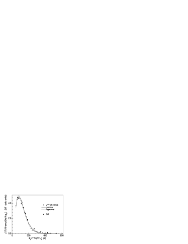
Figure 1: Anisotropy energy distributions obtained by the out-of-phase component of ac susceptibility ($\chi^{\prime\prime}/T$) and viscosity ($S/T$) measurements. Lognormal and gamma distribution fits to $\chi^{\prime\prime}/T$ data are shown.

Eq. II.1 can be further used to determine the proportionality between $E_{a}$ and $D^{3/2}$, $\alpha^{\prime}=18$ Knm^-3/2. As expected from the above equation, we observe that, in a $(E_{a}/\alpha^{\prime})^{2/3}$ scale, both distributions of $\chi^{\prime\prime}/T$ and $S/T$ superimpose to the diameter distribution (Fig. 2). This is a confirmation that describing $\chi/T$ and $S/T$ by a lognormal function is a good approximation for the identification of $p$ and $\alpha$.

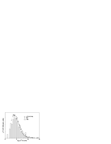
Figure 2: Diameter distribution determined by TEM compared to the anisotropy energy distributions obtained by $\chi^{\prime\prime}/T$ and $S/T$ in a $(E_{a}/\alpha^{\prime})^{2/3}$ scale, showing the scaling between $(E_{a}/\alpha^{\prime})^{2/3}$ and $D$. Using other powers $p^{\prime}$ such as 3, 2, or 1 gives unsatisfactory scaling.

Eq. 10 can be rewritten in terms of the particle volume as:

$$E_{a}=\alpha V^{1/2}$$ (11)

This means that the anisotropy barriers are randomly distributed in volume. In each particle, the effective value of $E_{a}$ is given by the fluctuation of local $E_{a}$. This requires that the local $E_{a}$ is a random homogeneous quantity. Such homogeneity is supported by the structure model, since it is composed of a single phase with in-volume defects, where we can expected $E_{a}$ to be locally different.

From Eq. 11 it is still possible to determine an effective anisotropy energy per volume, $K_{eff}$, that increases with decreasing $V$, following $V^{-1/2}$. In the 1 -10 nm $D$ range, $K_{eff}$ ranges from $4.7\times 10^{5}$ to $1.5\times 10^{4}$ J/m³, which are of the order of those found in the literature Gilles et al. (2000); Pankhurst and Pollard (1993). For the average size of the sample, $K_{eff}=2.9\times 10^{4}$ J/m³.

IV.2 Relationship between magnetic moment and size

Unlike the case of $E_{a}$, there is no direct measurement of the $\mu_{un}$ distribution. A way to obtain this distribution is to model the dependence of the magnetization with the field $M(H)$ to a given function of $\mu_{un}$ considering a $\mu_{un}$ distribution. A function usually applied to model $M(H)$ of nanoparticles is the Langevin function Makhlouf et al. (1997); Harris et al. (1999); Silva et al. (2005, 2006). This is a good approximation when surface effects and anisotropy are negligible. Anisotropy effects are expected to be relevant in AF nanoparticles due to coupling between $\mu_{un}$ and the AF axis Gilles et al. (2000); Madsen et al. (2006). In AF nanoparticles, anisotropy effects have been taken into account using a Néel (Ising-like) model, considering that $\mu_{un}$ can have only the AF axis direction Gilles et al. (2000). On the other hand, recent simulations show that $M(H)$ is greatly affected by surface effects, such that a one-spin approach as considered in the Langevin or Néel functions are crude approximations Kachkachi (2007).

Despite this situation, we have previously modelled $M(H)$ using a Langevin distributed function Silva et al. (2006) and found that the parameter $s$ of the $\mu_{un}$ lognormal distribution is $s_{\mu}=0.9$, so that $q=0.7\pm 0.1$ and $\mu_{un}\propto V^{2/3}$. We note that the value of $q$ here derived is different to that estimated in Ref. Silva et al. (2006) comparing the average values of the equivalent number of uncompensated ions and the total number of ions ($q=1/3$). Both $q$ values are obtained after the same fit procedure performed on the same $M(H)$ curves. The only difference is the approach for deriving $q$: using average values of the uncompensated moment and size or using the information about the distribution of both. This is an example of how the use of averages may lead to inaccurate estimations, since the pre-factor of the power law cannot be ignored. In this scenario the uncompensated moments were to lie on the particles surface, despite the fact that the energy barriers associated to the uncompensated moments are randomly distributed in volume.

At this point one should highlight that the Langevin distributed function may be a too crude description of $M(H)$ to yield a good estimation of $s_{\mu}$, so that a different scenario is possible: having no reliable estimation of $s_{\mu}$ we discuss the situation where the uncompensated moments are associated (proportional) to the energy barriers, so that a $\mu_{un}\propto V^{1/2}$, i. e. they are randomly distributed in volume. In fact, the uncompensated moments are those contributing to the Curie-like ac susceptibility and those experiencing the blocking phenomena associated with the onset of $\chi^{\prime\prime}$ and $S$. Therefore uncompensated moments should be those relevant in determining the relation between $E_{a}$ and $V$. Within this framework, $V^{1/2}$ may be regarded as the equivalent volume that contains the ferromagnetic-like uncompensated moments. Such relation between $\mu_{un}$ and $V^{1/2}$ was proposed for antiferromagnetic nanoparticles by Néel Néel (1961) and is consistent with magnetization measurements performed on ferritin Makhlouf et al. (1997); Harris et al. (1999); Silva et al. (2005).

V Conclusions

In this report we show that distributed samples can be used to investigate the relationship between the magnetic anisotropy barrier $E_{a}$ and the nanoparticles volume $V$ in a consistent manner. The relation is accessed by comparing the parameters of the lognormal distribution of both physical quantities. Size distribution was obtained by a TEM study and $E_{a}$ was obtained by two independent measurements: out-of-phase ac susceptibility and viscosity measurements. We have applied this method to a ferrihydrite nanoparticles system and found the relation between $E_{a}$ and $V$ in an antiferromagnetic material: $E_{a}\propto V^{1/2}$. This shows that the magnetic anisotropy barriers are randomly distributed in the volume, in accordance to recent structure studies.