Fano-Kondo effect in a two-level system with triple quantum dots: shot noise characteristics

Abstract

We theoretically compare transport properties of Fano-Kondo effect with those of Fano effect. We focus on shot noise characteristics of a triple quantum dot (QD) system in the Fano-Kondo region at zero temperature, and discuss the effect of strong electric correlation in QDs. We found that the modulation of the Fano dip is strongly affected by the on-site Coulomb interaction in QDs.

Quantum dot (QD) systems have attracted a lot of interest over many years because of their variety of controllability of small number of electrons in order to understand many-body effects in electronic systems. Quantum correlation between localized states in QDs and free electrons in electrodes induces interesting phenomena such as the Fano effect and the Kondo effect. A number of important experiments have been carried outFano ; Tarucha ; Gores ; Sato ; Kobayashi ; Otsuka ; Rushforth ; Sasaki and many theories have been proposedKang ; Aligia ; Wu ; triple ; TanaNishi . The Fano effect occurs as a result of quantum interference between a discrete energy state and a continuum stateFano . The Kondo effect is observed as a result of many-body correlations where internal spin degrees of freedom play an important roleTarucha . The Fano-Kondo effect, which is a combination of the Fano effect and the Kondo effect, can be observed when on-site Coulomb interaction in a QD is strongSato . A T-shaped QD is considered to be suitable for discussing the Fano-Kondo effectSato ; Kobayashi ; Otsuka ; Kang ; Aligia ; Wu .

Quantum and thermal fluctuations are main obstacles for observing quantum correlations, and are estimated through current noise characteristics. Shot noise is a zero frequency limit of noise power spectrum and provides various information on correlation of electrons. For uncorrelated electrons, shot noise $S_{I}$ shows Schottky result $S_{I}=2eI$ where $e$ is an electronic charge and $I$ is an electric current. The ratio of shot noise $S_{I}$ and full Poisson noise $2eI$ ($I$ is an average current), $\gamma\equiv S_{I}/(2eI)$, is called the Fano factor, and indicates important noise properties.

We have theoretically investigated transport properties of the triple QD system depicted in Fig.1, where QDs $a$ and $b$ are connected to electrodes through QD $d$TanaNishi . This triple-QD system is considered to be in the same category as the T-shaped QD. When coupling between QD $a$ and $b$ is larger than that between QD $b$ and $d$ ($t_{C}>t_{d}$), we can use this setup as apparatus for detecting two-level system (QD $a$ and QD $b$) by a QD $d$ with electrodes (Hereafter we call QD $d$ a detector QD). Moreover, when the number of electrons is controlled, double QD $a$ and $b$ can be regarded as a charge qubittana0 ; Gilad with a Fano interference detector QD. In Ref.TanaNishi , we have shown that the Fano dip is modulated for a slow detector with no on-site Coulomb interaction in QD $d$. However, noise properties, which are considered to be related to decoherence, has not been clarified. Although $1/f$ noise induced by undesired trap sites is shown to be the largest cause of decoherenceAstafiev , shot noise is also a measure of decoherence in solid-state systems.

Wu et al.Wu calculated noise properties of T-shaped QD system and showed that shot noise strongly depends on the coupling strength between a side QD and a detector QD. As tunneling coupling between side QD and detector QD increases, $\gamma$ quickly increase up to the Poisson value ($\gamma=1$). López et al. calculated shot noise of serially and laterally coupled double QD system and showed that $\gamma$ strongly depends on the coupling strength between QDsLopez . Thus, $\gamma$ and shot noise reflect the coupling configuration of QD system and provide important information about the electronic structure of the system.

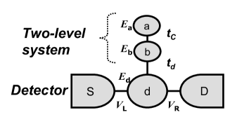
Figure 1: Schematic plot of triple QD system. QDs $a$ and $b$ constitute a two-level system that is coupled to QD $d$ only which is connected to the electrodes.

Here, we compare zero temperature shot noise properties of the Fano-Kondo effect with those of the Fano effect, in order to reveal the effect of strong on-site Coulomb interaction on the transport properties. The former case has stronger constraint than the latter case. We assume an infinite Coulomb interaction for QD $a$ and $b$ and no Coulomb interaction for QD $d$ ($U_{a}=U_{b}=\infty$, $U_{d}=0$) for the Fano-Kondo case. For the Fano case, we consider that there is no on-site Coulomb interaction for all QDs ($U_{a}=U_{b}=U_{d}=0$). This corresponds to a case in which there is one degree of freedom Otsuka ; Mahan such that QDs are large without a spin scattering. For simplicity, we assume that there is a single energy level in each QD and that the two energy levels of QD $a$ and QD $b$ coincide and correspond to gate voltages that are applied to those QDs. We use slave-boson mean-field theory (SBMFT) based on the nonequilibrium Keldysh Green’s function method. The formulation of SBMFT is very useful and a good starting point for studying the transport properties of a strongly correlated QD system, although this method is usable at a lower temperature ($T$) region than the Kondo temperature $T_{K}$Newns ; Lopez .

Formulation—. Hamiltonian is constructed from electrode parts, QD parts, tunneling parts between an electrode and a QD, and those between QDs. For the Fano-Kondo case, additional constraint is required. The mean-field Hamiltonian for the Fano-Kondo case is described in terms of slave-bosons $b_{\alpha_{1}}$ $(\alpha_{1}=a,b)$ as:

$$H^{\rm FK}=\sum_{\alpha=L,R}\sum_{k_{\alpha},s}E_{k_{\alpha}}c_{k_{\alpha}s}^{\dagger}c_{k_{\alpha}s}+\sum_{\alpha_{1}=a,b,d}\sum_{s}E_{\alpha_{1}}f_{\alpha_{1}s}^{\dagger}f_{\alpha_{1}s}+\sum_{\alpha_{1}=a,b}\lambda_{\alpha_{1}}\left(\sum_{s}f_{\alpha_{1}s}^{\dagger}f_{\alpha_{1}s}+b_{\alpha_{1}}^{\dagger}b_{\alpha_{1}}-1\right)$$ (1)

$$+ \!\frac{t_{C}}{N}\sum_{s}(f_{as}^{\dagger}b_{a}b_{b}^{\dagger}f_{bs}+f_{bs}^{\dagger}b_{b}b_{a}^{\dagger}f_{as})+\frac{t_{d}}{N}\sum_{s}(f_{ds}^{\dagger}b_{b}^{\dagger}f_{bs}+f_{bs}^{\dagger}b_{b}f_{ds})+\sum_{\alpha=L,R}\frac{V_{\alpha}}{\sqrt{N}}\sum_{k_{\alpha},s}(c_{k_{\alpha}s}^{\dagger}f_{ds}+f_{ds}^{\dagger}c_{k_{\alpha}s})$$

where $E_{k_{\alpha}}$ is the energy level for source ($\alpha=L$) and drain ($\alpha=R$) electrodes. $E_{a}$, $E_{b}$ and $E_{d}$ are energy levels for the three QDs, respectively. $t_{C}$, $t_{d}$ and $V_{\alpha}$ are the tunneling coupling strength between QD $a$ and QD $b$, that between QD $b$ and QD $d$, and that between QD $d$ and electrodes, respectively. $c_{k_{\alpha}s}$ and $f_{\alpha_{1}s}$ are annihilation operators of the electrodes, and of the three QDs $(\alpha_{1}=a,b,d)$, respectively. $s$ is spin degree of freedom with spin degeneracy $N$; here we apply $N=2$. $\lambda_{\alpha_{1}}$ is a Lagrange multiplier. We take $z_{\alpha_{1}}\equiv b_{\alpha_{1}}^{\dagger}b_{\alpha_{1}}/2$ and $\tilde{E}_{\alpha_{1}}\equiv E_{\alpha_{1}}+\lambda_{\alpha_{1}}$ as mean-field parameters for QD $a$ and QD $b$. The Hamiltonian for the Fano case is similar to $H^{\rm FK}$ except that $\lambda_{a}=\lambda_{b}=0$ and $b_{a}=b_{b}=1$ in Eq.(1).

In the Fano-Kondo effect, four self-consistent equations to determine mean-field parameters $\lambda_{\alpha_{1}}$ and $b_{\alpha_{1}}$ ($\alpha_{1}=a,b$) are required and expressed as

$$\tilde{t}_{C}\sum_{s}\langle f_{bs}^{\dagger}f_{as}\rangle\!+\!\lambda_{a}|b_{a}|^{2}=0,$$ (2)

$$\tilde{t}_{C}\sum_{s}\langle f_{as}^{\dagger}f_{bs}\rangle+\tilde{t}_{d}\sum_{s}\langle f_{ds}^{\dagger}f_{bs}\rangle\!+\!\lambda_{b}|b_{b}|^{2}=0,$$ (3)

$$\sum_{s}\langle f_{\alpha_{1}s}^{\dagger}f_{\alpha_{1}s}\rangle+|b_{\alpha_{1}}|^{2}=1,\ \ (\alpha_{1}=a,b),$$ (4)

Current and noise formula are expressed by Keldysh Green’s functions. Keldysh Green’s functions are obtained by applying analytic continuation rules to the equations of motion, which are derived from the above HamiltonianNewns ; Lopez . For example, Green’s functions for QDs are given as $G_{aa}^{r}(\omega)=[(\omega-\tilde{E}_{b})B_{r}-|\tilde{t}_{d}|^{2}]/B_{00}$, $G_{bb}^{r}(\omega)=[(\omega-\tilde{E}_{a})B_{r}/B_{00}$ and $G_{dd}^{r}(\omega)=D_{ab}/B_{00}$ etc., where $D_{ab}\equiv(\omega-\tilde{E}_{a})(\omega-\tilde{E}_{b})-\tilde{t}_{c}^{2}$, $B_{r}\equiv\omega-\tilde{E}_{d}+i\Gamma$ and $B_{00}\equiv{D_{ab}B_{r}-(\omega-\tilde{E}_{a})|\tilde{t}_{d}|^{2}}$ with $\tilde{t}_{C}=t_{C}b_{a}b_{b}^{\dagger}/N$ and $\tilde{t}_{d}=t_{d}b_{b}^{\dagger}/N$. Here, $\Gamma_{\alpha}\equiv 2\pi\rho_{\alpha}(\mu_{\alpha})|V_{\alpha}|^{2}$ is the tunneling rate between $\alpha$ electrode and QD $d$ with a density of states (DOS), $\rho_{\alpha}(\mu_{\alpha})$, for each electrode at Fermi energy $\mu_{\alpha}$. $\Gamma\equiv(\Gamma_{L}+\Gamma_{R})/2$ and we assume $\Gamma_{L}=\Gamma_{R}$.

Source current $I_{L}$ is expressed as

$$I_{L}=\frac{2e}{h}\int_{-\infty}^{\infty}d\omega T(\omega)(f_{L}(\omega)-f_{R}(\omega))$$ (5)

where transmission probability $T(\omega)$ is given as

$$T(\omega)=\frac{\Gamma_{L}\Gamma_{R}|D_{ab}|^{2}}{[D_{ab}(\omega-E_{d})-(\omega-\tilde{E}_{a})z_{a}t_{d}^{2}/2]^{2}+\Gamma^{2}D_{ab}^{2}/4}$$ (6)

(the denominator is $B_{00}$) and Fermi distribution functions $f_{\alpha}(\omega)\equiv[\exp((\omega-\mu_{\alpha})/T)+1]^{-1}$ where we set symmetrical bias condition: $\mu_{L}=E_{F}-eV/2$ and $\mu_{R}=E_{F}+eV/2$ with $E_{F}=0$. Note that in the present case we can check that $I_{L}$ and $I_{R}$ are symmetric and satisfy a current conservation. Conductance is given as $G=-\frac{2e}{h}\int d\omega T(\omega)\frac{\partial f_{L}(\omega)}{\partial\omega}$. The transmission probability is related to a DOS of the detector QD $\rho_{d}(\omega)=-{\rm Im}G_{dd}^{r}(\omega)/\pi$ such as $T(\omega)=\frac{2\Gamma_{L}\Gamma_{R}}{\Gamma_{L}+\Gamma_{R}}\pi\rho_{d}(\omega),$ which means that we can discuss characteristics of DOS similar to a transmission probability.

Current noise is calculated as a correlation function of current fluctuation as $S(t,t^{\prime})=\frac{1}{2}$ $[\langle\{\hat{I}_{L}(t),\hat{I}_{L}(t^{\prime})\}\rangle-2\langle\hat{I}_{L}(t)\rangle^{2}],$ where $\hat{I}_{L}(t)=(ie/\hbar)\sum(V_{L}/\sqrt{N})[c_{k_{L}s}^{\dagger}(t)f_{ds}(t)-\mbox{H.c.}]$ is a current operator. A derivation procedure similar to that in Ref.Lopez is applied to our case, we obtained noise formula at $T=0$ as

$$S(V)=\frac{4e^{2}}{h}\int_{-eV/2}^{eV/2}d\omega T(\omega)(1-T(\omega)).$$ (7)

The Fano factor $\gamma$ at zero bias $V=0$ is obtained by $\gamma=1-T(E_{F})$, and indicates that shot noise is in the sub-Poissonian region ($\gamma<1$). Similar to Ref.TanaNishi , we classify our triple QD system by magnitude of $t_{C}/t_{d}$ and $\Gamma/t_{d}$. The ratio $t_{C}/t_{d}$ compares the internal coupling strength in a two-level system with that between the two-level system and the detector, and we regard the case where $t_{C}/t_{d}=5$ as a strongly coupled two-level system and the case where $t_{C}/t_{d}=1$ as a weakly coupled two-level system. If $\Gamma/t_{d}$ is large, the electron that flows through QD $d$ is so fast that it cannot detect the oscillation of an electron in the coupled QDs $a$ and $b$. If $\Gamma/t_{d}$ is small, the electron that flows through QD $d$ can observe the evidence of bonding and antibonding states. We call a detector with large $\Gamma/t_{d}=2$ a fast detector, and one with smaller $\Gamma/t_{d}=0.4$ a slow detector. We assume that $D=20t_{d}$, $|E_{d}|<0.4t_{d}$, $\Gamma>0.4t_{d}$ and $E_{F}=0$ ($D$ is a bandwidth). Then, we have $T_{K}\sim De^{-\pi|\tilde{E}_{d}-E_{F}|/\Gamma}$ $\sim 1.6t_{d}$.

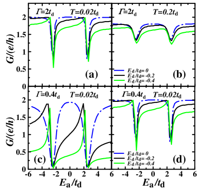
Figure 2: Conductance $G$ as a function of an energy level of the two-level system $E_{a}(=E_{b})$ with a strong coupling ($t_{C}/t_{d}=5$) for the Fano case ($U_{a}=U_{b}=0$). (a) $T/t_{d}=0.02$ and (b) $T/t_{d}=0.2$ for a fast detector ($\Gamma/t_{d}=2$). (c) $T/t_{d}=0.02$ and (d)$T/t_{d}=0.2$ for a slow detector ($\Gamma/t_{d}=0.4$). $E_{F}=0$.

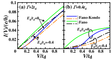
Figure 3: $I$-$V$ characteristics for a strong coupling ($t_{C}/t_{d}=5$) at $T=0$. (a) Fast detector ($\Gamma/t_{d}=2$) and (b) slow detector ($\Gamma/t_{d}=0.4$). $E_{a}=E_{b}=0=E_{F}$.

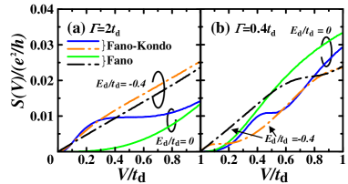
Figure 4: Shot noise as a function of bias voltage for a strong coupling ($t_{C}/t_{d}=5$). (a) Fast detector($\Gamma/t_{d}=2$). (b) Slow detector($\Gamma/t_{d}=0.4$). $T=0$. $E_{a}=E_{b}=0=E_{F}$.

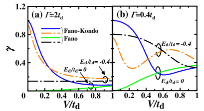
Figure 5: Fano factor $\gamma$ as a function of bias voltage. $E_{a}=E_{b}=0=E_{F}$ for a strong coupling ($t_{C}/t_{d}=5$). (a) Fast detector($\Gamma/t_{d}=2$) and (b) slow detector($\Gamma/t_{d}=0.4$).

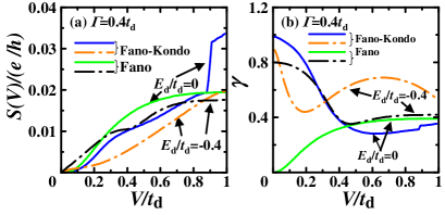
Figure 6: Weak coupling case($t_{C}/t_{d}=1$) for a slow detector ($\Gamma/t_{d}=0.4$). (a) Shot noise and (b) Fano factor $\gamma$ as a function of bias voltage. $T=0$. $E_{a}=E_{b}=0=E_{F}$.

Numerical calculations.— Here, we show numerical results of our triple QD system in the Fano-Kondo effect and the Fano effect. First, Fig. 2 shows conductance of the Fano case as a function of $E_{a}$. We can see a clear double-peak structure in every figure. This is in a large contrast with our previous results of the Fano-Kondo effects(Ref.TanaNishi ) where modulation of a single Fano dip can be seen only by a slow detector ($\Gamma=0.4t_{d}$) at low temperature ($T=0.02t_{d}$). The present clear double-peak structure is a direct result of the form of transmission probability $T(\omega)$, in particular, $D_{ab}$ in the numerator of Eq.(6). These results show that Kondo effect, spin exchange effect, greatly changes the Fano effect. Dip structure is the largest for a slow detector at low temperature (Fig.2(c)). The asymmetry of the dip structure for $E_{d}\neq 0$ can also be understood from Eq.(6). Because $G\propto T(\omega\sim 0)$ at low temperature and we set $E_{a}=E_{b}$, we have $D_{ab}(\omega=0)=\tilde{E}_{a}^{2}-\tilde{t}_{c}^{2}$. Thus, for $E_{d}=0$, both the numerator and the denominator of $T(\omega)$ are symmetric for $E_{a}$. However, when $E_{d}\neq 0$, the denominator deviates from symmetric form because of the $D_{ab}(\omega-E_{d})$ in the expression.

Figure 3 shows current-voltage ($I$-$V$) characteristics at $T=0$. We can see that all current looks similar for a fast detector ((a)) for both the Fano effect and the Fano-Kondo effect. This indicates that a fast detector is less sensitive to quantum states of QD system than a slow detector. Current of the Fano-Kondo effect is always less than that of the Fano effect. This indicates that stronger electronic correlation in QD $d$ suppresses its current.

Figure 4 shows shot noise characteristics as a function of bias voltage across the detector QD. $E_{d}$ dependence is simpler for a fast detector ((a)). This is because a fast detector is more sensitive to energy level of a detector QD $d$ than energy levels in two-level system. Shot noise of a slow detector reflects internal states of two-level system.

Although magnitude of current for a fast detector is larger than that for a slow detector (Fig. 3), magnitude of shot noise for a fast detector is of the same order as that of a slow detector (Fig. 4). Thus, $\gamma$ for a slow detector is relatively larger than that for a fast detector as shown in Fig. 5. This is because of the stronger coupling of flowing electrons with two-level states in a slow detector. Strong nonlinearity can be seen around $V=0$, because energy levels of QDs are close to a Fermi energy ($E_{a}=E_{b}=0=E_{F}$) and strongly coupled with electrode electrons. In both a fast detector and a slow detector, $\gamma$ for the Fano-Kondo case is larger than that for the Fano case. This indicates that stronger electronic correlation induces more noise.

Figures 6(a) and (b) show shot noise and $\gamma$ of weak coupling ($t_{C}/t_{d}=1$) for a slow detector ($\Gamma/t_{d}=0.4$). Similar to Fig. 4 (b), shot noise is modulated by changing $E_{d}$ reflecting a two-level state. Compared with Fig.4, Fig. 6(a) shows that modulation by $E_{d}$ becomes more complicated. This is because energy levels of weakly coupled triple QDs are more close with each other than those of strongly coupled QDs. Figure 6 (b) shows $\gamma$ characteristics for a weakly coupled slow detector. We can see that values of $\gamma$ become closer with each other, reflecting closer coupling between QDs.

Discussion.— Our numerical results show that, as coupling in a two-level state (qubit) becomes stronger, noise increases. In addition, a slower detector, which is found to be more desirable for reading out a two-level state, induces more noise than a fast detector. Thus, there is a trade-off in that reading out more detailed information induces more noise or larger Fano factor. Appropriate parameters ($t_{C}/t_{d}$, $\Gamma/t_{d}$ etc.) should be determined depending on sensitivity of the external circuit connected to this triple QD system. As noted in the introduction, in order to use the two-level state as a qubit, a stronger constraint is required so that one excess electron stays in the two-level system. This would be realizable, for example, by forming smaller and closely coupled QDs, such that two electrons are not permitted into the QDs because of their repulsive Coulomb interaction. As shown in the numerical results, the Fano factor for stronger correlation (Fano-Kondo case) is larger than that for weaker correlation (Fano case). Thus, it is possible that we will have to accept larger back-action when introducing charge qubit condition. More elaborate control of the measurement setup would be required for a charge qubit system.

Kobayashi et al.Kobayashi discussed the rapid smearing out of the dip structure with increasing temperature mainly owing to thermal broadening. Although we assume one energy level in each QD at $T=0$, if we take more energy levels in each QD into consideration, the Fano dip would smear out rapidly with increasing temperature.

In conclusion, focusing on the Fano effect and the Fano-Kondo effect in a two-level state, we studied noise properties of a triple QD system. We have shown that, depending on the coupling strength among the triple QDs, noise and the Fano factor are greatly modulated for a slow detector. In particular, we found that detailed reading of a two-level state is inclined to increase noise characteristics of the system.

We are grateful to A. Nishiyama, J. Koga, R. Ohba, T. Otsuka and M. Eto for valuable discussions.

References

- (1) U. Fano Phys. Rev. 124, 1866 (1961).
- (2) W. G. van der Wiel et al., Science 289 2105 (2000).
- (3) J. Göres et al., Phys. Rev. B62, 2188 (2000).
- (4) M. Sato et al.,Phys. Rev. Lett. 95, 066801 (2005).
- (5) K. Kobayashi et al., Phys. Rev. 70, 035319 (2004).
- (6) T. Otsuka et al.,J. Phys. Soc. Jpn. 76 084706 (2007).
- (7) A. W. Rushforth et al., Phys. Rev. B 73, 081305(R) (2006).
- (8) S. Sasaki et al., Phys. Rev. B 73, 161303(R) (2006).
- (9) K. Kang et al., Phys. Rev. B 63, 113304 (2001).
- (10) A. A. Aligia and C. R. Proetto, Phys. Rev. B 65, 165305 (2002).
- (11) B. H. Wu et al.,Phys. Rev. B72, 165313 (2005).
- (12) C. A. Büsser et al., Phys. Rev. 70, 035402 (2004); Z.-T. Jiang et al., Phys. Rev. B72, 045332 (2005).
- (13) T. Tanamoto and Y. Nishi, arXiv:0704.3863, to be published in Phys. Rev. B.
- (14) T. Tanamoto and X. Hu, Phys. Rev. B69, 115301 (2004).
- (15) T. Gilad and S.A. Gurvitz, Phys. Rev. Lett. 97, 116806 (2006); H. S. Goan et al., Phys. Rev. B 63, 125326 (2001).
- (16) O. Astafiev et al.,Phys. Rev. Lett. 96, 137001 (2006).
- (17) R. López et al., Phys. Rev. B 69, 235305 (2004).
- (18) G. D. Mahan, ”Many-Particle Physics”, Plenum Press, New York and London, 1981.
- (19) D M. Newns and N. Read, Adv. Phys. 36, 799 (1987).