XMM-Newton, Chandra, and CGPS observations of the Supernova Remnants G85.4+0.7 and G85.9$-$0.6

Abstract

We present an XMM-Newton detection of two low radio surface brightness SNRs, G85.4+0.7 and G85.9$-$0.6, discovered with the Canadian Galactic Plane Survey (CGPS). High-resolution XMM-Newton images revealing the morphology of the diffuse emission, as well as discrete point sources, are presented and correlated with radio and Chandra images. The new data also permit a spectroscopic analysis of the diffuse emission regions, and a spectroscopic and timing analysis of the point sources. Distances have been determined from H I and CO data to be $3.5\pm 1.0$ kpc for SNR G85.4+0.7 and $4.8\pm 1.6$ kpc for SNR G85.9$-$0.6.

The SNR G85.4+0.7 is found to have a temperature of $\sim 12-13$ MK and a 0.5–2.5 keV luminosity of $\sim 1-4\times 10^{33}D^{2}_{3.5}$ erg/s (where $D_{3.5}$ is the distance in units of 3.5 kpc), with an electron density $n_{e}$ of $\sim 0.07-0.16(fD_{3.5})^{-1/2}$ cm^-3 (where $f$ is the volume filling factor), and a shock age of $\sim 9-49(fD_{3.5})^{1/2}$ kyr.

The SNR G85.9$-$0.6 is found to have a temperature of $\sim 15-19$ MK and a 0.5–2.5 keV luminosity of $\sim 1-4\times 10^{34}D^{2}_{4.8}$ erg/s (where $D_{4.8}$ is the distance in units of 4.8 kpc), with an electron density $n_{e}$ of $\sim 0.04-0.10(fD_{4.8})^{-1/2}$ cm^-3 and a shock age of $\sim 12-42(fD_{4.8})^{1/2}$ kyr.

Based on the data presented here, none of the point sources appears to be the neutron star associated with either SNR.

1. Introduction

In 2001, two new supernova remnants (SNRs) with low radio surface brightness, G85.4+0.7 and G85.9$-$0.6, were discovered in Canadian Galactic Plane Survey (CGPS)(Taylor et al., 2003) data and confirmed in X-rays with ROSAT data (Kothes et al., 2001). Both show distinct shells in the radio band with an extended region of X-ray emission in the centre. The radio surface brightness of G85.4+0.7 at 1 GHz is $\Sigma_{1{\rm GHz}}\leq 1\times 10^{-22}$ Watt ${\rm m}^{-2}$ ${\rm Hz}^{-1}$ ${\rm sr}^{-1}$ and the radio data also indicate that the SNR has a non-thermal shell with angular diameter $\approx 0.4^{\circ}$ which is surrounded by a thermal shell with an angular diameter of $\approx 0.6^{\circ}$ and is located within an H I bubble. The bubble also contains two B stars which may have been part of the same association as the SNR’s progenitor star. G85.9$-$0.6 has a radio surface brightness $\Sigma_{1{\rm GHz}}\leq 2\times 10^{-22}$ Watt ${\rm m}^{-2}$ ${\rm Hz}^{-1}$ ${\rm sr}^{-1}$ and it has no discernible H I features, indicating that it is expanding into a low density medium, perhaps between the local and Perseus spiral arms. The most likely event which would produce an SNR in such a region would be a Type Ia supernova.

X-ray observations are important to the study of SNRs, particularly those with low surface brightness, because they provide information about the morphology and emission processes of these objects, which are indicators of both the nature of the supernova explosion which formed them and the properties of the progenitor star. SNRs with low surface brightness are expected to be formed after the core collapse of a massive star in a Type Ib/c or Type II explosion, because the stellar wind would have blown away much of the interstellar medium (ISM) surrounding it, leaving a low ambient density into which the shock from the supernova expands. A Type Ia supernova can also result in a low surface brightness SNR if the surrounding ISM has a low density, such as it would if it were located between two spiral arms of the galaxy. Thermal X-ray emission from a SNR arises as the blast wave of the explosion travels through and shocks the ISM, and as a reverse shock travels back into and shocks the ejecta. The X-ray spectrum of the SNR gives information about the temperature, the density, and the luminosity of the shocked material, while imaging data provides information about the size and morphology of the region.

The low angular and spectral resolutions as well as the small number of counts in the ROSAT data did not allow spectroscopy nor detailed imaging to be done, so XMM-Newton observations, described in §2, have been made in order to confirm the detection of the SNRs, and to perform imaging, spectroscopic and timing studies. Detailed X-ray imaging, described in §3, is used to map the diffuse emission and compare it to the location and size of the radio shells, and Chandra data have been used to search for compact objects not resolved by XMM. Spectral parameters obtained in §4 lead to an estimate of such quantities as temperature, density, and luminosity of the SNRs. In §5 the point sources are catalogued and an attempt at identification is made by matching their positions to objects in other catalogues. Timing analysis is performed to identify any pulsar candidates. The distances to the SNRs are derived from H I and CO data in §6. The results are discussed in §7.

Preliminary results were presented in Jackson, Safi-Harb, & Kothes (2006) and Safi-Harb (2006).

2. Observations

2.1. XMM-Newton Observations

SNR G85.4+0.7 was observed with XMM-Newton on 2005 May 31 for 11.5 ks (Obs ID: 0307130101, PI: S. Safi-Harb) and again on October 27 for 15.2 ks (Obs ID 0307130301, PI: S. Safi-Harb), because of proton flares in the first observation which made a large fraction of the data unusable. A 29 ks XMM-Newton observation was made of SNR G85.9$-$0.6 on 2005 November 24 (Obs ID 0307130201, PI: S. Safi-Harb).

The PN (Strüder et al., 2001) and MOS (Turner et al., 2001) data were reduced with the latest version of SAS (6.5.0) and events during proton flares were filtered out for producing images and spectra by using the SAS routines evselect to create rate files and tabgtigen to generate good time intervals (GTIs) for filtering the event files with the evselect routine. This rendered the first observation of G85.4+0.7 useful only for imaging, and slightly reduced the integration time, from 29 ks to 26 ks for the G85.9$-$0.6 observation. The second observation of G85.4+0.7 shows no evidence for proton flaring and the removal of proton flares did not significantly reduce the integration time. Images and spectra were created from the event files using evselect. The total effective exposure time for G85.4+0.7 was 14 ks for PN and 16 ks for the MOS instruments and for G85.9$-$0.6 it was 23 ks for PN and 26 ks for MOS.

To facilitate source detection, exposure maps were made using eexpmap and the images were combined using emosaic. The spectra were binned using a minimum of 25-50 counts per bin for the MOS instruments and 50 or 100 counts per bin for the PN for the point source and diffuse spectra respectively, using grppha. This latter grouping was necessary because the background subtraction added excessive noise to the spectra, particularly at high energies, where the spectra are background-dominated. The background for both SNRs was calculated using various methods described in §4.1.

2.2. Chandra Observations

A 14.5 ks observation of SNR G85.4+0.7 was made on 2003 January 26 (Obs ID: 3898, PI: S. Safi-Harb) by the Advanced CCD Imaging Spectrometer (ACIS-S; G. Garmire). SNR G85.9$-$0.6 was observed with ACIS-S for 20.2 ks on 2003 October 3 (Obs ID: 3899, PI: S. Safi-Harb). Both observations were made at a focal plane temperature of $-120^{\circ}$C.

The analysis of the Chandra data was done using Chandra Interactive Analysis of Observations (CIAO version 3.3). For both Chandra observations, the data were corrected for charge transfer inefficiency (CTI) with tools provided by the ACIS team of Pennsylvania (Townsley et al., 2000). Events with ASCA grades (0, 2, 3, 4, 6) were retained, and periods of high background rates were removed. Data from hot pixels were eliminated. The effective exposure time for the observation of SNR G85.4+0.7 was 14.3 ks and for SNR G85.9$-$0.6 it was 19.9 ks. The backgrounds for the point source spectra were extracted from annuli surrounding the sources. The spectra were grouped with a mimimum of 30 counts in each bin. Data from the S2 and S3 chips were used. Data from the other chips were not used because they do not overlap the XMM field of view.

3. Imaging

The previous X-ray images from the ROSAT All-Sky Survey did not resolve the SNRs and the point sources in the field, so the XMM-Newton PN and MOS data can be used to determine the nature of the sources. The results are described below.

3.1. G85.4+0.7

The 0.5–2.5 keV XMM-Newton PN and MOS mosaic image of G85.4+0.7 with radio contours overlaid is shown in Figure 1. The image includes only energies between 0.5 and 2.5 keV in order to match the ROSAT bandpass and because there is negligible diffuse emission above 2.5 keV. The X-ray image is smoothed with a Gaussian filter with a 3 pixel radius. The X-ray emission is in the same location and is a similar angular size as indicated by the ROSAT data, shown in Figure 6 of Kothes et al. (2001), with an approximate angular radius of 6.7^′. It is much better resolved, however, and the regions of diffuse emission and the point sources are clearly visible.

The top two panels of Figure 2 show the 0.5–2.5 keV and 2.5–10 keV XMM-Newton images of G85.4-0.7, smoothed in the same way as Figure 1. The absence of diffuse emission in the hard X-ray band is clear from the middle panel. The lower panel shows the 0.5–2.5 keV image with sources subtracted, smoothed further and scaled to emphasize the diffuse emission, and smoothed contours are overlaid to show the morphology of the remnant. The contours indicate a centrally filled morphology with a slightly elongated shape. The circles in the top panel indicate spectral extraction regions described in §4.2 and §7.3.

There are nine point sources in the image from which spectra can be extracted, and the analysis is described in §5. The extraction regions for the spectra, including the background for the diffuse emission, are indicated and labeled in Figure 2, and the spectral analysis of the diffuse emission is described in §4.2.

The Chandra image of SNR G85.4+0.7 is shown in Figure 3. The extraction regions used for the source and background regions are shown, and the applicable regions from the XMM-Newton observation are overlaid. The wavdetect tool in CIAO is used for source detection. Six of the point sources identified with XMM-Newton (1, 2, 3, 4, 6 and 7) are clearly visible on the Chandra image. Twelve additional sources appear on the Chandra image (labeled 10$-$21) but the spectra extracted from these point sources do not contain enough counts to enable meaningful spectral analysis, so while they are potential neutron star candidates and sources 10, 11, 12, 13, 15, and 16 are situated well within the radio shell of the SNR, further investigation of these sources is not possible at this time.

3.2. G85.9$-$0.6

The XMM-Newton PN and MOS mosaic image of G85.9$-$0.6 with radio contours overlaid is shown in Figure 4. The image is smoothed in the same way as the G85.4+0.7 image, with a Gaussian filter with a three-pixel radius. As with G85.4+0.7, the angular radius of approximately 5.8^′ and location of the X-ray emission shown in this figure matches that of Figure 6 of Kothes et al. (2001) and many features are resolved. 0.5–2.5 keV and 2.5–10.0 keV X-ray images are shown in the top two panels of Figure 5. It is clear from the hard X-ray image that the SNR does not appear above 2.5 keV, and the X-ray spectrum is background dominated above 2.5 keV, as will be explored in §4.3. The bottom panel of Figure 5 shows the same data as in the top panel with point source emission subtracted, scaled to emphasize the diffuse emission. The contours in the bottom panel are smoothed to show the overall morphology of the remnant. The diffuse X-ray emitting region seems to be round in shape, indicating a centrally filled X-ray morphology. The circles in the top panel indicate spectral extraction regions described in §4.3 and §7.4.

Spectra were extracted from 8 point sources and the diffuse region, as indicated in the top panel of Figure 5. The analysis of the spectrum from the diffuse region is described in §4.3, and §5 describes the analysis of the point sources.

Figure 6 shows the Chandra image of SNR G85.9$-$0.6. The locations of the extraction circles for sources 1 and 8 in the XMM-Newton image are shown, in addition to the additional point sources found on the Chandra image (labeled 9$-$27). The Chandra image does not show any point sources which have sufficient counts to do independent spectroscopic analysis, and only one of the sources identified from the XMM-Newton image (source 8) lies within the field of view of the Chandra image, with which a Chandra source has been identified.

4. Spectroscopy

The spectra from the regions of diffuse emission were extracted from areas indicated in Figures 2 and 5 for both PN and MOS. The diffuse emission regions and point sources are indicated and labeled in the Figures.

The spectra of the diffuse emission for both SNRs were fit to various models: a simple bresstrahlung model with gaussian lines, VMEKAL, VNEI, and VPSHOCK, each modified by interstellar absorption, in this case the Wisconsin absorption model (wabs in XSPEC, Morrison & McCammon (1983)). VMEKAL is a collisional ionization equilibrium model based on the model calculations of Mewe et al. (1985) of the emission spectrum from hot diffuse gas with Fe calculations by Liedahl et al. (1990), with variable abundances. VPSHOCK is a non-equilibrium ionization (NEI) model with variable abundances which models a plane parallel shock in a plasma with constant electron temperature T and a range of ionization timescales with an upper limit $\tau=n_{e}t$, where $n_{e}$ is the postshock electron density and $t$ is the shock age (Borkowski et al., 2001). VNEI is a NEI model similar to VPSHOCK, except with a single ionization timescale.

4.1. Background Estimation

Spectra of diffuse faint regions require particular attention to be paid to the choice of background region. Instrumental emission lines can dominate the spectrum if the background region is poorly chosen, leading to errors in spectral fits and a discrepancy between the PN and MOS spectra. The intuitive background region would be a relatively source free one at approximately the same galactic latitude as the source to minimize contamination by the Galactic ridge. However, because the effect of instrumental emission lines is not uniform with position on the CCDs, particularly on the PN instrument (Lumb, 2002), and exceeds the variation with galactic latitude for these observations, the background regions were chosen as closely as possible to the point opposite the source region through the centre of the image, taking care that there is no overlap between the source and background regions and omitting regions around point sources. The background regions for both SNRs are necessarily smaller than the source regions, but very little change in the spectral fits resulted from choosing various background regions in the same general area of the image.

An attempt has been made to estimate the MOS background spectra using the XMM-Newton Extended Source Analysis Software (XMM-ESAS) (Snowden & Kuntz, 2006). As yet, background estimation for the PN instrument is not included in this package. Data from filter wheel closed observations and from the unexposed corners of the MOS CCDs are used to generate background spectra. This serves as a test of the backgrounds generated from the observation itself, described above. To fit spectra using the XMM-ESAS backgrounds, it is necessary to include some additional spectral components, as recommended in Snowden & Kuntz (2006). Unabsorbed Gaussian lines of zero width at energies of 1.49 and 1.75 keV are fit to the MOS spectra in addition to the model describing the emission from the SNR. The 1.75 keV line was also added to the fit to the MOS spectra using the observation background. It was not necessary to add the 1.49 keV line to the fit of the G85.4+0.7 MOS spectra using observation backgrounds because it was adequately subtracted, but the 1.49 keV line was added to the G85.9$-$0.6 MOS spectra using observation backgrounds. It was also necessary to include a low energy broken power law component to the G85.9$-$0.6 fit of the ESAS-subtracted spectrum, as instructed in the ESAS documentation, to correct for instrumental effects, because the statistics allowed residuals at low energies to be clearly seen in the ESAS background subtracted spectra. The broken power law was not added to the spectrum of G85.4+0.7 because the spectra were noisy and did not require an additional model component. Results of spectral fits using both background estimation methods for each SNR are given in Table 1. The parameters in the left hand column of Table 1 for each of the SNRs are from the simultaneous fit to the MOS spectra using the ESAS background subtraction method and the PN spectrum with the background spectrum extracted from the observation itself, and the right hand column contains the parameters from the simultaneous fit to the MOS and PN spectra from both of which has been subtracted the observation background.

As a third background subtraction method, we have attempted to use blank sky event files that are available for the PN and MOS instruments and generated to enable the production of background spectra for extended sources. These event files comprise a superposition of pointed observations from which sources have been removed. Background files produced from blank sky event files therefore simulate the detector response in an actual observation, including any instrumental emission lines. Events are first selected from the original event files based on sky position using the SelectRADec script. The skycast script (Read & Ponman, 2003) is then used to cast the new event file onto the sky coordinates for the particular observation. The background spectra can be extracted from these files from the same region as for the source spectra. The BACKSCAL keyword is adjusted in the background file to scale it to the source file. Unfortunately, the resulting background subtracted spectra are oversubtracted for the PN instrument, and contain negative counts below 0.6 keV and above 1.5 keV. Thus the blank sky background spectra cannot be used for this analysis. Possibly the oversubtraction results from the fact that there are no observations within $30^{\circ}$ of the SNRs G85.4+0.7 or G85.9$-$0.6 contained in the blank sky datasets, and therefore systematic errors arise from the different level of background emission. The background subtracted PN spectra of G85.4+0.6 using a background from the observation itself and from the blank sky file is shown in Figure 7. The spectra from which the blank sky background was subtracted were not used and thus the parameters do not appear in Table 1.

4.2. G85.4+0.7

The PN and MOS spectra between 0.5 and 2.5 keV are simultaneously fit in order to determine the best parameters while reducing instrument-specific and systematic effects. The upper limit of 2.5 keV is used for the spectral fits because the spectra are background dominated above this energy as shown in Figure 7.

Fitting to the VMEKAL model results in a reduced $\chi^{2}$ value of 1.76 for the ESAS background or 1.63 for the observation background (this refers to the MOS spectra only; the background spectra extracted from the observation was used for every PN spectrum), and a $kT$ value of $0.65\pm 0.03$ or $0.65\pm 0.01$ keV (all errors are $2\sigma$) for the ESAS and observation background respectively.

The spectra are best fit with an absorbed VPSHOCK with with $kT$ of 1.1 ${}^{+0.8}_{-0.3}$ keV for the ESAS background or $1.0^{+0.4}_{-0.2}$ keV for the backgrounds extracted from the observation itself, and ionization timescale of $(6.4^{+5.8}_{-2.8})\times 10^{10}$ cm^-3 s for the ESAS background or $(8.0^{+8.4}_{-3.4})\times 10^{10}$ cm^-3 s for the background extracted from the observation. The spectrum for the diffuse region is shown with the ESAS background in Figure 8 and with the observation background in Figure 9. The parameters for the simultaneous PN and MOS fits, with 2$\sigma$ uncertainties, are given in Table 1, along with derived quantities such as luminosity and age. The fitted parameters agree well within uncertainty for the two background estimation methods. The abundances are for the most part consistent with solar, with exceptions given in Table 1. An analysis of the spectral fit parameters has shown G85.4+0.7 to have a 0.5–2.5 keV luminosity of $(3.1^{+1.3}_{-1.5})\times 10^{33}$ erg s^-1 or $(2.0^{+1.6}_{-1.0})\times 10^{33}$ erg s^-1 for the ESAS or observation backgrounds respectively, in both cases based on the estimated distance of $3.5\pm 1.0$ kpc for G85.4+0.7, determined in §6. The normalizations of the instrumental lines in the MOS spectra from which the ESAS background has been subtracted are (1.7$\pm$0.2)$\times 10^{-5}$ and (5.5${}^{+0.9}_{-1.0}$)$\times 10^{-5}$ photons cm^-2s^-1 for the lines at 1.49 and 1.75 keV respectively. The normalization for the line at 1.75 keV for the observation background is ($3.7^{+1.0}_{-1.1}$)$\times 10^{-5}$ photons cm^-2s^-1.

To verify the fits to elemental abundances, the VNEI model was used in place of VPSHOCK. All elemental abundances were found to be consistent within error to be solar or subsolar, except O and Fe. O was clearly enhanced above a solar value, giving strength to the VPSHOCK result. The elemental abundances using the VMEKAL model were also qualitatively similar to the VPSHOCK result.

4.3. G85.9$-$0.6

The approach used for fitting the diffuse spectra of G85.9$-$0.6 is similar to that used for G85.4+0.7. Again, the upper limit of 2.5 keV is used for the spectral fits because the spectra are background dominated above this energy. The PN diffuse spectrum was fitted simultaneously with the MOS spectra from which either the ESAS or observation background was subtracted.

Fitting to the VMEKAL model results in a reduced $\chi^{2}$ of 2.21 for the ESAS background and 2.48 for the observation background, a $kT$ value of $0.70\pm 0.01$ or $0.68\pm 0.01$ keV.

The spectra of the diffuse emission from the remnants are best fit with an absorbed VPSHOCK model with $kT$ of $1.3^{+0.5}_{-0.2}$ keV for the ESAS background or $1.6^{+0.5}_{-0.3}$ keV for the background extracted from the observation and ionization timescale $(6.8^{+1.9}_{-0.9})\times 10^{10}$ cm^-3 s for the ESAS background or $(5.1^{+1.5}_{-1.0})\times 10^{10}$ cm^-3 s for the background extracted from the observation. The fitted parameters with 2$\sigma$ uncertainties are given in Table 1 and the diffuse spectrum with the ESAS background is shown in Figure 10 and with the observation background in Figure 11. The abundances are for the most part consistent with solar, and the exceptions are shown in Table 1. The luminosity of G85.9$-$0.6 is $(2.4^{+1.2}_{-1.1})\times 10^{34}$ erg s^-1 for the ESAS background or $(2.7^{+1.2}_{-1.3})\times 10^{34}$ erg s^-1 for the observation background, in both cases based on the estimated distance of $4.8\pm 1.6$ kpc for G85.9$-$0.6, determined in §6. The normalizations for the 1.49 and 1.75 keV lines in the ESAS subtracted MOS spectra are (1.22$\pm 0.08$)$\times 10^{-4}$ and (3.7${}^{+0.5}_{-0.6}$)$\times 10^{-5}$ photons cm^-2s^-1 respectively. The broken power law which was added to the fit of the MOS ESAS-background subtracted spectrum had $\Gamma_{1}=1.2^{+0.4}_{-0.5}$, $\Gamma_{2}=3.3^{+0.4}_{-0.3}$, $E_{\rm break}=0.91\pm 0.05$ keV, and a normalization of $(8.1^{+1.4}_{-1.1})\times 10^{-4}$ photons$/$keV$\cdotp$cm${}^{2}\cdotp$ s at 1 keV. The normalization of the 1.75 keV line for the observation background is ($3.2\pm 1.1$)$\times 10^{-5}$ photons cm^-2s^-1.

When the VNEI model was used in place of VPSHOCK to check the elemental abundances, as was done with G85.4+0.7, all elemental abundances were found to be consistent within error to be solar or subsolar, except O and Fe, both of which are clearly above solar abundance when the error bar is taken into account, in agreement with the VPSHOCK result. Using the VMEKAL model, the elemental abundances are again qualitatively similar to those obtained from the VPSHOCK model, except Mg is above solar.

5. Point Source Analysis

The previous ROSAT data of the SNR regions produced contours of the diffuse emission but did not resolve any point sources. The presently considered XMM-Newton and Chandra data allow for point sources to be resolved and located within the field of view. Nine clearly distinguishable point sources are seen on the image of G85.4+0.7 (Figure 2), of which six (sources 1, 2, 3, 4, 6 and 7) are in common with point sources in the Chandra observation, as shown in Figure 3. Twelve additional point sources are clearly resolved in the Chandra observation (labeled as sources 10 through 21 in Figure 3), but they do not possess sufficient counts to allow for meaningful spectral analysis to be done. It should be noted that the B stars in Kothes et al. (2001) are outside of the field of view of the X-ray observations. Eight point sources are seen on the XMM-Newton image of G85.9$-$0.6 (Figure 5) of which only one source (source 8) is visible on the Chandra image, which is pointed toward the region encompassing sources 1 and 8 in Figure 5. Figure 6 also shows 19 additional point sources from the Chandra observation (labeled 9 through 27), but none of them possess sufficient counts for their spectral parameters to be sufficiently constrained. In the present work, the nine point sources detected with XMM-Newton in the field of G85.4+0.7 and eight in the field of G85.9$-$0.6 are analysed using spectral and timing techniques, to locate any candidates for identification as neutron stars or pulsars which would have formed at the time of the supernova explosion.

5.1. Source Identification

To identify the X-ray point sources in the G85.4+0.7 and G85.9$-$0.6 fields, ewavelet, a wavelet detection algorithm which is part of the SAS 6.5 package, is used. For each source, the output of the routine gives position on the image and in sky coordinates, source counts, source extent, as well as errors in those quantities. Because the PN and MOS instruments have slightly different fields of view, only those sources found in the combined image which are also found on the PN image are analysed. The sources must also have an extent (size on the image) similar to the PSF at that location on the image, and they must contain enough counts ($>50$) for the spectral and timing analysis.

A catalogue of newly discovered X-ray point sources is given in Tables 2 and 3. The letters XMMU in the object designations indicate that they were discovered in XMM-Newton data and a prefix of CXO indicates a discovery in Chandra data. The ROSAT All Sky Survey catalogue was checked to see if any of the sources appear there, and source 1 in the G85.9$-$0.6 image (Figure 5) is well within the 24^′′ $1\sigma$ error circle of the coordinates of the ROSAT All Sky Survey object 1RXS J205911.3+444730, and source 1 in the G85.4+0.7 image (Figure 2) lies marginally within the 24^′′ $1\sigma$ error circle of the RASS object 1RXS J205058.7+452135. No other point sources in this study match any in the RASS catalogue, indicating that these point sources are too faint to be included in the RASS catalogue.

The sky coordinates of sources meeting the above criteria are searched within the extent, which is approximately the PSF size, in various catalogues, including the USNO-A2.0 catalogue (Monet et al., 1998), the USNO-B1.0 catalogue (Monet et al., 2003), the SKY2000 catalogue (Myers et al., 2002), the catalogue given in Guarinos (1992), and the 2MASS catalogue (Skrutskie et al., 2006), to determine whether the sources have already been identified in another waveband. Some of these catalogues give blue magnitude and if this is converted into flux with the relation $m_{1}-m_{2}=-2.5log(F_{1}/F_{2})$ and compared with the X-ray flux, this ratio is one factor that can be checked to favour identification as a neutron star. In the above equation, $m_{1}$ and $m_{2}$ are the blue magnitudes of the object and a standard star and $F_{1}$ and $F_{2}$ are their fluxes. Typical neutron stars have a flux ratio in optical to X-ray bands of $\sim 10$ (Lyne & Graham-Smith, 1998), whereas X-ray emitting O- or B-type stars such as $\eta$ Carinae (Corcoran et al., 2000) or $\tau$ Scorpii (Mewe et al., 2003) have a ratio of $\sim 10^{7}$, which enables an identification to be made of neutron star candidates. The optical to X-ray flux ratios for the point sources, matched with each of the catalogue objects within their extents are shown in Tables 2 and 3. These values represent the optical to X-ray flux ratio should the catalogue object match the X-ray source. If the optical catalogue source and the X-ray point source are not the same object, the ratio is meaningless. However, an X-ray source without any optical counterparts within the PSF, such as source 6 or 7 from the G85.9$-$0.6 data, may be a good neutron star candidate. In other words, this test does not exclude X-ray point sources as neutron star candidates but rather indicates that a source emits in X-rays, and is much fainter in the optical waveband, and is unlikely to be a stellar object. The optical to X-ray ratios for all point sources for which the ratio can be calculated (ie all sources except 6 and 7 in the G85.9$-$0.6 field) is $>10^{11}$, which is much greater than the ratio expected for neutron stars, indicating that these objects are not neutron stars, assuming that the optical sources are the true counterparts. Other potentially interesting objects (e.g. neutron star or AGN candidates) are Chandra sources 14, 16, 17, 18, 19, 21, 24, 25, and 27 in the G85.9$-$0.6 field, three of which have no counterpart at all (21, 24, and 27), and the rest of which have either only a 2MASS counterpart or a 2MASS counterpart which is a much better match for the position than the optical counterpart. These objects are shown in Figure 6 and listed in Table 3.

5.2. Spectral Analysis

In addition to the optical to X-ray flux comparison described in §5.1, the X-ray spectra of the point sources can be examined to determine the likelihood that any of them are neutron stars. The X-ray spectrum of a rotation powered pulsar is typically hard with a power law photon index ($\Gamma$) of approximately 0.5$-$2.1 (e.g. Gotthelf (2006)), though there may be an additional blackbody component from the neutron star surface which could dominate the spectrum, depending on the age and the star’s magnetic field. Anomalous X-ray pulsars typically have photon indices between 2.4 and 4.6 (e.g. Woods & Thompson (2006)). The background-subtracted spectra of the point sources, where the background region consists of an annulus surrounding each point source, are fit to an absorbed power law and the resulting fitted parameters are shown in Table 4. In addition, the 0.5–2.0 keV and 2.0–10.0 keV counts are given, which is particularly useful for estimating an X-ray hardness ratio when the fit to an absorbed power law yielded a large $\chi^{2}$ value, indicating an unsuitable model. Sources 1, 4, and 9 in the G85.4+0.7 field and sources 4, 6 and 7 in the field of G85.9$-$0.6 have been identified as neutron star candidates. Sources 1 and 9 of G85.4+0.7 both have photon indices of $\sim 2.5$, which does not rule them out as neutron star candidates but they both have a high optical/X-ray flux ratio. Both source 4 of G85.4+0.7 and source 4 of G85.9$-$0.6 have a relatively soft X-ray spectrum compared with typical pulsars (and the $\chi^{2}$ value for the fit of source 4 on G85.9$-$0.6 indicates that the power law model does not match the data well) and both have a high optical/X-ray flux ratio. However, it is not certain that the optical sources associated with these objects are the true counterparts. Neutron star candidates 6 and 7 in the G85.9$-$0.6 field have a photon index typical to neutron stars and no optical counterpart. However, source 6 has a column density ($N_{\rm H}$) which is greater than that of the SNR itself, which indicates, along with its position relative to the SNR, that it is unlikely to be the associated neutron star. Source 7 has a $N_{\rm H}$ value which is similar to that of the SNR, but its position indicates that it is probably not associated with the SNR. When considered separately, XMM-Newton and Chandra spectra of G85.4+0.7 point sources 1 and 3 yield spectral parameters which agree with each other well within the range of uncertainty. The Chandra spectra of sources 2, 4, 6, and 7 do not contain enough counts for independent spectral analysis but the Chandra spectra for these sources are included in the analysis leading to entries in the appropriate rows of Table 4, and the spectral parameters of the combined XMM-Newton and Chandra spectra of these sources lie within the uncertainty of those for the XMM-Newton spectra alone. As an example, the XMM-Newton PN and MOS and Chandra spectra of G85.4+0.7 source 1 is shown along with a fit to an absorbed power law in Figure 12.

5.3. Timing Analysis

A timing analysis is done on the PN data for the neutron star candidates identified above to search for pulsations. The timing resolution in PN full window mode ($68.7$ ms) for both G85.4+0.7 and G85.9$-$0.6 allows for a search up to $\sim 7$ Hz, which would fail to identify fast rotation-powered pulsars, but would identify slowly rotating anomalous X-ray pulsars. The PN events file is first barycentre corrected. The photon arrival times for a region surrounding each source are used first in a fast Fourier transform (FFT) search to identify possible frequencies that should be investigated further. Around each frequency identified by the FFT search, Rayleigh (Leahy, Elsner, & Weisskopf, 1983) (also known as $Z_{1}^{2}$), $Z_{2}^{2}$ and $Z_{3}^{2}$ (Buccheri et al., 1983), and epoch folding searches are done. The statistical significances of any identified frequencies are calculated using the $\chi^{2}$ probability along with the number of degrees of freedom, which is $2n$ for the $Z_{n}^{2}$ search and $n_{\rm bins}-1$ for the epoch folding search, where $n_{\rm bins}$ is the number of bins in the lightcurve. In this case the number of bins used is 12 and 20 for the two epoch folding tests performed on the data, chosen because those numbers of bins produce a relatively detailed lightcurve while maintaining a reasonable number of counts per bin. With regard to the $Z_{n}^{2}$ test, the $Z_{1}^{2}$, $Z_{2}^{2}$, and $Z_{3}^{2}$ searches are performed and would identify typical pulsar X-ray lightcurves, which usually exhibit either a broad variation or two or three peaks per cycle.

The timing resolutions of the MOS instruments (which, in the data acquisition mode used for these observations, is 2.6 seconds) and Chandra (3.24 seconds) are not sufficient for meaningful timing analysis of this type to be done.

Of the six neutron star candidates found from the point source spectra of the two observations, none were found to exhibit a periodic signal. However, a future dedicated timing search may uncover one of these sources as a pulsar.

5.4. Results of point source analysis

Based on a combination of the optical to X-ray ratios (assuming the optical sources are the counterparts of the X-ray sources), distances from the SNR centres, spectral parameters, and comparisons of $N_{\rm H}$ value to that of the diffuse emission, none of the point sources is likely to be the neutron star candidate associated with the SNR. However, further observations of the Chandra objects may reveal one of them to be a neutron star or AGN.

6. Distances

It is interesting to note that the absorbing H I column density derived from the X-ray spectra is smaller for G85.9$-$0.6 than it is for G85.4+0.7, even though G85.9$-$0.6 was predicted to be further away by Kothes et al. (2001). The knowledge about the foreground H I column density gives us another option to constrain the distance to these objects. Both SNRs are believed to be located outside the solar circle. In the outer Galaxy the radial velocity is decreasing monotonically with distance, independent of the Galactic rotation model used. Hence, we can integrate foreground atomic and molecular hydrogen as a function of distance, by integrating the spectroscopic data down to the appropriate radial velocity. Neutral hydrogen data are from the Canadian Galactic Plane Survey (see Taylor et al., 2003, for further information), and the ¹²CO(1-0) molecular line data are from the Columbia CO survey of Dame et al. (1987).

Since atomic hydrogen is usually optically thick we could not simply integrate the H I emission, as emission does not represent all of the hydrogen actually present along a Galactic line of sight. To correct for this we have to determine the optical depth of the H I along the line of sight. One way of doing this is looking at background point sources, preferably of extragalactic origin, which are very bright radio continuum emitters at 1420 MHz. If these sources are bright enough we can see their emission being absorbed by the foreground H I and use them to probe the ISM along their line of sight through the whole Galaxy. The absorbing neutral hydrogen column density integrated over the velocity interval dv is then defined by $N_{\textrm{{H~{}I}}}(v)[cm^{-2}]=1.8224\times 10^{18}\,T_{s}(v)\,\tau(v)\,dv$. $\tau$ is the optical depth, which can be determined from the absorption profile by $\tau(v)=-ln((T_{on}(v)-T_{B}(v)/T_{bg})+1)$, here $T_{bg}$ is the brightness temperature of the absorbed background source, $T_{on}$ is the continuum subtracted H I brightness temperature at the position of that source, and $T_{B}$ is the brightness temperature of the absorbing H I cloud. $T_{B}$ is represented by the average off-source H I brightness temperature, which is determined in an $1\arcmin$ wide elliptical annulus just outside the absorbed background source. $T_{s}$ is the spin temperature of the absorbing cloud, which is defined by $T_{s}(v)=T_{B}(v)/(1-e^{-\tau(v)})$. Equations for $N_{\textrm{{H~{}I}}}(v)$, $\tau(v)$, and $T_{s}(v)$ can be found in e.g. Rohlfs & Wilson (2004).

To derive the complete foreground H I column we have to add twice the molecular hydrogen column density $N_{H_{2}}$. This is derived over the velocity interval $dv$ using its relation to the CO brightness temperature $T_{B}^{CO}$, determined by Dame et al. (2001): $N_{H_{2}}(v)[cm^{-2}]=1.8\times 10^{20}\,T_{B}^{CO}(v)\,dv$.

For the SNR G85.4+0.7 we used the absorption profiles of two background sources to determine the foreground atomic hydrogen column density. One source is located at the very centre of the remnant (Figure 13: source 1) at $\ell=85.31\arcdeg$ and $b=+0.66\arcdeg$ and the other just to the south (Figure 13: source 2) at $\ell=85.31\arcdeg$ and $b=+0.32\arcdeg$. For G85.9$-$0.6 we used the bright source at $\ell=85.80\arcdeg$ and $b=-0.65\arcdeg$. To calculate the amount of foreground molecular hydrogen we averaged the Dame et al. (2001) CO data, which has a pixel size of $30\arcmin$ over the four pixels closest to the centre of the X-ray emission. The final combined H I column density profiles are displayed in Figure 13.

If we now compare the absorbing H I column density, which we derived from the X-ray spectra (see Table 1), with the $N_{\textrm{{H~{}I}}}$ - velocity diagrams in Figure 13, we can get an estimate for the radial velocities of the SNRs. For the SNR G85.4+0.7 we derive a radial velocity of about $-9$ km s^-1 averaging over source 1 and 2. This nicely confirms the radial velocity of $-12$ km s^-1, which was determined for the stellar wind bubble surrounding G85.4+0.7 by Kothes et al. (2001). For G85.9$-$0.6 no previous estimate of the radial velocity exists. The comparison of the absorbing H I column (Table 4) with the $N_{\textrm{{H~{}I}}}$ - velocity diagram in Figure 13 results in a radial velocity estimate of $-32\pm 6$ km s^-1.

Previously, Kothes et al. (2001) found a distance to G85.4+0.7 of about 3.8$\pm$0.6 kpc, based on the radial velocity of its host stellar wind bubble using a flat rotation model for the Galaxy with a Galacto-centric radius of 8.5 kpc for the Sun at a velocity of 220 km s^-1 around the Galactic centre. A distance of $\sim$5 kpc was predicted for G85.9$-$0.6. The radial velocities of G85.4+0.7 ($-$12$\pm$3 km s^-1) & G85.9$-$0.6 ($-$32$\pm$6 km s^-1) indicate they are beyond the Solar circle ($R_{0}=$7.6 kpc, Eisenhauer et al, 2005), but from $T_{b}\left(\ell,~{}v\right)$ diagrams in this direction they are not residents of the Perseus Spiral arm (which shows as a large H I feature extended in longitude, very nearly centred on $-$40 km s^-1).

A new kinematic-based distance method has been developed by Foster & MacWilliams (2006). The approach is based on a model of the Galactic H I density distribution and velocity field, that is fitted to observations, rather than relying on a purely circular rotation model assigned to the object (as in standard kinematics). The model’s density component is that of a warped thick disk of H I, with axisymmetric features, and a two-arm density wave pattern in the disk. The velocity field component models a non-linear response of the gas to the density wave (see Roberts, 1969; Wielen, 1979), producing shocks at the leading edge of major arms, and streaming motions within the disk, depending on the location of an object in the spiral phase pattern. This distance method has been shown to accurately reproduce spectrophotometric distances to H II regions throughout the second quadrant of the Galactic plane.

The best fit synthetic H I profile (with velocity field as in Figure 14) towards these objects shows that G85.4+0.7 is 3.5$\pm$1.0 kpc distant. This distance indicates G85.4+0.7 is within the Local spiral arm, a feature in between the major Sagittarius and Perseus spiral arms of the Milky Way. While the velocity of G85.9$-$0.6 is less certain compared to G85.4+0.7 (determined by association with H I; see Kothes et al., 2001), it should be noted that in G85.4+0.7’s case, comparison of the X-ray absorbing column to the total integrated hydrogen nuclei (in H I and ¹²CO data) gives a good velocity estimate. Hence, we can be reasonably sure that $-$32 km s^-1 is near to the true velocity of G85.9$-$0.6 as well. This places it within the Perseus arm spiral shock, which is 4.8$\pm$1.6 kpc in this direction (the arm’s potential minimum is 5.0 kpc). For any velocity in the range $-$40$\leq v_{LSR}\leq-$18 km s^-1, the distance range shown in the fitted velocity field (Figure 14) is small, about 4.1$-$4.8 kpc.

Although SNRs stemming from Type II events are primarily found within the arms (as massive progenitors are born mainly in the arm’s shock, Wielen, 1979), the location of G85.9$-$0.6’s within the shock does not necessarily vitiate its identification as a Type Ia. For example, Tycho’s SNR is known to be Type Ia, but its velocity and distance clearly associate it with the Perseus Spiral arm. It is possible that the binary precursor of G85.9$-$0.6 migrated into the arm along its Galactic orbit before exploding as a Type Ia event.

7. Discussion

7.1. Determination of shock age and mass of emitting gas

To estimate $t$, the shock age, for the SNRs, the relation $t=\tau/n_{\rm e}$ is used, where $\tau$ is the upper limit of the ionization timescale from the VPSHOCK model. The electron density $n_{\rm e}$ is determined from the distance in cm $D_{\rm cm}$, angular size in radians $\alpha$, given by the diameter of the extraction region, and the relation $n_{\rm H}=n_{\rm e}/1.2$, where $n_{\rm H}$ is the volume density of hydrogen within. Given that ${\rm Norm}=\frac{\int n_{\rm e}n_{\rm{H}}dV}{10^{14}(4\pi D_{\rm cm}^{2})}$, where Norm is the normalization of the VPSHOCK model, which is proportional to the emission measure, and the electron and hydrogen densities $n_{\rm e}$ and $n_{\rm{H}}$ are assumed to be uniform, a volume filling factor $f$ is employed so that $n_{\rm e}=(\frac{2.88\times 10^{15}({\rm Norm})}{f\alpha^{3}D_{\rm cm}})^{1/2}$. From these calculations, it is determined that for G85.4+0.7, $n_{e}\approx(0.11\pm 0.03)(fD_{3.5})^{-1/2}$ for the ESAS background (for the MOS instrument) or $(0.11^{+0.05}_{-0.04})(fD_{3.5})^{-1/2}$ for the observation background, and $t=(18^{+17}_{-9})(fD_{3.5})^{1/2}$ kyr for the ESAS background or $(23^{+26}_{-14})(fD_{3.5})^{1/2}$ kyr for the observation background. For G85.9$-$0.6, $n_{e}\approx(0.07^{+0.03}_{-0.02})(fD_{4.8})^{-1/2}$ for the ESAS background or $(0.07\pm 0.03)(fD_{4.8})^{-1/2}$ for the observation background and $t=(30^{+12}_{-13})(fD_{4.8})^{1/2}$ kyr for the ESAS background or $(22^{+11}_{-10})(fD_{4.8})^{1/2}$ kyr for the observation background. These are larger than the age estimates from the radio data.

The mass of the emitting gas is calculated based on spherical emitting regions with the size given by the extraction radius (given in Table 1), composed of 92% hydrogen and 8% helium, and the relation $n_{\rm H}=n_{\rm e}/1.2$ is used as for the above calculation of $t$. The mass of the emitting gas in G85.4+0.7 is $(2.8\pm 1.5)D_{3.5}^{5/2}M_{\sun}$ for the ESAS background and $(2.8^{+1.8}_{-1.6})D_{3.5}^{5/2}M_{\sun}$ for the observation background and that for G85.9$-$0.6 is $(2.7^{+1.8}_{-1.6})D_{4.8}^{5/2}M_{\sun}$ for the ESAS background and $(2.7\pm 1.8)D_{4.8}^{5/2}M_{\sun}$ for the observation background.

7.2. Background subtraction

The background subtraction was problematic, particularly for the spectrum of G85.4+0.7, which is fainter and required a different model to be fit to it depending on which background region on the observation was used, leading to a very careful selection of the background extraction region, the process of which is described in §4.1. Instrumental lines, which are fortunately different for PN and MOS, nevertheless increased the value of $\chi^{2}$ for the combined fits, even when the background was chosen very carefully, and needed to be explicitly fit when the ESAS background was used, as described in §4.1. In addition, the soft spectra of the SNRs exhibit large amounts of noise in the high energy end of the spectra, allowing fits to be made only up to 2.5 keV. Future longer observations of these SNRs will help to resolve these difficulties, allow for better fits to the abundances, eliminate ambiguities in the spectral results, and perhaps allow for conclusive identifications of neutron star and pulsar candidates in addition to other point sources.

7.3. G85.4+0.7

A comparison between the morphologies of the X-ray diffuse emission and the radio emission of G85.4+0.7 can be seen in Figure 15 in which the X-ray point sources have been removed and the X-ray image has been smoothed to 1^′ to match the radio contours. The diffuse X-ray emission exhibits some structure, and it lies in the approximate centre of the radio shell. A spectrum was extracted from the central blob, the position and size of which is shown in the top panel of Figure 2, and it could not be adequately fit with a non-thermal power law model, indicating that a pulsar wind nebula origin for the emission can be ruled out.

The fact that the SNR does not exhibit any limb brightening and the X-ray emission is mostly concentrated in the centre, as projected in the plane of the sky and three dimensionally, can be interpreted as evidence that the X-ray emission is produced by the ejecta. The fact that there appears to be no emission from the swept up material can be explained if the remnant is evolutionarily young.

With the ejecta interpretation, if it is assumed that the free electrons are evenly distributed in the extraction area, the resulting ages are 18 and 23 kyr for the two backgrounds. In Figure 15 it can be seen that the outer radio shell has an approximately constant radius, whereas the inner shell has a smaller radius in the vertical centre, which expands as the latitude changes, and this indicates that the SNR is moving either toward us or away from us. The two shells appear to meet near the bottom of the image, so the radius of the SNR can be approximated as that of the outer shell, which is $\sim 0.3^{\circ}$ on the image. The average velocity of the expanding SNR is then 910 or 730 km/s for the two ages. However, the morphology of the X-ray emission is not very smooth, indicating that the filling factor $f<<1$. Assuming $f=0.2$, the electron density $n_{e}$ would be 0.25 cm^-3 for either the ESAS and observation background, and the ejecta masses would be 1.3 $M_{\sun}$ for either background. The shock age would then be 8000 or 10300 years, and the average expansion velocity would be 2150 or 1640 km/s. For a $10^{51}$ erg supernova explosion, the ejecta mass would be 22 or 37 $M_{\sun}$, or 2.2 or 3.7 $M_{\sun}$ for a $10^{50}$ erg explosion, indicating that the lower energy explosion would result in an ejecta mass consistent with a young freely expanding SNR.

The radio continuum emission indicates that there is some swept up material. Assuming that the density inside the stellar wind bubble was $\sim 0.01$ cm^-3 before the explosion, the SNR would have swept up $\sim 6.5$ $M_{\sun}$ of material, which is on the order of the ejecta mass, and means that the SNR is in the transition between free expansion and Sedov expansion.

The slightly above-solar abundance of O in the diffuse spectra reinforces the hypothesis that the supernova most likely resulted from a core collapse, though the large error bars weaken the argument. The abundances of all elements other than O and Fe are below solar, but they would be enhanced if the X-rays were from the ejecta. However, it is possible that the spectral parameters for the abundances are affected by the poor quality of the spectra and by the uncertainties associated with the background subtraction.

Since the most likely origin of G85.4+0.7 was a core collapse supernova (see §6), it is possible that a neutron star or pulsar which is associated with this SNR can be found. Given its power law X-ray spectrum, proximity to the centre of the remnant, and similar $N_{\rm H}$ value to the diffuse emission, source 1 in Figure 2 is possibly the associated neutron star, but sources 4 and 9 are within the radio shell and are also candidates, given their spectral parameters. However, the low fit quality of source 4 ($\chi^{2}\sim 2$) indicates that it is not likely to be a neutron star, and source 9 is situated far from the centre of the diffuse emission so is less likely to be the associated neutron star. Chandra sources 10, 11, 12, 13, 15, or 16 in Figure 3 can also be considered as neutron star candidates (provided the optical counterparts listed in Table 2 are not the true counterparts.

7.4. G85.9$-$0.6

Figure 16 shows X-ray and radio images of G85.9$-$0.6, produced in a similar way to Figure 15. The diffuse X-ray emission appears to contain less structure than G85.4+0.7, and, as for G85.4+0.7, a spectrum extracted from the central blob, the position and size of which are shown in the top panel of Figure 5, indicates that a pulsar wind nebula origin for the emission can be ruled out.

Because Figure 15 shows no limb brightening and the emission is mostly from the central blob, a similar argument to that used for G85.4+0.7 can be employed here to suggest an ejecta interpretation for the X-ray emission. Assuming that the free electrons are evenly distributed in the extraction area the resulting age is 30 or 22 kyr for the two backgrounds. Using the average distance between the centre of the X-ray emission and the shell, $\sim 0.2^{\circ}$, the radius of the shell is 15.3 pc The average expansion velocity would then be 500 or 680 km/s. The emission is concentrated in the inner $6^{\prime}$, which indicates an electron density of 0.20 cm^-3 and an ejecta mass of 1.0 $M_{\sun}$ which agrees with the predicted mass for a type Ia explosion, 1.4 $M_{\sun}$. This would result in an age of 10600 or 7800 years and average expansion velocity of 1350 or 1850 km/s.

For a Type Ia supernova, the explosion energy is $\sim 10^{51}$ erg and the ejecta mass is 1.4 $M_{\sun}$. Unlike for G85.4+0.7, the density in the interarm region is closer to 0.1 cm^-3, resulting in a swept up mass of nearly 50 $M_{\sun}$. This indicates that the SNR is in the Sedov expansion phase, which is described by $R=14(E_{0}/n_{0})^{1/5}t^{2/5}$, where $R$ is the radius in pc, $E_{0}$ is the explosion energy in units of $10^{51}$ erg, $n_{0}$ is the ambient density in cm^-3, and $t$ is the age in units of $10^{4}$ years. For an explosion energy of 10⁵¹ erg, a radius of 15.3 pc, and an age of 10600 or 7800 years, the resulting ambient density is 0.84 or 0.55 cm^-3 which are consistent with the density of the interarm region, but the swept up mass would be 360 or 240 $M_{\sun}$, from which it should be possible to measure thermal X-ray emission, from the part of the shell that is included in the X-ray pointing. The current expansion velocity would be $dR/dt=0.4(R/t)$, which is 570 or 760 km/s.

The interpretation of G85.9$-$0.6 as having been produced by a Type Ia supernova is reinforced by the Fe abundance, which is well above solar. As with G85.4+0.7, the ejecta interpretation is called into question by the remaining abundances, which should be above solar, but are instead below solar. This could again be a result of poor quality spectra.

Given that the radio results described in Kothes et al. (2001), as well as the distance presented here, indicated that G85.9$-$0.6 was most likely produced by a Type Ia supernova, it was not expected to find a neutron star associated with this SNR. The above solar Fe abundance for this SNR is consistent with a Type Ia explosion. An identification of sources 6 and 7 in Figure 5 has not yet been made. They are bright X-ray emitting objects with no known optical or radio counterpart, making them good neutron star or radio-quiet AGN candidates, though if one of them were a neutron star, it would be unlikely that it is associated with the G85.9$-$0.6 SNR because they are both situated far outside the radio shell of the remnant, and furthermore, the value of $N_{\rm H}$ for source 6 does not match that of the SNR itself, and the fit quality of source 7 ($\chi^{2}\sim 2$) indicates that an absorbed power law is not a good fit. Their identification with possible 2MASS counterparts (see Table 3) makes them more likely radio-quiet AGN than neutron stars, provided the 2MASS objects are the true counterparts. A future detailed deep X-ray or multiwavelength study of these objects should be undertaken to identify and further study them, even though they are probably not associated with the G85.9$-$0.6 SNR. Source 4 is on the edge of the radio shell of the SNR, but its identification as a neutron star is questionable because of its photon index and hardness ratio, as well as the fact that it is not expected that there is a neutron star associated with this remnant.

7.5. Mixed Morphology Interpretation

The centrally filled morphology of both SNRs and the thermal nature of their X-ray emission confined within the radio shells suggest that they belong to the class of mixed-morphology SNRs (also known as thermal composites; Rho & Petre 1997). The origin of the thermal X-ray emission interior to the radio shells in these SNRs has been attributed to several mechanisms which include: a) cloudlet evaporation in the SNR interior (White & Long 1991), b) thermal conduction smoothing out the temperature gradient across the SNR and enhancing the central density (Cox et al. 1999), c) a radiatively cooled rim with a hot interior (e.g. Harrus et al. 1997), and d) possible interaction with a nearby cloud (e.g. Safi-Harb et al. 2005). While modeling these SNRs in the light of the above mentioned models is beyond the scope of this paper and has to await better quality data, we can rule out the cloudlet evaporation model based on the low ambient densities inferred from our spectral fits (see §7.1 and Table 1). Except for Fe and possibly O, the abundances inferred from our spectral fits are for the most elements consistent with or below solar values, as observed in most mixed-morphology SNRs. However, enhanced metal abundances have been observed in younger SNRs, e.g. 3C 397, estimated to be $\sim$5.3 kyr–old and proposed to be evolving into the mixed-morphology phase (Safi-Harb et al. 2005). The ages inferred for G85.4+0.7 ($\sim$8–10 kyr; see Table 1 and §7.3) and G85.9$-$0.6 ($\sim$8–11 kyrs; see Table 1 and §7.4) suggest a later evolutionary phase where only shock-heated ejecta from Fe (for G85.9$-$0.6) and possibly Oxygen are still observed.

Table 1Fits of G85.4+0.7 and G85.9$-$0.6 XMM-Newton PN and MOS diffuse region spectra to an absorbed VPSHOCK and derived quantities. Errors are 2$\sigma$ uncertainties. Abundances of He, C, and N are frozen to solar. The Ni abundance is tied to the Fe abundance in the fits.

Parameter	G85.4+0.7		G85.9$-$0.6
MOS Background used:	XMM-ESAS	Region in Figure 2	XMM-ESAS	Region in Figure 5
$N_{\rm H}$ ($10^{22}$cm-2)	$0.86^{+0.04}_{-0.05}$	$0.87\pm 0.06$	$0.68^{+0.03}_{-0.04}$	$0.70\pm 0.03$
$kT$ (keV)	$1.1^{+0.8}_{-0.3}$	$1.0^{+0.4}_{-0.2}$	$1.3^{+0.5}_{-0.2}$	$1.6^{+0.5}_{-0.3}$
$\tau$ ($10^{10}\rm{cm}^{-3}$s)	$6.4^{+5.8}_{-2.8}$	$8.0^{+8.4}_{-3.4}$	$6.8^{+1.9}_{-0.9}$	$5.1^{+1.5}_{-1.0}$
Norm	$(2.4^{+0.9}_{-0.8})\times 10^{-3}$	$(2.3^{+0.8}_{-0.6})\times 10^{-3}$	$(1.1^{+0.1}_{-0.2})\times 10^{-3}$	$(1.1\pm 0.2)\times 10^{-3}$
O	$1.2\pm 0.5$	$1.2^{+2.7}_{-0.6}$	$1.5^{+0.5}_{-0.4}$	$1.7^{+0.6}_{-0.4}$
Ne	$0.4^{+0.1}_{-0.3}$	$0.5^{+0.2}_{-0.4}$	$0.0^{+0.2}_{-0.0}$	$0.0^{+0.2}_{-0.0}$
Mg	$0.3\pm 0.1$	$0.4^{+0.1}_{-0.2}$	$0.6^{+0.2}_{-0.1}$	$0.6^{+0.1}_{-0.2}$
Si	$0.1\pm 0.1$	$0.2\pm 0.2$	$1.1\pm 0.2$	$0.8\pm 0.2$
S	$0.4^{+0.2}_{-0.4}$	$0.8^{+1.7}_{-0.8}$	$0.8^{+0.9}_{-0.8}$	$0.4^{+0.8}_{-0.4}$
Fe	$1.1^{+0.3}_{-0.2}$	$1.1^{+0.5}_{-0.3}$	$2.6^{+0.5}_{-0.2}$	$2.6\pm 0.3$
$\chi^{2}_{\nu}$ ($\nu$)	1.41 (209)	1.38 (211)	1.50 (460)	1.78 (465)
Distance (kpc)	$3.5\pm 1.0$		$4.8\pm 1.6$
Radius (pc)	($6.4\pm 1.8$)$D_{3.5}$		($7.5\pm 2.5$)$D_{4.8}$
Temperature (MK)	$13^{+9}_{-3}$	$12^{+5}_{-2}$	$15^{+6}_{-2}$	$19^{+6}_{-3}$
0.5–2.5 keV
absorbed flux	$1.1\times 10^{-12}$	$9.6\times 10^{-13}$	$1.5\times 10^{-12}$	$1.6\times 10^{-12}$
0.5–2.5 keV
unabsorbed flux	$2.7\times 10^{-11}$	$1.8\times 10^{-11}$	$1.2\times 10^{-11}$	$1.4\times 10^{-11}$
Luminosity
(0.5–2.5 keV) (erg/s)	$(3.1^{+1.3}_{-1.5})\times 10^{33}D_{3.5}^{2}$	$(2.0^{+1.6}_{-1.0})\times 10^{33}D_{3.5}^{2}$	$(2.4^{+1.2}_{-1.1})\times 10^{34}D_{4.8}^{2}$	$(2.7^{+1.2}_{-1.3})\times 10^{34}D_{4.8}^{2}$
$n_{e}$ (cm-3)	$(0.11\pm 0.03)(fD_{3.5})^{-1/2}$	$(0.11^{+0.05}_{-0.04})(fD_{3.5})^{-1/2}$	$(0.07^{+0.03}_{-0.02})(fD_{4.8})^{-1/2}$	$(0.07\pm 0.03)(fD_{4.8})^{-1/2}$
$t$ (kyr)	$(18^{+17}_{-9})(fD_{3.5})^{1/2}$	$(23^{+26}_{-14})(fD_{3.5})^{1/2}$	$(30^{+12}_{-13})(fD_{4.8})^{1/2}$	$(22^{+11}_{-10})(fD_{4.8})^{1/2}$
Mass of X-ray
emitting gas ($M_{\sun}$)	$(2.8\pm 1.5)f^{1/2}D_{3.5}^{5/2}$	$(2.8^{+1.8}_{-1.6})f^{1/2}D_{3.5}^{5/2}$	$(2.7^{+1.8}_{-1.6})f^{1/2}D_{4.8}^{5/2}$	$(2.7\pm 1.8)f^{1/2}D_{4.8}^{5/2}$

Table 2Catalogue of point sources surrounding SNR G85.4+0.7. Chandra positions are denoted by a CXO prefix

#	IAU Name	$\alpha_{\rm J2000.0}$	$\delta_{\rm J2000.0}$	Pos. Err.	Counterpart	Offset	$\displaystyle\frac{\rm Optical}{\rm X-ray}$
				(arcsec)		(arcsec)	Flux Ratio
1	XMMU J205101.6+452218	20 51 01.593	+45 22 18.47	11.9	1350-13030003	1.3	$6.6\times 10^{12}$
	CXO J205101.4+452219	20 51 01.392	+45 22 18.60	0.1
2	XMMU J205056.8+452322	20 50 56.750	+45 23 22.18	9.5	1350-13027640	2.2	$1.8\times 10^{12}$
	CXO J205056.6+452320	20 50 56.603	+45 23 20.09	0.6
3	XMMU J205043.2+452213	20 50 43.212	+45 22 12.96	11.2	1350-13020622	2.3	$6.1\times 10^{12}$
	CXO J205043.1+452215	20 50 43.097	+45 22 15.49	0.8
4	XMMU J205034.8+451831	20 50 34.811	+45 18 31.47	10.1	1350-13016264	2.9	$6.8\times 10^{14}$
	CXO J205034.9+451836	20 50 34.945	+45 18 35.83	1.2
5	XMMU J205024.5+452343	20 50 24.523	+45 23 42.95	11.9	1350-13011037	2.7	$2.7\times 10^{12}$
6	XMMU J205120.9+451859	20 51 20.925	+45 18 58.73	12.4	J205120.79+451900.1(S)	2.4	$1.2\times 10^{15}$
	CXO J205120.8+451901	20 51 20.802	+45 19 01.11	0.4
					1350-13039935	4.1	$2.6\times 10^{15}$
						5.1
7	XMMU J205127.2+452025	20 51 27.152	+45 20 24.96	11.6	1350-13042959	1.7	$4.6\times 10^{15}$
	CXO J205127.2+452025	20 51 27.158	+45 20 25.01	0.6
8	XMMU J205000.7+452044	20 50 00.657	+45 20 43.94	12.2	J205000.64+452046.2(S)	2.0	$1.4\times 10^{15}$
					1350-12998831	3.7	$1.4\times 10^{15}$
9	XMMU J204959.8+452349	20 49 59.800	+45 23 49.00	14.5	1350-12998401	1.7	$4.3\times 10^{12}$
					1353-0399326(B)	2.1	$6.8\times 10^{11}$
10	CXO J205109.0+452440	20 51 09.022	+45 24 39.85	1.4	1350-13033336	11.2	$2.3\times 10^{13}$
11	CXO J205056.6+451744	20 50 56.588	+45 17 44.11	1.0	1350-130274980	6.3	$1.2\times 10^{12}$
12	CXO J205111.9+452136	20 51 11.876	+45 21 36.26	1.0	1350-13035376	1.7	$2.1\times 10^{14}$
13	CXO J205036.9+451945	20 50 36.913	+45 19 45.00	1.1	1350-13017472	7.8	$1.4\times 10^{12}$
14	CXO J205138.4+452333	20 51 38.370	+45 23 33.43	1.2	1350-13049047	6.0	$3.3\times 10^{12}$
15	CXO J205115.5+452207	20 51 15.499	+45 22 07.42	1.8	1353-0400904(B)	6.2	$8.4\times 10^{11}$
16	CXO J205103.6+451730	20 51 03.641	+45 17 30.00	1.7	1350-13031016	3.8	$2.5\times 10^{12}$
17	CXO J205149.3+452341	20 51 49.264	+45 23 40.59	1.7	1350-13054386	2.4	$1.0\times 10^{12}$
18	CXO J205140.0+452107	20 51 40.002	+45 21 06.64	2.0	1350-13049401	5.6	$4.9\times 10^{11}$
19	CXO J205143.3+452037	20 51 43.338	+45 20 37.04	1.7	1350-13051265	3.2	$3.7\times 10^{12}$
20	CXO J205135.2+451830	20 51 35.164	+45 18 30.27	1.7	1350-13047169	1.5	$6.4\times 10^{15}$
21	CXO J205126.4+451856	20 51 26.420	+45 18 56.06	1.6	1353-0401091	7.2	$1.8\times 10^{12}$

Table 3Catalogue of point sources surrounding SNR G85.9$-$0.6. Chandra positions are denoted by a CXO prefix

#	IAU Name	$\alpha_{\rm J2000.0}$	$\delta_{\rm J2000.0}$	Pos. Err.	Counterpart	Offset	$\displaystyle\frac{\rm Optical}{\rm X-ray}$
				(arcsec)		(arcsec)	Flux Ratio
1	XMMU J205911.4+444729	20 59 11.398	+44 47 29.27	11.3	1347-0402736(B)	5.5	$1.1\times 10^{19}$
2	XMMU J205950.5+445954	20 59 50.504	+44 59 53.58	10.3	HD 200102(I)	6.0	$3.7\times 10^{15}$
3	XMMU J205944.3+450741	20 59 44.261	+45 07 40.75	11.7	1350-13269810	3.7	$1.1\times 10^{14}$
4	XMMU J205857.0+450348	20 58 56.993	+45 03 48.25	11.0	1350-0403688(B)	3.7	$1.0\times 10^{13}$
5	XMMU J210003.3+450342	21 00 03.280	+45 03 41.76	10.4	1350-13276811	4.3	$2.5\times 10^{12}$
6	XMMU J210023.1+445435	21 00 23.149	+44 54 34.98	11.1	21002305+4454364(M)	1.4	$\cdots$
7	XMMU J210000.1+445631	21 00 00.057	+44 56 30.94	9.3	21000013+4456364(M)	4.9	$\cdots$
8	XMMU J205917.0+445809	20 59 17.009	+44 58 08.71	10.5	1349-0404180(B)	1.4	$4.2\times 10^{12}$
	CXO J205917.3+445821	20 59 17.308	+44 58 20.90	0.5		12.2
					1349-0404191(B)	11.7	$2.7\times 10^{14}$
						1.1
					1275-14437760	12.3	$5.5\times 10^{13}$
						0.7
9	CXO J205915.7+445858	20 59 15.715	+44 58 57.64	1.1	1275-14437093	9.6	$6.2\times 10^{14}$
10	CXO J205849.8+445725	20 58 49.768	+44 57 25.00	0.8	1275-14424519	2.7	$8.2\times 10^{13}$
11	CXO J205839.9+445132	20 58 39.924	+44 51 31.67	1.3	1275-14419711	5.4	$1.8\times 10^{15}$
12	CXO J205835.3+444640	20 58 35.349	+44 46 40.21	1.2	1347-0402278(B)	1.1	$8.4\times 10^{11}$
13	CXO J205825.4+444940	20 58 25.398	+44 49 39.63	1.7	1348-0403023(B)	7.1	$6.1\times 10^{14}$
14	CXO J205823.9+444621	20 58 23.867	+44 46 21.35	1.7	1347-0402123(B)	3.2	$1.8\times 10^{12}$
					20582367+4446195(M)	1.8	$\cdots$
15	CXO J205930.8+445729	20 59 30.760	+44 57 29.19	1.1	1349-0404462(B)	4.0	$2.9\times 10^{13}$
16	CXO J205922.2+445416	20 59 22.191	+44 54 15.95	1.5	1349-0404292(B)	3.1	$1.8\times 10^{13}$
					20592216+4454176(M)	1.7	$\cdots$
17	CXO J205921.9+445818	20 59 21.928	+44 58 18.35	1.1	1275-14439638	8.6	$2.6\times 10^{12}$
					20592206+4458188(M)	1.6	$\cdots$
18	CXO J205920.0+445321	20 59 19.993	+44 53 21.12	1.3	1275-14439333	7.0	$7.0\times 10^{13}$
					20592022+4453178(M)	4.1	$\cdots$
19	CXO J205912.6+445033	20 59 12.619	+44 50 33.10	1.1	20591251+4450356(M)		$\cdots$
20	CXO J205904.1+445952	20 59 04.133	+44 59 52.38	1.1	1275-14431663	7.8	$3.5\times 10^{13}$
21	CXO J205857.7+450008	20 58 57.717	+45 00 07.51	1.2	$\cdots$	$\cdots$	$\cdots$
22	CXO J205851.5+450050	20 58 51.450	+45 00 50.04	1.3	1350-0403625(B)	3.5	$2.4\times 10^{12}$
23	CXO J205848.7+445920	20 58 48.681	+44 59 19.84	1.2	1275-14423599	8.4	$2.3\times 10^{13}$
24	CXO J205841.1+445260	20 58 41.091	+44 52 59.50	1.1	$\cdots$	$\cdots$	$\cdots$
25	CXO J205837.4+445510	20 58 37.389	+44 55 09.86	1.1	1275-14418321	9.1	$1.0\times 10^{13}$
					20583749+4455092(M)	1.3	$\cdots$
26	CXO J205834.6+445330	20 58 34.649	+44 53 30.33	1.4	1348-0403158(B)		$3.2\times 10^{12}$
27	CXO J205814.7+444606	20 58 14.652	+44 46 05.70	2.1	$\cdots$	$\cdots$	$\cdots$

Table 4Parameters for fits of XMM-Newton PN, MOS and Chandra point source spectra to an absorbed power law.

#	$N_{\rm H}$ ($10^{22}$cm-2)	$\Gamma$	PL Normalization	$\chi^{2}_{\nu}$ ($\nu$)	0.5–2.0 keV	2.0–10.0 keV	Hardness ratio	X-ray
					Counts	Counts		S/N
G85.4+0.7
1	$0.50^{+0.25}_{-0.18}$	$2.47^{+0.63}_{-0.47}$	$4.75^{+3.5}_{-1.8}$	1.20 (37)	210	56	0.27	3.8
2	$0.94^{+0.27}_{-0.56}$	$8.7^{+1.3}_{-3.3}$	$11.2^{+11.8}_{-8.2}$	0.93 (14)	122	0	0.00	7.2
3	$0.70^{+1.13}_{-0.69}$	$4.9\pm 3.1$	$4.9^{+74.1}_{-4.2}$	0.75 (12)	92	0	0.00	6.2
4	$0.3^{+0.8}_{-0.2}$	$3.8^{+6.5}_{-1.5}$	$2.8^{+7.2}_{-2.4}$	1.10 (13)	150	50	0.33	4.8
5	$1.1^{+0.1}_{-1.0}$	$9.5^{+0.5}_{-5.4}$	$13.2^{+3.4}_{-12.8}$	2.32 (4)	83	0	0.00	4.5
6	$0.89^{+0.09}_{-0.18}$	$9.5^{+0.5}_{-1.2}$	$16.5^{+6.8}_{-6.5}$	5.58 (24)	139	0	0.00	4.8
7	$1.19^{+0.48}_{-0.99}$	$8.7^{+1.3}_{-5.5}$	$17.3^{+32.7}_{-16.5}$	0.73 (5)	104	0	0.00	9.0
8	$0.93^{+0.19}_{-0.73}$	$9.5^{+0.5}_{-3.4}$	$14^{+9}_{-13}$	1.17 (10)	96	0	0.00	9.2
9	$0.75^{+0.84}_{-0.31}$	$2.6^{+1.4}_{-0.8}$	$6.4^{+16.6}_{-4.2}$	0.939 (17)	86	43	0.33	3.2
G85.9$-$0.6
1	$1.04^{+0.03}_{-0.06}$	$9.5^{+0.5}_{-0.3}$	$117^{+14}_{-20}$	7.73 (35)	1230	20	0.016	35.4
2	$1.1^{+0.1}_{-0.8}$	$8.5^{+1.3}_{-4.4}$	$53^{+21}_{-47}$	3.87 (22)	433	2	0.005	20.9
3	$0.86^{+0.05}_{-0.12}$	$9.5\pm 0.5$	$32^{+9}_{-11}$	11.12 (18)	417	0	0.00	20.4
4	$0.53^{+0.77}_{-0.28}$	$3.9^{+3.8}_{-1.3}$	$4.4^{+30}_{-2.9}$	2.13 (10)	177	0	0.00	13.3
5	$0.85^{+0.21}_{-0.79}$	$8.9^{+1.1}_{-4.3}$	$14^{+19}_{-13}$	1.27 (6)	117	18	0.15	11.6
6	$1.32^{+0.76}_{-0.52}$	$1.56^{+0.62}_{-0.47}$	$9.9^{+12.5}_{-4.9}$	1.07 (19)	112	301	2.69	20.3
7	$0.71^{+1.06}_{-0.50}$	$1.70^{+1.43}_{-0.77}$	$2.5^{+9.1}_{-9.2}$	2.19 (10)	26	90	3.46	10.8
8	$0.46^{+0.30}_{-0.21}$	$5.3^{+1.8}_{-1.3}$	$5.0^{+11.7}_{-2.4}$	1.71 (33)	473	30	0.06	23.1
14		$1.3_{-1.3}^{+4.0}$	$0.6_{-0.2}^{+8.0}$	23 26

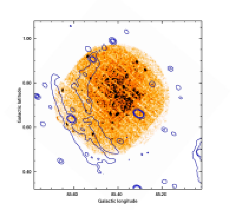
Figure 1.— 0.5–2.5 keV XMM-Newton X-ray mosaic image of G85.4+0.7 with the highest few radio contours overlaid in blue. The X-ray image is Gaussian smoothed with a radius of 3 pixels.

Figure 2.— PN and MOS mosaic images of G85.4+0.7. Top panel: 0.5–2.5 keV image, showing point sources (1-9) and the diffuse emission extraction region, as well as the region used for the central blob (see §7.3). The background region for the diffuse spectra is also shown as a dashed circle. The image is smoothed as in Figure 1. Middle panel: 2.5–10.0 keV image, similarly smoothed and with the same contrast as in the top panel. Bottom panel: 0.5–2.5 keV image, Gaussian smoothed with a radius of 3 pixels and logarithmically scaled and adjusted in contrast to emphasize the diffuse emission and overlaid with contours of the 0.5–2.5 keV emission smoothed similarly to the ROSAT contours in Figure 6 of Kothes et al. (2001).

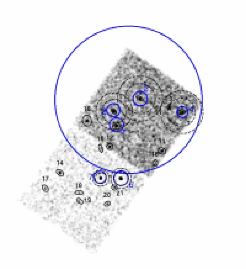
Figure 3.— Chandra image of G85.4+0.7 from the S2 and S3 chips, Gaussian smoothed with a radius of 5 pixels, showing (in black) point source extraction regions and corresponding regions (in blue) for XMM-Newton data for comparison. The large circle indicates the diffuse region in the top panel of Figure 2 and the background regions are shown as dashed circles. (See the online version for colour figure.)

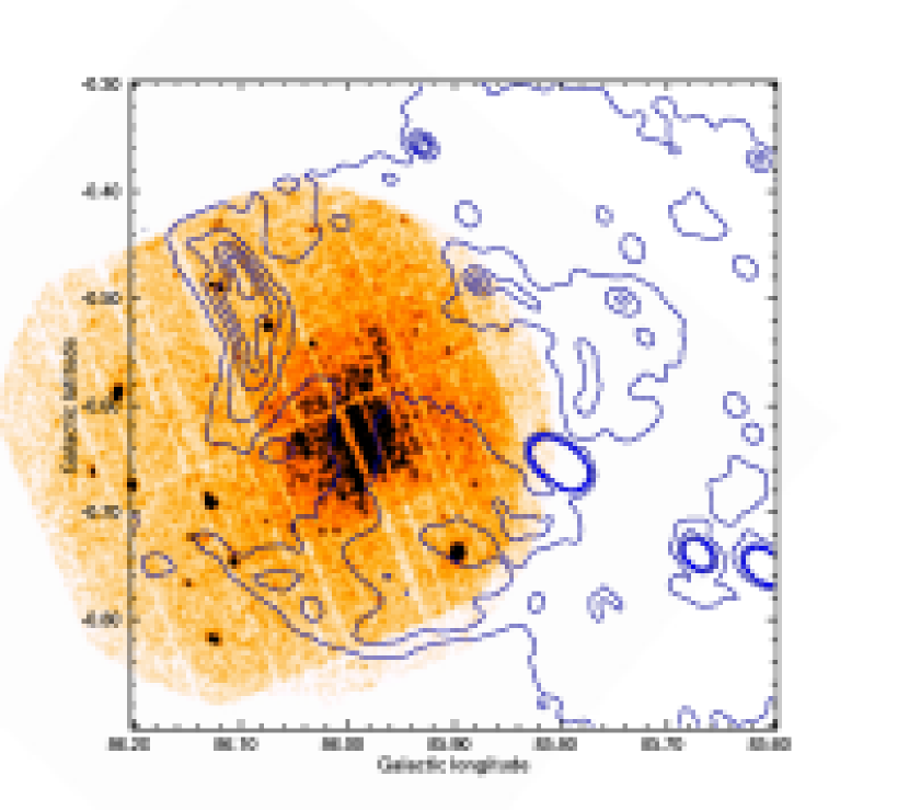
Figure 4.— 0.5–2.5 keV XMM-Newton X-ray mosaic image of G85.9$-$0.6 with the highest few radio contours overlaid in blue. The X-ray image is Gaussian smoothed with a radius of 3 pixels.

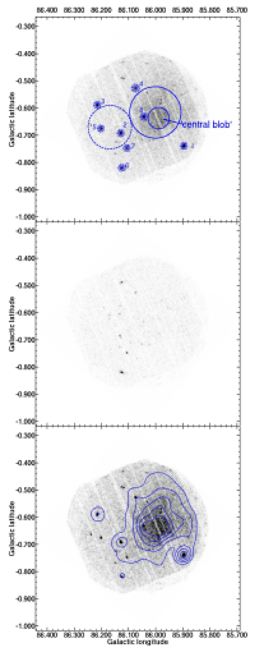
Figure 5.— PN and MOS mosaic images of G85.9$-$0.6. Top panel: 0.5–2.5 keV image, showing point sources (1-8) and the diffuse emission extraction region, as well as the region used for the central blob (see §7.4). The background region for the diffuse spectra is also shown as a dashed circle. The image is smoothed as in Figure 4. Middle panel: 2.5–10.0 keV image, similarly smoothed and with the same contrast as in the top panel. Bottom panel: 0.5–2.5 keV image, Gaussian smoothed with a radius of 3 pixels and logarithmically scaled and adjusted in contrast to emphasize the diffuse emission and overlaid with contours of the 0.5–2.5 keV emission smoothed similarly to the ROSAT contours in Figure 6 of Kothes et al. (2001).

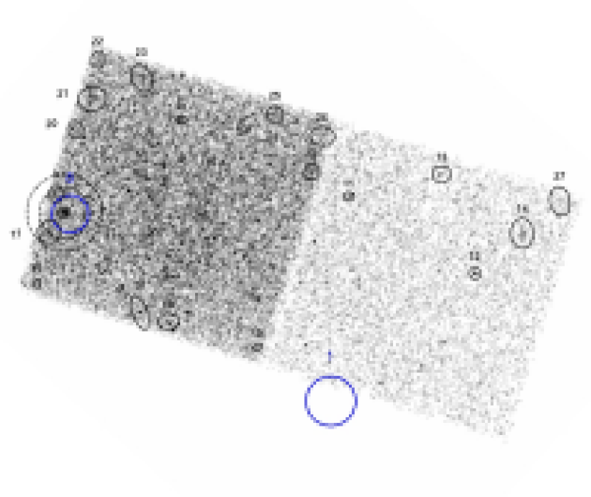
Figure 6.— Chandra image of G85.9$-$0.6 from the S2 and S3 chips, Gaussian smoothed with a radius of 5 pixels. Extraction regions for sources 1 and 8 from the XMM-Newton image are shown as blue circles. (See the online version for colour figure.)

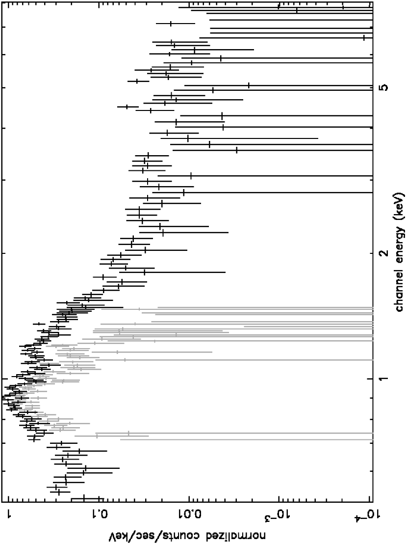
Figure 7.— XMM-Newton PN background subtracted 0.5$-$8.0 keV spectra of G85.4+0.7, using backgrounds from the observation (black) and from blank sky event files (grey). The oversubtraction by the blank sky background is evident. The spectrum using the observation background is clearly background dominated above $\sim$2.5 keV.

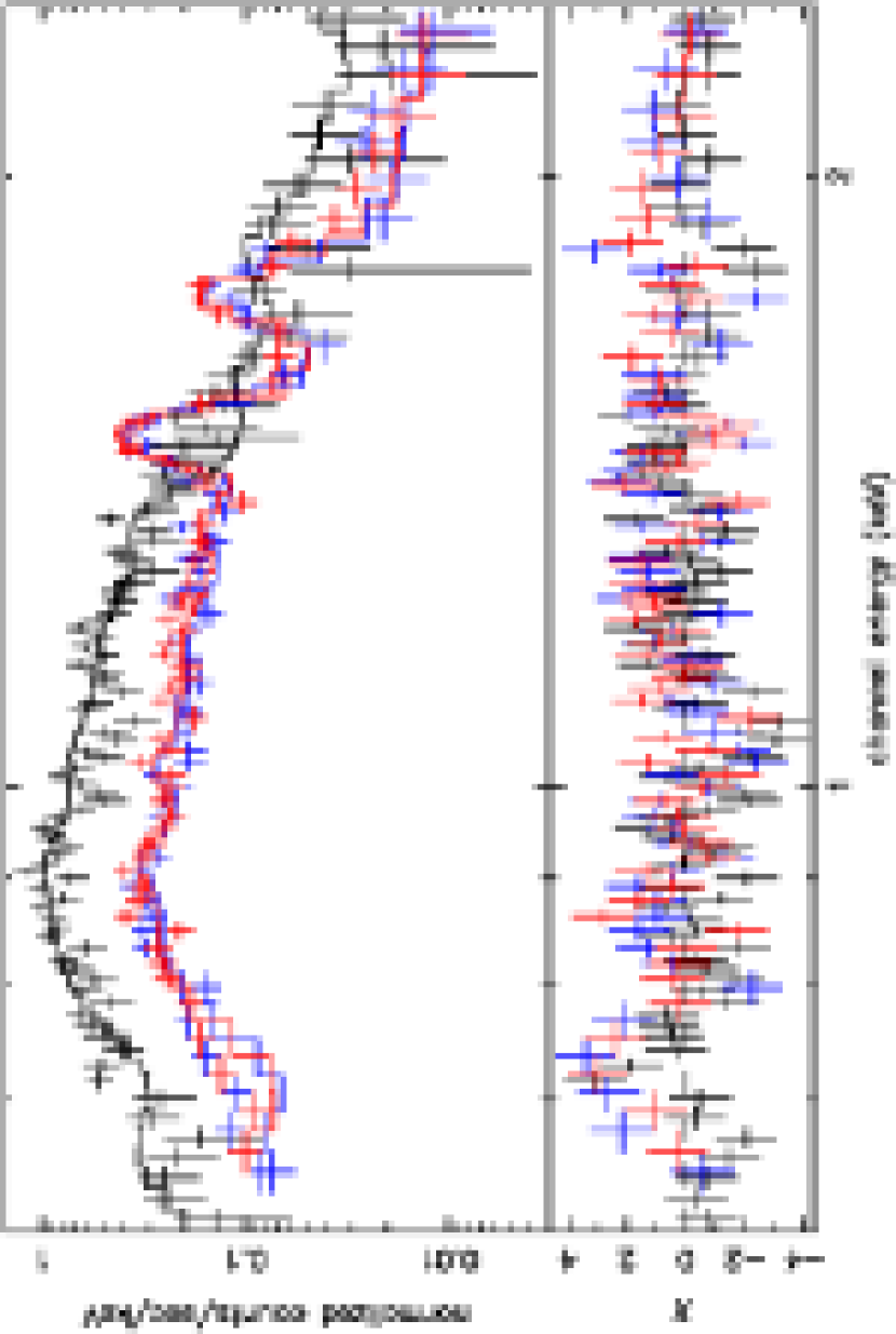
Figure 8.— XMM-Newton PN and MOS 0.5–2.5 keV spectra of G85.4+0.7, fit to an absorbed VPSHOCK. The background spectrum for PN was extracted in the same way as for the spectrum shown in Figure 9 and the background for the MOS instruments are extracted from the XMM-Newton ESAS package described in §4.1. The fitted parameters are given in the third column of Table 1. The PN is shown in black, and the MOS 1 and 2 are shown in blue and red respectively. The bottom panel displays the residuals in units of $\sigma$. Instrumental lines in the MOS spectra appear at 1.49 and 1.75 keV (see §4.1 for details). The line above 1.75 keV is an elemental line which appears in spectra from all instruments.

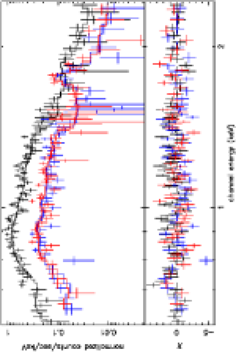
Figure 9.— XMM-Newton PN and MOS spectra of G85.4+0.7, fit to an absorbed VPSHOCK. The background spectra used here were extracted from the region shown in Figure 2. The fitted parameters are given in the second column of Table 1. The PN is shown in black, and the MOS 1 and 2 are shown in blue and red respectively. The bottom panel displays the residuals in units of $\sigma$. An instrumental line in the MOS spectra appears at 1.75 keV (see §4.1 for details).

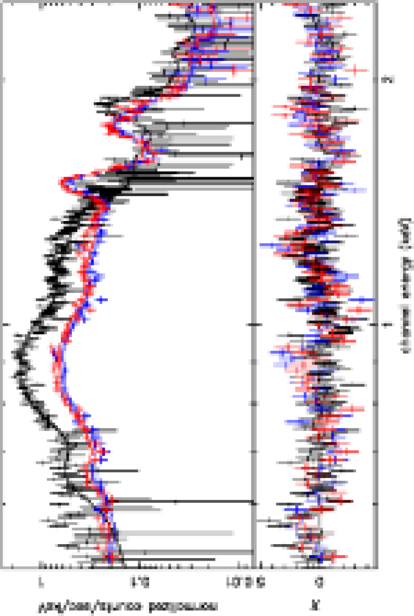
Figure 10.— XMM-Newton PN and MOS 0.5–2.5 keV spectra of G85.9$-$0.6, fit to an absorbed VPSHOCK. The background spectrum for PN was extracted in the same way as for the spectrum shown in Figure 11 and the background for the MOS instruments are extracted from the XMM-Newton ESAS package described in §4.1. The fitted parameters are given in the third column of Table 1. The PN is shown in black, and the MOS 1 and 2 are shown in blue and red respectively. The bottom panel displays the residuals in units of $\sigma$. Instrumental lines in the MOS spectra appear at 1.49 and 1.75 keV (see §4.1 for details). The line above 1.75 keV is an elemental line which appears in spectra from all instruments.

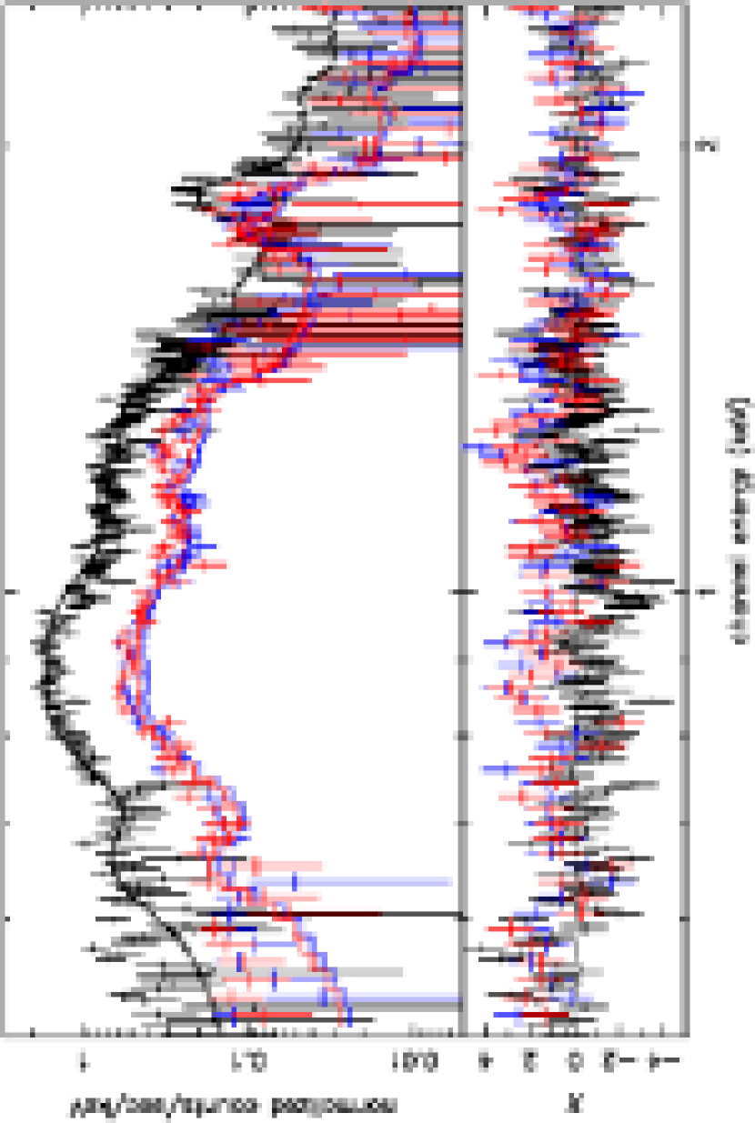
Figure 11.— XMM-Newton PN and MOS 0.5–2.5 keV spectra of G85.9$-$0.6, fit to an absorbed VPSHOCK. The background spectra used here were extracted from the region shown in Figure 5. The fitted parameters are given in the fourth column of Table 1. The PN is shown in black, and the MOS 1 and 2 are shown in blue and red respectively. The bottom panel displays the residuals in units of $\sigma$. An instrumental line in the MOS spectra appears at 1.75 keV (see §4.1 for details). The excess counts in the MOS spectra around 1.4 and 0.85 keV are most likely due to instrumental effects.

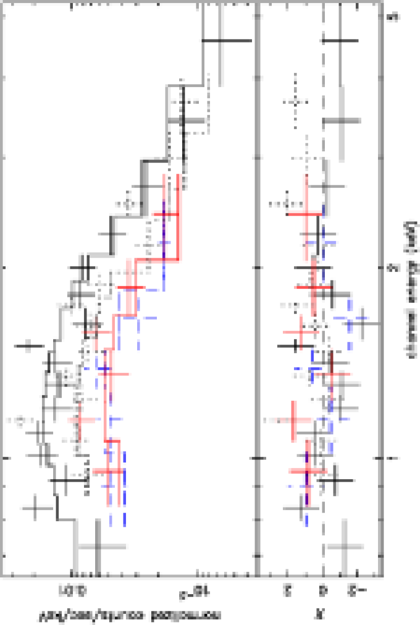
Figure 12.— XMM-Newton PN, MOS, and Chandra 0.5–5 keV spectra of G85.4+0.7 source 1, fit to an absorbed power law. The fitted parameters are given in Table 4. The PN is shown in solid black, the MOS 1 and 2 are shown in dashed blue and solid red respectively, and the Chandra spectrum is shown as dotted black. The bottom panel displays the residuals in units of $\sigma$.

Figure 13.— Integrated foreground hydrogen column density profiles as a function of radial velocity for the two SNRs G85.4+0.7 (left: solid and dotted line) and G85.9$-$0.6 (right: solid line). The dashed lines represent the upper and lower limits for the absorbing H I column density determined from the X-ray spectra. The dotted-dashed line in the diagram for G85.4+0.7 represents the radial velocity of the related stellar wind bubble determined by Kothes et al. (2001).

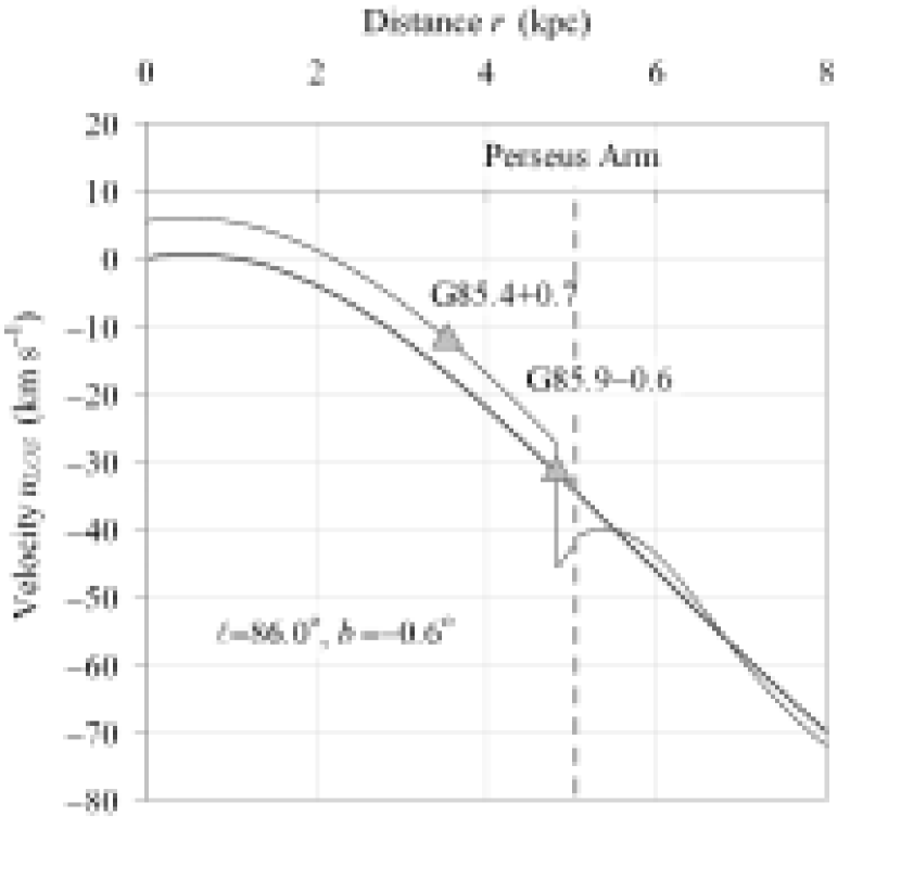
Figure 14.— The velocity field of the H I gas towards $\ell=$86.0$\arcdeg,~{}b=-$0.6$\arcdeg$, from the H I modelling method of Foster & MacWilliams (2006). SNRs G85.4+0.7 & G85.9$-$0.7 are marked with triangles showing their respective distances of 3.5 and 4.8 kpc. The Perseus Spiral arm’s peak density is at 5.0 kpc and the spiral shock that precedes the arm is at 4.8 kpc. The solid dark line is the underlying circular velocity field fitted in this direction, and is a power-law in galactocentric distance (see Foster & MacWilliams, 2006) with a gradient similar to a Schmidt rotation curve.

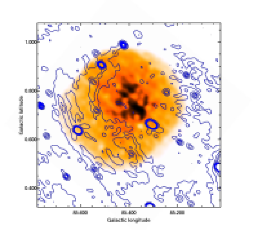
Figure 15.— 0.5–2.0 keV XMM-Newton X-ray mosaic image of G85.4+0.7 with radio contours overlaid in blue. The X-ray image has had the point sources removed and is Gaussian smoothed with a radius of 1^′ to match the radio resolution, in order to compare the radio and diffuse X-ray emission regions. The radio contours were chosen to approximate the appearance of the top image in Figure 2 in Kothes et al. (2001).

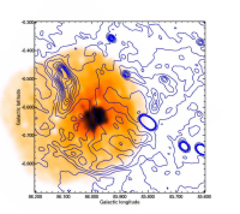
Figure 16.— 0.5–2.5 keV XMM-Newton X-ray mosaic image of G85.9$-$0.6 with radio contours overlaid in blue. The X-ray image has had the point sources removed and is Gaussian smoothed with a radius of 1^′ to match the radio resolution, in order to compare the radio and diffuse X-ray emission regions. The radio contours were chosen to approximate the appearance of the top image in Figure 4 in Kothes et al. (2001).

References

- Borkowski et al. (2001) Borkowski, K. J., Lyerly, W. J., & Reynolds, S. P. 2001 ApJ, 548, 820
- Buccheri et al. (1983) Buccheri, R., et al. 1983, A&A, 128, 245
- Corcoran et al. (2000) Corcoran, M. F., Fredericks, A. C., Petre, R., Swank, J. H., & Drake, S. A. 2000, ApJ, 545, 420
- Cox et al. (1999) Cox, D., Shelton, R. L., Maciejewski, W., Smith, R. K., Plewa, T., Pawl, A., & Ryczka, M. 1999, ApJ, 524, 179
- Dame et al. (1987) Dame, T. M. et al. 1987, ApJ, 322, 706
- Dame et al. (2001) Dame, T. M., Hartmann, D., & Thaddeus, P. 2001, ApJ, 547, 792
- Eisenhauer et al (2005) Eisenhauer, F., et al. 2005, ApJ, 628, 246
- Foster & MacWilliams (2006) Foster, T. & MacWilliams, J. 2006, ApJ, 644, 214
- Gotthelf (2006) Gotthelf, E. V. 2006, in “Young Neutron Stars and Their Environments” (IAU Symposium 218, ASP Conference Proceedings), eds. F. Camilo and B. M. Gaensler. 225
- Guarinos (1992) Guarinos J. 1992, Distribution of interstellar matter in the galactic disk from visual extinction data, in “Astronomy from Large Databases II”, Haguenau 14-16 September 1992, Ed. A. Heck and F. Murtagh, ESO Conference and Workshop Proceedings No 43, ISBN 3-923524-47-1, p. 301
- Harrus et al. (1999) Harrus, I. M., Hughes, J. P., Singh, K. P., Koyama, & Asaoka, I. 1999, ApJ, 488, 781
- Jackson, Safi-Harb, & Kothes (2006) Jackson, M., Safi-Harb, S., & Kothes, R. 2006 Canadian Astronomical Society Meeting, Calgary, Canada, June 1-4
- Kothes et al. (2001) Kothes, R., Landecker, T. L., Foster, T., and Leahy, D. A. 2001, A&A, 376, 641
- Leahy, Elsner, & Weisskopf (1983) Leahy, D. A., Elsner, R. F., & Weisskopf, M. C. 1983, ApJ, 272, 256
- Liedahl et al. (1990) Liedahl, D. A., Kahn, S. M., Osterheld, A. L., & Goldstein, W. H. 1990, ApJ, 350, L37
- Lumb (2002) Lumb, D. 2002, EPIC Background Files, XMM-SOC-CAL-TN-0016, Issue 2.0, http://xmm.vilspa.esa.es/docs/documents/CAL-TN-0016-2-0.ps.gz
- Lyne & Graham-Smith (1998) Lyne, A. G., & Graham-Smith, F. 1998, Pulsar Astronomy, Cambridge: Cambridge University Press.
- Mewe et al. (1985) Mewe, R., Gronenschild, E. H. B. M., & van den Oord, G. H. J. 1985, A&AS, 62, 197
- Mewe et al. (2003) Mewe, R., Raasssen, A. J. J., Cassinelli, J. P., van der Hucht, K. A., Miller, N. A., & Güdel, M. 2003 A&A, 398, 203 ,& van den Oord, G. H. J. 1985, A&AS, 62, 197
- Monet et al. (1998) Monet, D., et al. 1998, USNO-A V2.0, A Catalog of Astrometric Standards
- Monet et al. (2003) Monet, D. G., et al. 2003, AJ, 125, 948
- Morrison & McCammon (1983) Morrison, R., & McCammon, D. 1983, ApJ, 270, 119
- Myers et al. (2002) Myers J.R., Sande C.B., Miller A.C., Warren Jr. W.H., Tracewell D.A. 2002, SKY2000 Master Catalog, Version 4
- Read & Ponman (2003) Read A.M. & Ponman T.J., 2003, A&A, 409, 395
- Rho & Petre (1997) Rho, J., & Petre, R. 1997, ApJ, 484, 828
- Roberts (1969) Roberts, W. W. 1969, ApJ, 158, 123
- Rohlfs & Wilson (2004) Rohlfs, K. & Wilson. T. L. 2004, “Tools of Radio Astronomy”, 4th rev. & enl. ed., Berlin: Springer, 2004
- Safi-Harb (2006) Safi-Harb, S. 2006, American Astronomical Society, 208, #61.03
- Safi-Harb et al. (2005) Safi-Harb, S., Dubner, G., Petre, R., Holt, S. S., & Durouchoux, P. 2005, ApJ, 618, 321
- Skrutskie et al. (2006) Skrutskie, M. F., et al. 2006, AJ, 131, 1163
- Snowden & Kuntz (2006) Snowden, S. L. & Kuntz, K. D., 2006. Cookbook for Analysis Procedures for XMM-Newton EPIC MOS Observations of Extend Objects and the Diffuse Background, Version 1.0.1.
- Strüder et al. (2001) Strüder, L., et al. 2001, A&A, 365, L18
- Taylor et al. (2003) Taylor, A. R. et al. 2003, AJ, 125, 3145.
- Townsley et al. (2000) Townsley, L. K., Broos, P. S., Garmire, G. P., Nousek, J. A., 2000, ApJ, 534, L139
- Turner et al. (2001) Turner, M. J. L., et al. 2001, A&A, 365, L27
- White & Long (1991) White, R. L. & Long, K. S. 1991, ApJ, 373, 543
- Wielen (1979) Wielen, R. 1979, in IAU Symp. 84, The Large-Scale Characteristics of the Galaxy, ed. W. B. Burton (Dordrecht: Reidel), 133
- Woods & Thompson (2006) Woods, P. & Thompson, C. 2006 in “Compact Stellar X-ray Sources”, eds. W. Lewin & M. van der Klis (Cambridge: Cambridge University Press), 547