Status of the MILC light pseudoscalar meson project

Abstract:

We discuss the current status of our calculation of the physics of $\pi$ and $K$ mesons using three dynamical flavors of improved staggered quarks. This year, we have a new ensemble with a lattice spacing of $0.06\;$fm and a light sea mass of $0.2m_{s}$, as well as significant increases in statistics at several coarser lattice spacings and/or heavier sea masses. Results for decay constants, quark masses, low energy constants, condensates, and $V_{us}$ are presented.

We are using improved staggered quarks [1] with $N_{f}=3$ dynamical flavors (both unquenched (“full”) QCD and partially quenched) to study the physics of light pseudoscalars ($\pi$, $K$). Since our original published work [2], we have continued to add data sets with lighter sea quark masses and/or finer lattice spacings and to improve the analysis. This is the latest in a series of periodic updates [3, 4]. We concentrate here on those aspects that have changed since last year.

Table 1 gives the parameters of our lattices. The quantities $m^{\prime}_{s}$ and $\hat{m}^{\prime}\!=\!m^{\prime}_{u}\!=\!m^{\prime}_{d}$ denote the values of sea quark masses chosen in each run. (The corresponding masses without the primes, e.g., $m_{s}$ and $\hat{m}\equiv(m_{u}+m_{d})/2$, are the physical values.)

$a$ (fm)	$a\hat{m}^{\prime}$ / $am^{\prime}_{s}$	$L$ (fm)	$m_{\pi}$ / $m_{\rho}$	$m_{\pi}L$	$10/g^{2}$	Lat Dim	# Lats
$\approx\!0.15$	0.0290 / 0.0484	2.4	0.522	6.7	6.600	$16^{3}\times 48$	600
$\approx\!0.15$	0.0194 / 0.0484	2.4	0.454	5.5	6.586	$16^{3}\times 48$	600
$\approx\!0.15$	0.0097 / 0.0484	2.4	0.348	3.9	6.572	$16^{3}\times 48$	600
$\approx\!0.15$	0.00484 / 0.0484	3.0	0.256	3.4	6.566	$20^{3}\times 48$	600
$\approx\!0.12$	0.03 / 0.05	2.4	0.582	7.6	6.81	$20^{3}\times 64$	362
$\approx\!0.12$	0.02 / 0.05	2.4	0.509	6.2	6.79	$20^{3}\times 64$	485
$\approx\!0.12$	0.01 / 0.05	2.4	0.394	4.5	6.76	$20^{3}\times 64$	894
$\approx\!0.12$	0.01 / 0.05	3.4	0.395	6.3	6.76	$28^{3}\times 64$	275
$\approx\!0.12$	0.007 / 0.05	2.4	0.342	3.8	6.76	$20^{3}\times 64$	836
$\approx\!0.12$	0.005 / 0.05	2.9	0.299	3.8	6.76	$24^{3}\times 64$	527
$\approx\!0.12$	0.03 / 0.03	2.4	0.590	7.6	6.81	$20^{3}\times 64$	360
$\approx\!0.12$	0.01 / 0.03	2.4	0.398	4.5	6.76	$20^{3}\times 64$	349
$\approx\!0.09$	0.0124 / 0.031	2.4	0.495	5.8	7.11	$28^{3}\times 96$	531
$\approx\!0.09$	0.0062 / 0.031	2.4	0.380	4.1	7.09	$28^{3}\times 96$	583
$\approx\!0.09$	0.0031 / 0.031	3.4	0.297	4.2	7.08	$40^{3}\times 96$	503
$\approx\!0.06$	0.0072 / 0.018	2.9	0.474	6.3	7.48	$48^{3}\times 144$	556
$\approx\!0.06$	0.0036 / 0.018	2.9	0.370	4.5	7.47	$48^{3}\times 144$	334

Table 1: Lattice parameters. The lattice spacings are the “nominal” scales (see text). The $\pi$ and $\rho$ referred to are those formed out of the sea quarks for each lattice; valence quark masses however go down to the lightest sea-quark values in the table.

The $a\!\approx\!0.06\;$fm lattice with masses 0.0036 / 0.018 is a new ensemble this year, as is (for this analysis) the large-volume $a\!\approx\!0.12\;$fm lattice with masses 0.01 / 0.05 and spatial size $28^{3}$. The numbers of configurations for the $a\!\approx\!0.06\;$fm lattice with masses 0.0072 / 0.018 and for several of the $a\!\approx\!0.12\;$fm lattices have almost doubled since last year. Running on an $a\!\approx\!0.06\;$fm lattice with $\hat{m}^{\prime}=0.1m_{s}^{\prime}$ (masses 0.0018 / 0.018) has recently begun but is not included here.

On each ensemble, we determine $r_{1}/a$, where $r_{1}(\hat{m}^{\prime},m_{s}^{\prime},g^{2})$ [5] is a length scale from the static quark potential, similar to $r_{0}$ [6]. The quantity $r_{1}^{\rm phys}$, defined as the continuum $r_{1}$ at physical quark masses ($\hat{m}$, $m_{s}$) may be determined from the $r_{1}/a$ values and the $\Upsilon$ 2S-1S splitting [7]. We obtain $r_{1}^{\rm phys}=0.318(7)\;$fm [4, 8].

For generic chiral and continuum extrapolations, it is convenient to define the lattice scale by $a\equiv r_{1}^{\rm phys}/(r_{1}(\hat{m}^{\prime},m_{s}^{\prime},g^{2})/a)$. We call this the “nominal” scale-setting procedure. In choosing the input lattice coupling $g^{2}$, we kept $r_{1}/a$ fixed as $\hat{m}^{\prime}$ and $m_{s}^{\prime}$ changed over a given set of ensembles (e.g., the $a\!\approx\!0.12\;$fm ensembles). Thus, up to tuning errors, each ensemble grouped within a box in Table 1 has the same nominal scale. However, fixing the scale this way is not completely correct for applying chiral perturbation theory ($\chi$PT) to quantities such as $f_{\pi}$ since $r_{1}$ has some (small, but physical) dependence on the dynamical quark masses that is not included in $\chi$PT.

A mass-independent procedure to set the scale is preferable [9]. A convenient procedure is to replace $r_{1}(\hat{m}^{\prime},m_{s}^{\prime},g^{2})/a$ by $r_{1}(\hat{m},m_{s},g^{2})/a$, where the value of $r_{1}(\hat{m},m_{s},g^{2})/a$ at physical masses $\hat{m},m_{s}$ is obtained by a smooth interpolation/extrapolation from $r_{1}(\hat{m}^{\prime},m_{s}^{\prime},g^{2})/a$. We tried this mass-independent scheme in Ref. [2], but the differences with the nominal approach were smaller than other systematic errors for all quantities. With better data, we now find significant differences in a few low energy constants (LECs). In addition, the mass-independent scheme tends to have better confidence levels in our $\chi$PT fits. Therefore we use this scheme exclusively here.

As in Refs. [2, 3, 4] we fit the partially quenched (PQ) lattice data to rooted staggered chiral perturbation theory (rS$\chi$PT) forms [10, 11, 12]. We always fit multiple lattice spacings, and both masses and decay constants, simultaneously. To determine the LO and NLO LECs and chiral-limit quantities, we fit to the low quark-mass region, and omit the $a\!\approx\!0.15\;$fm lattices, where taste violations are large. Denoting the valence quark masses in the mesons by $m_{x}$ and $m_{y}$, the low-mass cuts are: $am_{x}+am_{y}{\,\raise 1.29167pt\hbox{$<$\kern-7.5pt\lower 4.30554pt\hbox{$\sim$}}\,}0.39\;am_{s}$ (at $a\!\approx\!0.12\;$fm); $am_{x}+am_{y}{\,\raise 1.29167pt\hbox{$<$\kern-7.5pt\lower 4.30554pt\hbox{$\sim$}}\,}0.51\;am_{s}$ (at $a\!\approx\!0.09\;$fm); and $am_{x}+am_{y}{\,\raise 1.29167pt\hbox{$<$\kern-7.5pt\lower 4.30554pt\hbox{$\sim$}}\,}0.56\;am_{s}$ (at $a\!\approx\!0.06\;$fm). We can tolerate a higher cutoff at smaller lattice spacing because the taste violations, and hence the masses of non-Goldstone pions, are smaller. In these fits, we also cut on sea-quark mass and remove the $a\!\approx\!0.12\;$fm sets with masses $0.03/0.05$, $0.02/0.05$, and $0.03/0.03$. Because the statistical errors are so small, we still need to add in the NNLO analytic terms to the complete NLO forms in order to get good fits [2].

For interpolation around $m_{s}$, we must include higher quark masses. Once LO and NLO parameters are determined, we fix them (up to statistical errors) and fit to all sea mass sets, all lattice spacings, and valence masses $m_{x}+m_{y}{\,\raise 1.29167pt\hbox{$<$\kern-7.5pt\lower 4.30554pt\hbox{$\sim$}}\,}1.2\;m_{s}$. We now also need to add in NNNLO analytic terms to get good fits. These NNNLO fits are used for central values of $f_{\pi}$, $f_{K}$ and quark masses.

Figure 1 shows results for the squared pseudoscalar masses as a function of quark mass. “Pions” have valence masses $m_{y}=m_{x}$; while “kaons” have $m_{y}$ held fixed at various (arbitrary) values while $m_{x}$ varies. The fit is to the full quark-mass range and uses NNNLO terms.

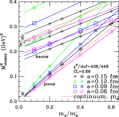
Figure 1: Comparison of NNNLO fit to partially-quenched squared meson masses. For clarity only the lightest sea-quark ensemble for each lattice spacing is shown.

For the pions, the relative values of the results on various lattices is determined largely by the relation between the simulation strange mass $m_{s}^{\prime}$ in the sea and the physical mass $m_{s}$. For example, $m_{s}^{\prime}/m_{s}$ is largest for the $a\!\approx\!0.12\;$fm lattices, which makes the slope of the pion data greatest for these lattices. For kaons, the biggest effect is simply the choice of the values of the fixed valence mass $m_{y}$, typically chosen to be various fixed fractions of $m_{s}^{\prime}$.

Extrapolating to the continuum and setting valence and sea quark masses equal, we get the dashed red lines; $m_{s}^{\prime}$ has been adjusted so that both the kaon and the pion hit their physical values at the same value of $m_{x}$. This gives the physical quark masses $\hat{m}$ and $m_{s}$ (after renormalization).

Note that the fit lines in Fig. 1 are remarkably straight on this scale. To see curvature coming from the NLO chiral logs as well as the analytic higher order terms, we plot $m_{\pi}^{2}/(m_{x}+m_{y})$ in Fig. 2 (left). As the lattice spacing decreases, the PQ log at small mass becomes more evident. At larger lattice spacing, the PQ log is largely washed out by staggered taste violations. The continuum dashed red line has sea and valence masses equal, so no PQ log is expected.

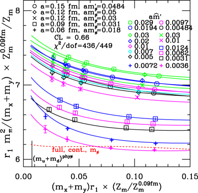
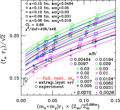
Figure 2: Data for $m_{\pi}^{2}/(m_{x}+m_{y})$ is plotted at left; while that for $f_{\pi}$ is plotted at right. This is the same fit as in Fig. 1. All sea-quark ensembles are represented, but only “pion” points ($m_{x}\!=\!m_{y}$) are shown.

In Fig. 2 (right), we show the behavior of the decay constant. Extrapolating to the continuum, setting $m^{\prime}_{s}=m_{s}$, and setting light valence and sea masses equal gives the dashed red line. The final result for $f_{\pi}$ after extrapolating $m_{x},m_{y}\!\to\!\hat{m}$ is marked by a $+$. The experimental result is indicated by the $\circ$; it comes from the $\pi^{+}\to\mu^{+}+\nu_{\mu}$ decay width and $V_{ud}=0.97377(27)$ [13].

All points and fit lines above have been corrected for finite volume effects using the rS$\chi$PT forms at one loop. However, it is known [14] that finite volume effects coming from higher orders in $\chi$PT can be a large ($\sim\!50\%$) correction to the one-loop effects in the current ranges of quark mass and volume. We therefore study this issue directly by comparing results on the spatial size $20^{3}$ and $28^{3}$ $a\!\approx\!0.12\;$fm ensembles with $a\hat{m}^{\prime}=0.01$, $am_{s}^{\prime}=0.05$. These lattices have spatial length $2.4\;$fm and $3.4\;$fm, respectively. The comparison is shown in Table 2.

quantity	% difference	boosted % diff.	1-loop % diff.
$af_{\pi}$	1.4(2)%	1.6(2)%	1.1%
$af_{K}$	0.4(3) %	0.4(3) %	0.3%
$(am_{\pi})^{2}$	-1.0(4)%	-1.2(4)%	-0.9%
$(am_{K})^{2}$	-0.4(2) %	-0.4(2) %	-0.2%

Table 2: Finite volume effects. The second column is the % difference between the values on the $28^{3}$ and the $20^{3}$ lattice. In the third column, we “boost” the difference, to take into account the (small) further difference between $28^{3}$ and infinite volume. (We use one-loop results to make the adjustment.) The last column shows the % difference between $20^{3}$ and infinite volume as predicted by one-loop rS$\chi$PT. “Pion” quantities are from lattice valence masses $0.005$, $0.005$; “kaon” quantities are from lattice valence masses $0.005$, $0.04$.

As expected from Ref. [14], the true finite volume effects are larger than those predicted at one-loop, although only for $f_{\pi}$ are the relative errors small enough to make the comparison unambiguous. We define the “residual finite volume effect” on the $20^{3}$ lattice as that effect not taken into account at one-loop, i.e., the difference between columns three and four in Table 2. In practice, the $20^{3}$, $a\hat{m}^{\prime}=0.01$, $am_{s}^{\prime}=0.05$, $a\!\approx\!0.12\;$fm lattice is close to the worst case in our data set, since the volumes both at the lightest sea quark masses and at the finest lattice spacings are larger.

Judging by the one-loop results, we expect the overall (and hence residual) finite volume effects closest to the chiral and continuum limits in our data set to be about half those seen in the table. We therefore correct our data by $1/2$ the residual finite volume effects from Table 2, and take the full size of the correction as a systematic error. We note that the size of the error determined here is very similar to that estimated by us previously [2] using Ref. [14].

The fact that we can get good fits to the forms predicted by rS$\chi$PT (and not to those of continuum $\chi$PT [2]) is an overall test of staggered chiral perturbation theory, including the “replica trick” to represent rooting. As a more focused test of the replica trick in rS$\chi$PT, we allow $n_{r}$, the number of replicas per staggered flavor, to be a free fit parameter. If rS$\chi$PT is correct, we should find $n_{r}=1/4$. On the low-mass data set described above, we obtain $n_{r}=0.28(2)(3),$ where the errors are statistical and systematic (describing the variation over details of the chiral fits). While the ability of rS$\chi$PT to describe rooted staggered data cannot prove the correctness of the rooting trick itself, it does indicate that no problems occur in the chiral sector of the rooted theory [12]. This is because rS$\chi$PT reproduces continuum $\chi$PT in the limit $a\to 0$.

Using $r_{1}=0.318(7)\;$fm from $\Upsilon$ splittings, we obtain (still preliminary)

$$f_{\pi} = 128.3\pm 0.5\;{}^{+2.4}_{-3.5}\;{\rm Me\!V}$$

$$f_{K} = 154.3\pm 0.4\;{}^{+2.1}_{-3.4}\;{\rm Me\!V}$$

$$f_{K}/f_{\pi} = 1.202(3)({}^{+\phantom{1}8}_{-14})\ ,$$

where the errors are from statistics and lattice systematics. These results are consistent with our previous results [2], with 20–30% smaller errrors. Our value for $f_{\pi}$ is consistent with the experimental result, $f_{\pi}^{\rm expt}=130.7\pm 0.1\pm 0.36\;{\rm Me\!V}$ [13].

Instead of setting the scale from $\Upsilon$ splittings, we can set the scale from $f_{\pi}$ itself, which gives smaller errors for $\pi$–$K$ quantities. Note that even dimensionless quantities can change with the new scale, due to changes in physical quark masses. We then obtain (preliminary):

$$f_{K}=156.5\pm 0.4\;{}^{+1.0}_{-2.7}\;{\rm Me\!V} f_{K}/f_{\pi}=1.197(3)({}^{+\phantom{1}6}_{-13})$$

$$f_{\pi}/f_{2}=1.052(2)({}^{+6}_{-3}) \langle\bar{u}u\rangle_{2}=-(\,278(1)({}^{+2}_{-3})(5)\;{\rm Me\!V}\,)^{3}$$

$$f_{\pi}/f_{3}=1.21(5)({}^{+13}_{-\phantom{1}3}) \langle\bar{u}u\rangle_{3}=-(\,242(9)({}^{+\phantom{2}5}_{-17})(4)\;{\rm Me\!V}\,)^{3}$$

$$f_{2}/f_{3}=1.15(5)({}^{+13}_{-\phantom{1}3}) \langle\bar{u}u\rangle_{2}/\langle\bar{u}u\rangle_{3}=1.52(17)({}^{+38}_{-15})$$

$$2L_{6}-L_{4}=0.4(1)({}^{+2}_{-3}) 2L_{8}-L_{5}=-0.1(1)(1)$$

$$L_{4}=0.4(3)({}^{+3}_{-1}) L_{5}=2.2(2)({}^{+2}_{-1})$$

$$L_{6}=0.4(2)({}^{+2}_{-1}) L_{8}=1.0(1)(1)$$

$$m_{s}=88(0)(3)(4)(0)\;{\rm Me\!V} \hat{m}=3.2(0)(1)(2)(0)\;{\rm Me\!V}$$

$$m_{u}=1.9(0)(1)(1)(1)\;{\rm Me\!V} m_{d}=4.6(0)(2)(2)(1)\;{\rm Me\!V}$$

$$m_{s}/\hat{m}=27.2(1)(3)(0)(0) m_{u}/m_{d}=0.42(0)(1)(0)(4)\;.$$

The errors are statistical, lattice-systematic, perturbative (for masses and condensates; from two-loop perturbation theory [15]) and electromagnetic (for masses; from continuum estimates). $f_{2}$ ($f_{3}$) represents the three-flavor decay constant in the two (three) flavor chiral limit, and $\langle\bar{u}u\rangle_{2}$ ($\langle\bar{u}u\rangle_{3}$) is the corresponding condensate. The low energy constants $L_{i}$ are in units of $10^{-3}$ and are evaluated at chiral scale $m_{\eta}$; the condensates and masses are in the ${\overline{\rm MS}}$ scheme at scale $2\,{\rm Ge\!V}$.

We also obtain

$$r_{1}=0.3108(15)({}^{+26}_{-79})\;{\rm fm}\ ,\vspace{-1mm}$$

which is 1-$\sigma$ lower (and with somewhat smaller errors) than the value from the $\Upsilon$ system. There is a 2-$\sigma$ conflict between our $r_{1}$ result from $f_{\pi}$ and the HPQCD Collaboration [7] value from $\Upsilon$ splittings, $r_{1}=0.321(5)\;$fm. If instead we compare to our own evaluation of $r_{1}$ from the $\Upsilon$ spectrum, $r_{1}=0.318(7)$ [4], the difference is only $1$-$\sigma$. We emphasize, however, that the evaluations of $r_{1}$ from the $\Upsilon$ splittings both by us and by the HPQCD Collaboration use the same lattice data: HPQCD $\Upsilon$ splittings [7] and MILC values of $r_{1}/a$ [8]. The difference is only in how we extrapolate to the physical point and estimate the systematic error. Our result is consistent, though, with the ($N_{f}=2$) result from the ETM Collaboration [16], $r_{0}=0.454(7)\;$fm. Converting from $r_{0}$ to $r_{1}$ using the ratio $r_{0}/r_{1}=1.46(1)(2)$ (from Ref. [8], adjusted for the slight difference between $N_{f}=3$ and $N_{f}=2$), this gives $r_{1}=0.311(7)\;$fm.

Together with the experimental result for the kaon leptonic branching fraction [17], our result for $f_{K}/f_{\pi}$ implies $|V_{us}|=0.2246({}^{+25}_{-13})$, which is consistent with (and competitive with) the world-average value $|V_{us}|=0.2257(21)$ [13] coming from semileptonic $K$-decay coupled with non-lattice theory.

The change in the perturbative mass renormalization constant $Z_{m}$ from one to two loops accounts for almost all of the difference between the mass values quoted here and those in Ref. [18, 2]. A non-perturbative evaluation of $Z_{m}$ is in progress.

We stress that our extraction of the $L_{i}$ uses fits that include (analytic) NNLO terms. Therefore, a comparison to other evaluations, either phenomenological or on the lattice, that stop at NLO terms is problematic. Indeed, NNLO terms of “natural size” in $\chi$PT can produce changes in the $L_{i}$ (relative to a pure NLO evaluation) that are as large as, or even somewhat larger than, our current systematic errors. This is confirmed by NLO fits to our data. Such fits have very poor confidence levels, however, which is why we do not include them in the analysis.

The $SU(2)_{L}\times SU(2)_{R}$ LECs $\bar{l}_{3}$, $\bar{l}_{4}$ that are extracted [19] from our $SU(3)_{L}\times SU(3)_{R}$ results using one-loop (NLO) formulae are therefore quite sensitive to the NNLO terms, particularly for $\bar{l}_{3}$. An NLO fit, on the other hand, gives $\bar{l}_{3}=2.85(7)$ (statistical errors only), which is comparable to the results from groups [16, 20] performing two-flavor simulations with NLO $SU(2)_{L}\times SU(2)_{R}$ fits. Indeed, this must be true, because the $m_{\pi}^{2}$ data are so linear (see Fig. 1), which requires $\bar{l}_{3}$ to have roughly this value [19]. Alternative fits using $SU(2)_{L}\times SU(2)_{R}$ rS$\chi$PT are in progress. Since the strange sea-quark is omitted from the chiral theory, the approach should make possible good NLO fits on light-mass data, and thereby bypass this issue. Inclusion of two-loop (continuum) chiral logs [21] in $SU(3)_{L}\times SU(3)_{R}$ fits is also in progress.

This work is supported in part by the US DoE and NSF. Computations were performed at the NSF Teragrid, NERSC, and USQCD centers, and at computer centers at the University of Arizona, the University of California at Santa Barbara, Indiana University, and the University of Utah.

References

- [1] K. Orginos, D. Toussaint and R.L. Sugar, Phys. Rev. D 60 (1999) 054503 and references therein.
- [2] C. Aubin et al. [MILC Collaboration], Phys. Rev. D 70, 114501 (2004).
- [3] C. Aubin et al. [MILC Collaboration], Nucl. Phys. B (Proc. Suppl.) 140 (2005) 231.
- [4] C. Bernard et al. [MILC Collaboration], PoS LAT2005, 025, (2005), hep-lat/0509137; PoS LAT2006, 163, (2006), hep-lat/0609053; and hep-lat/0611024, to be published in the proceedings of Chiral Dynamics 2006, Duke University, Sept. 18-22, 2006.
- [5] C. Bernard et al. [MILC Collaboration], Phys. Rev. D 62, 034503 (2000).
- [6] R. Sommer, Nucl. Phys. B411, 839 (1994).
- [7] A. Gray et al. [HPQCD Collaboration], Phys. Rev. D 72, 094507 (2005).
- [8] C. Aubin et al. [MILC Collaboration], Phys. Rev. D 70, 094505 (2004).
- [9] R. Sommer et al. [ALPHA Collaboration], Nucl. Phys. Proc. Suppl. 129, 405 (2004).
- [10] W. Lee and S. Sharpe Phys. Rev. D 60, 114503 (1999); C. Bernard, Phys. Rev. D 65, 054031 (2002).
- [11] C. Aubin and C. Bernard, Phys. Rev. D 68, 034014 (2003) and Phys. Rev. D 68, 074011 (2003).
- [12] C. Bernard, Phys. Rev. D 73, 114503 (2006); C. Bernard, M. Golterman, and Y. Shamir, presented at the International Symposium, Lattice 2007, Regensburg, Germany, July 30–Aug. 4, 2007, PoS LAT2007, 263, arXiv:0709.2180[hep-lat] and in preparation.
- [13] W.-M. Yao et al. [Particle Data Group], Journal of Physics G 33, 1 (2006) and 2007 partial update.
- [14] G. Colangelo, S. Dürr and C. Haefeli, Nucl. Phys. B 721, 136 (2005).
- [15] Q. Mason et al. [HPQCD Collaboration], Phys. Rev. D 73, 114501 (2006).
- [16] Ph. Boucaud et al. [ETM Collaboration], Phys. Lett. B 650, 304 (2007).
- [17] F. Ambrosino et al. [KLOE Collaboration], Phys. Lett. B 632, 76 (2006).
- [18] C. Aubin et al. [HPQCD, MILC, and UKQCD Collaborations], Phys. Rev. D 70, 031504(R) (2004).
- [19] H. Leutwyler, arXiv:0706.3138 [hep-ph].
- [20] L. Del Debbio et al., JHEP 0702, 056 (2007) and JHEP 0702, 082 (2007).
- [21] J. Bijnens, N. Danielsson and T. A. Lahde, Phys. Rev. D 73, 074509 (2006).