Supplementary Material

Supplementary Information

Online material: Heavy electrons and the symplectic symmetry of spin

Rebecca Flint, M. Dzero and P. Coleman

Center for Materials Theory, Rutgers University, Piscataway, NJ 08855, U.S.A.

I Online material in theory papers in Nature and Science.

The past decade has seen the rise in importance of high impact science journals like Science, Nature and its spectrum of associated journals, Nature Physics, Photonics and Materials. Funding agencies increasingly look to measure physicists’ performance by the articles they have published in these high impact journals.

The established format for papers in these high impact journals tends to minimize the number of mathematical equations, favoring a more conceptual and richly colored figure-based representation of key results. This format is ideal for experimental papers, but puts theoretical papers that rely on the language of mathematics at a disadvantage. We believe that the supporting online materials that accompany Science and Nature articles can provide a new format that can help redress this balance. More mathematical theory papers that are submitted to these journals can now be written with the main conceptual results in the body of the paper, accompanied by key computations and appendix material online. Of course, such material can, in the course of time, be groomed for publication in a longer article, but in the mean time, this provides a mechanism for key theory papers to be published in high impact journals.

The online material presented here provides the background material for reproducing our results. We have given an introduction to symplectic spins, and a full derivation of the the application of symplectic N to the new heavy electron superconductors $PuCoGa_{5}$ and $NpPd_{5}Al_{2}$. We have also included a brief section describing the test-bed application of this same method to frustrated magnetism.

II Symplectic spins

II.1 N-dimensional Symplectic Pauli Matrices

Symplectic spin operators form a subset of the generators of the $SU(N)$ group. To determine their general form, we simply project out the component $S$ of the $SU(N)$ spin generators which reverses under time-reversal, i.e the components $S$ for which $\hat{\epsilon}S^{T}\hat{\epsilon}^{T}=-S$. For even $N$, the fundamental $SU(N)$ spin generators can be written

$$[{\cal T}^{pq}]_{\alpha\beta}=\delta^{p}_{\alpha}\delta^{q}_{\beta}-\frac{1}{N}\delta^{pq}\delta_{\alpha\beta}.$$ (1)

Here, all indices range over $[\pm 1,\pm k]$, (excluding zero) where $N=2k$ is even. The general symplectic spin operator is obtained by subtracting the time-reversed $SU(N)$ generator $\hat{\epsilon}{\cal T}^{T}\hat{\epsilon}^{T}$ from $\cal T$, $S^{pq}={\cal T}^{pq}-\hat{\epsilon}[{\cal T}^{pq}]^{T}\hat{\epsilon}^{T}$. Putting $[\hat{\epsilon}]^{\alpha}_{\beta}=\tilde{\alpha}\delta^{\alpha}_{-\beta}$, where $\tilde{\alpha}={\rm sgn}(\alpha)$, then

$$[S^{pq}]_{\alpha\beta}=\delta^{p}_{\alpha}\delta^{q}_{\beta}-\epsilon^{p}_{\beta}\epsilon^{q}_{\alpha}=\delta^{p}_{\alpha}\delta^{q}_{\beta}-\tilde{\alpha}\tilde{\beta}\delta^{p}_{-\beta}\delta^{q}_{-\alpha}.$$ (2)

This traceless matrix satisfies $S^{pq}=-\hat{\epsilon}[S^{pq}]^{T}\hat{\epsilon}^{T}$, or $S^{pq}_{\alpha\beta}=-\tilde{\alpha}\tilde{\beta}S^{pq}_{-\beta-\alpha}$. Since $S^{pq}=-\tilde{p}\tilde{q}S^{{-q\ -p}}$, we can choose a set of $\frac{N}{2}(N+1)$ independent generators by restricting $p+q\geq 0$. As in the case of $SU(N)$ matrices, Hermitian generators can be obtained by either symmetrizing, or antisymmetrizing $S^{pq}$ on $p$ and $q$. The resulting matrices form a set of $N$ dimensional symplectic Pauli matrices,

$$\sigma_{N}^{a}\in\left\{{\textstyle\frac{1}{{\cal N}_{pq}}}(S^{pq}+S^{qp}),{\textstyle\frac{-i}{{\cal N}_{pq}}}(S^{pq}-S^{qp})\right\},\qquad(p\geq|q|)$$ (3)

where

$${\cal N}_{pq}=\left\{\begin{array}[]{cc}\sqrt{2}&(|p|\neq|q|),\cr 2&(|p|=|q|),\end{array}\right.$$ (4)

normalizes ${\rm Tr}[\sigma_{N}^{a}\sigma_{N}^{b}]=2\delta_{ab}$ in the same way as Pauli matrices. The $D_{N}=\frac{N}{2}(N+1)$ component “vector” of matrices ${\mbox{\boldmath$\sigma$}}_{N}$, where $[{\mbox{\boldmath$\sigma$}}_{N}]^{a}={\sigma^{a}_{N}}$ ($a=1,2\dots D_{N}$) plays the role of Pauli matrices for $SP(N)$. As an example, consider $N=4$ where the spinor $\psi$ and spin-flip matrix $\hat{\epsilon}$ take the form

$$\psi=\left(\begin{array}[]{l}\psi_{1}\cr\psi_{-1}\cr\psi_{2}\cr\psi_{-2}\end{array}\right),\qquad\qquad\hat{\epsilon}=\left\{\begin{array}[]{cccc}0&1&0&0\cr-1&0&0&0\cr 0&0&0&1\cr 0&0&-1&0\end{array}\right\}=\left\{\begin{array}[]{ll}i\underline{\sigma}_{2}&0\cr 0&i\underline{\sigma}_{2}\end{array}\right\}$$ (5)

In this case, there are $10$ symplectic matrices

$$\mbox{\boldmath$\sigma$}_{N}=\left\{\left(\begin{array}[]{ll}\vec{\sigma}&0\\ 0&0\end{array}\right),{\textstyle\frac{1}{\sqrt{2}}}\left(\begin{array}[]{ll}0&{\vec{\sigma}}\\ {\vec{\sigma}}&0\end{array}\right),\left(\begin{array}[]{ll}0&0\\ 0&\vec{\sigma}\end{array}\right),{\textstyle\frac{1}{\sqrt{2}}}\left(\begin{array}[]{ll}0&-i\underline{1}\\ i\underline{1}&\ \ 0\end{array}\right)\right\},$$ (6)

where $\vec{\sigma}=(\sigma^{1},\sigma^{2},\sigma^{3})$ denotes the three possible choices of Pauli matrix.

II.2 Dot Product

Here we derive the “dot product” between two symplectic spins. Any even dimensional matrix can be divided up into a symplectic and an antisymplectic part $M=M_{S}+M_{A}$, where $M_{S}=-\epsilon{M}_{S}^{T}\hat{\epsilon}^{T}$ and $M_{A}=\hat{\epsilon}{M_{A}}^{T}{\hat{\epsilon}^{T}}$. The symplectic part is obtained by projection, ${M_{S}}={\rm P}M$, where ${\rm P}{M_{A}}=0$ removes the antisymplectic component. Now since ${M_{A}}+\hat{\epsilon}{M_{A}}^{T}{\hat{\epsilon}^{T}}=0$, it follows that

$${\rm P}M=\frac{1}{2}(M-\hat{\epsilon}M^{T}\hat{\epsilon}^{T})$$ (7)

In components

$${\rm P}^{\alpha\beta}_{\gamma\delta}M^{\delta\gamma} = \frac{1}{2}[M^{\alpha\beta}-{\epsilon}^{\alpha}_{\gamma}M^{\delta\gamma}\epsilon^{\beta}_{\delta}]$$ (8)

$$= \frac{1}{2}[\delta^{\alpha}_{\delta}\delta^{\beta}_{\gamma}-{\epsilon}^{\alpha}_{\gamma}\epsilon^{\beta}_{\delta}]M^{\delta\gamma},$$ (9)

so that

$${\rm P}^{\alpha\beta}_{\gamma\delta}=\frac{1}{2}[\delta^{\alpha}_{\delta}\delta^{\beta}_{\gamma}-{\epsilon}^{\alpha}_{\gamma}\epsilon^{\beta}_{\delta}].$$ (10)

Now, we can always expand $M_{S}=\sum_{a}m_{a}\sigma_{N}^{a}$ in terms of symplectic Pauli matrices, and with the normalization ${\rm Tr}[\sigma_{N}^{a}\sigma_{N}^{b}]=2\delta_{ab}$, $m_{a}=\frac{1}{2}{\rm Tr}[\sigma_{N}^{a}M]$, so ${\rm P}M=\frac{1}{2}\sum_{a}{\rm Tr}[\sigma_{N}^{a}M]\sigma_{N}^{a}$. Expanding both sides gives

$${\rm P}^{\alpha\beta}_{\gamma\delta}M^{\delta\gamma}=\frac{1}{2}\sum_{a}[\sigma^{a}_{\gamma\delta}M^{\delta\gamma}]\sigma^{a}_{\alpha\beta},$$ (11)

(where we have temporarily dropped the label $N$ on the $\sigma_{N}$ matrices) or

$${\rm P}^{\alpha\beta}_{\gamma\delta}=\frac{1}{2}\sum_{a}\sigma^{a}_{\alpha\beta}\sigma^{a}_{\gamma\delta}.$$ (12)

Inserting (10), we obtain an explicit expression for the expansion of the dot product between symplectic matrices

$$\sum_{a}(\sigma_{N}^{a})_{\alpha\beta}(\sigma_{N}^{a})_{\gamma\delta}=[\delta^{\alpha}_{\delta}\delta^{\beta}_{\gamma}-{\epsilon}^{\alpha}_{\gamma}\epsilon^{\beta}_{\delta}].$$ (13)

When used to decouple interactions, the first term leads to particle-hole exchange terms, while the second term introduces pairing. This same completeness result is also obtained by brute-force expansion using the explicit spin representation (2), which leads to ${\textstyle\frac{1}{2}}\sum_{p,q}S^{pq}_{\alpha\beta}S^{qp}_{\gamma\delta}=[\delta^{\alpha}_{\delta}\delta^{\beta}_{\gamma}-{\epsilon}^{\alpha}_{\gamma}\epsilon^{\beta}_{\delta}]$.

II.3 Abrikosov Pseudo-Fermion representation

Antisymmetric representations of symplectic spins are obtainsed using Abrikosov pseudo-fermionsabrikosov . An explicit expression for the symplectic spin operator is given by

$$\hat{S}^{pq}=f^{\dagger}_{\alpha}[S^{pq}]_{\alpha\beta}f_{\beta}=[f^{\dagger}_{p}f_{q}-\tilde{p}\tilde{q}f^{\dagger}_{-q}f_{-p}].$$ (14)

where, as before $\tilde{p}={\rm sgn}(p)$. (Note the use of the carat over $\hat{S}^{pq}$ to delineate the quantum operator from the matrix $S^{pq}$. ) The corresponding Hermitian spin operators can be obtained by symmetrizing and antisymmetrizing on $p$ and $q$, as described in (3), writing $\hat{{\bf S}}=f^{\dagger}_{\alpha}({\mbox{\boldmath$\sigma$}}_{N})_{\alpha\beta}f_{\beta}$. Using the dot product relation (13 ), we can relate these two forms for the spin operator via

$$\hat{{\bf S}}\cdot({\mbox{\boldmath$\sigma$}}_{N})_{pq} = f^{\dagger}_{\alpha}f_{\beta}(\sigma^{a}_{N})_{\alpha\beta}(\sigma^{a}_{N})_{pq}$$ (15)

$$= f^{\dagger}_{\alpha}f_{\beta}[\delta^{\alpha}_{q}\delta^{\beta}_{p}-{\epsilon}^{\alpha}_{p}\epsilon^{\beta}_{q}].$$ (16)

$$= f^{\dagger}_{q}f_{p}-\tilde{p}\tilde{q}f^{\dagger}_{-p}f_{-q}=\hat{S}^{qp}$$ (17)

so that

$$\hat{S}^{pq}={{\bf S}}\cdot(\mbox{\boldmath$\sigma$}^{T}_{N})_{pq}.$$ (18)

II.3.1 SU (2) gauge symmetry

To examine the properties of these symplectic spins, it is convenient to introduce the pairing operators

$${\Psi}^{\dagger} = \sum_{\alpha>0}f^{\dagger}_{\alpha}f^{\dagger}_{-\alpha}={\textstyle{\frac{1}{2}}}\sum_{\alpha\in[\pm 1,\pm k]}\tilde{\alpha}f^{\dagger}_{\alpha}f^{\dagger}_{-\alpha}$$ (19)

$${\Psi} = \sum_{\alpha>0}f_{-\alpha}f_{\alpha}={\textstyle{\frac{1}{2}}}\sum_{\alpha\in[\pm 1,\pm k]}\tilde{\alpha}f_{-\alpha}f_{\alpha}$$ (20)

that describe the creation and annihilation of time-reverse pairs of f-electrons. It is also convenient to introduce the isospin vector $\vec{\Psi}=(\Psi_{1},\Psi_{2},\Psi_{3})$, where $\Psi_{1}=(\Psi^{\dagger}+\Psi)$, $\Psi_{2}=-i(\Psi^{\dagger}-\Psi)$ and $\Psi_{3}=\sum_{\alpha>0}(f^{\dagger}_{\alpha}f_{\alpha}-f_{-\alpha}f^{\dagger}_{-\alpha})=n_{f}-{\textstyle\frac{N}{2}}$, which satisfy an $SU(2)$ algebra $[\hat{\Psi}_{a},\hat{\Psi}_{b}]=2i\epsilon_{abc}\hat{\Psi}_{c}$. The inversion of spin under time reversal ensures that the pair creation operators $\Psi^{\dagger}$ creates a spin-singlet of fermions, i.e $\Psi^{\dagger}$ commutes with the spin operator. To see this explicitly, note that the commutator with the creation operator

$$[\hat{S}^{pq},f^{\dagger}_{\alpha}]=f^{\dagger}_{\beta}[S^{pq}]_{\beta\alpha},$$ (21)

where we have used an index summation convention over $\beta\in[\pm 1,\pm k]$. The commutator with the corresponding time-reversed fermion yields the reversed spin

$$[\hat{S}^{pq},\tilde{\alpha}f^{\dagger}_{-\alpha}]=-[S^{pq}]_{\alpha\beta}(\tilde{\beta}f^{\dagger}_{-\beta}),$$

so that

$$[\hat{S}^{pq},\tilde{\alpha}f^{\dagger}_{\alpha}f^{\dagger}_{-\alpha}]=f^{\dagger}_{\alpha}\left[S^{pq}_{\alpha\beta}-S^{pq}_{\alpha\beta}\right]\tilde{\beta}f_{-\beta}=0.$$ (22)

Thus the pair operator $[\Psi^{\dagger},\hat{S}^{pq}]=0$. The importance of this relation works both ways: the pair is invariant under $SP(N)$ spin rotations generated , while the $SP(N)$ spin generator is invariant under the particle-hole rotations generated by $\Psi^{\dagger}$.

The odd parity of spin operators under time reversal thus ensures that they not only commute with the particle number $n_{f}$, they also commute with the pair operators

$$[n_{f},\hat{S}^{pq}]=[\Psi,\ \hat{S}^{pq}]=[\Psi^{\dagger},\ \hat{S}^{pq}]=0.$$ (23)

These identities imply that the spin is invariant under continuous Boguilubov transformations

$$f_{\alpha}\longrightarrow uf_{\alpha}+v\ {\rm sgn}(\alpha)f^{\dagger}_{-\alpha}\qquad\qquad\underline{\hbox{SU (2) symmetry}}$$ (24)

where $|u|^{2}+|v|^{2}=1$. In this way, for fermionic spins, time reversal symmetry gives rise to an $SU(2)$ gauge symmetry of symplectic spins. This symmetry was first discovered for spin $1/2$ by Affleck et alaffleck . The above reasoning extends their work, and identifies the $SU(2)$ gauge symmetry as gauge symmetry that survives for the (fermionic) generators of $SP(N)$ for all N.

By contrast, had we carried out the same calculation using dipole operators, $\hat{\cal P}^{pq}=f^{\dagger}_{p}f_{q}+\tilde{p}\tilde{q}f^{\dagger}_{-q}f_{-p}$, which do not invert under time reversal, we would find that the commutator of the operator with the time-reversed fermion does not change sign, so that

$$[\hat{\cal P}^{pq},\tilde{\alpha}f^{\dagger}_{\alpha}f^{\dagger}_{-\alpha}]=f^{\dagger}_{\alpha}\left[{\cal P}^{pq}_{\alpha\beta}{\bf+}{\cal P}^{pq}_{\alpha\beta}\right]\tilde{\beta}f_{-\beta}\neq 0.$$ (25)

This means that the pair operator $\Psi$ is not a singlet under the action of the dipole operators. It also means that the dipole operators are not invariant under particle-hole transformations. Indeed, if the Hamiltonian contains any dipole spin operators, it no longer commutes with the singlet pair operator $\Psi$, reducing the gauge symmetry back to a $U(1)$ gauge symmetry.

To fully expose the $SU(2)$ gauge-invariance, it is useful to introduce the Nambu spinor

$$\tilde{f}_{\alpha}=\left(\begin{matrix}f_{\alpha}\cr\tilde{\alpha}f^{\dagger}_{-\alpha}\end{matrix}\right),\qquad\qquad\tilde{f}^{\dagger}_{\alpha}=(f^{\dagger}_{\alpha},\tilde{\alpha}f_{-\alpha}),$$ (26)

By direct expansion, the dot product of these two spinors is the symplectic spin operator:

$$\tilde{f}^{\dagger}_{p}\cdot\tilde{f}_{q}=f^{\dagger}_{p}f_{q}+\tilde{p}\tilde{q}f_{-p}f^{\dagger}_{-q}=\hat{S}^{pq}+\delta_{pq}$$ (27)

i.e.

$$\hat{S}^{pq}=\tilde{f}^{\dagger}_{p}\cdot\tilde{f}_{q}-\delta_{pq}$$ (28)

Under the SU (2) gauge transformation, $\tilde{f}_{q}\rightarrow g\tilde{f}_{q}$ and $\tilde{f}_{p}^{\dagger}\rightarrow\tilde{f}^{\dagger}_{p}g^{\dagger}$ where $g=\left({u\atop v^{*}}{v\atop-v^{*}}\right)$ is an $SU(2)$ matrix, so that $\tilde{f}^{\dagger}_{p}\cdot g^{\dagger}g\cdot\tilde{f}_{q}=\tilde{f}^{\dagger}_{p}\cdot\tilde{f}_{q}$ is explicitly $SU(2)$ gauge invariant.

II.3.2 Constraint

To faithfully represent the spin as an irreducible representation, we need to fix the value of its Casimir $\vec{S}^{2}$. If we compute the Casimir using the completeness relation (13), we obtain

$$\hat{{\bf S}}^{2} = \sum_{a\in g}(f^{\dagger}_{\alpha}(\sigma^{a}_{N})_{\alpha\beta}f_{\beta})(f^{\dagger}_{\gamma}(\sigma^{a}_{N})_{\gamma\delta}f_{\delta})$$ (29)

$$= (f^{\dagger}_{\alpha}f_{\beta})(f^{\dagger}_{\gamma}f_{\delta})[\delta_{\alpha\delta}\delta_{\beta\gamma}+{\epsilon}_{\alpha\gamma}{\epsilon}_{\delta\beta}].$$ (30)

This expression can also be obtained by directly expanding the unconstrained sum $\frac{1}{2}\sum_{p,q}\hat{S}^{pq}\hat{S}^{qp}$. If we normal order the fermion operators in the second term, we obtain

$$\hat{{\bf S}}^{\ 2} = (f^{\dagger}_{\alpha}f_{\beta})(f^{\dagger}_{\beta}f_{\alpha})+\tilde{\alpha}\tilde{\beta}(f^{\dagger}_{\alpha}f_{-\beta})(f^{\dagger}_{-\alpha}f_{\beta})$$ (31)

$$= n_{f}(N+2-n_{f})-\sum_{\alpha,\beta}(\tilde{\alpha}f^{\dagger}_{\alpha}f^{\dagger}_{-\alpha})(\tilde{\beta}f_{-\beta}f_{\beta}),$$ (32)

$$= n_{f}(N+2-n_{f})-4\Psi^{\dagger}\Psi.$$ (33)

where $n_{f}=\sum_{\alpha}f^{\dagger}_{\alpha}f_{\alpha}$ is the number of fermions and we have introduced the pairing terms defined in (19). then $\Psi=\frac{1}{2}(\Psi_{1}-i\Psi_{2})$, $\Psi^{\dagger}=\frac{1}{2}(\Psi_{1}+i\Psi_{2})$ and $n_{f}=\Psi_{3}+{\textstyle\frac{N}{2}}$, so that

$$\hat{{\bf S}}^{\ 2} = \frac{N}{2}(\frac{N}{2}+2)+2{\Psi}_{3}-({\Psi}_{3})^{2}-\overbrace{4{\Psi}^{\dagger}{\Psi}}^{{\Psi}_{1}^{2}+{\Psi}_{2}^{2}-i[{\Psi}_{1},{\Psi}_{2}]}$$ (34)

$$= \frac{N}{2}(\frac{N}{2}+2)-\vec{\Psi}^{2},$$ (36)

since $[\Psi_{1},\Psi_{2}]=2i\Psi_{3}$. Alternatively,

$${\textstyle\frac{1}{4}}({{\bf S}}^{2}+\vec{{\Psi}})^{2}=j(j+1),\qquad\qquad(j=N/4),$$ (37)

where, since $N$ is any even number, $j$ is an integer or half-integer. This useful identity generalizes the well-known property of conventional spin-$1/2$ fermions, expressing the fact that the sum of spin and charge fluctuations are fixed. In particular, when the isospin is zero $\vec{\Psi}=0$, the magnitude of the spin is maximized, $\frac{1}{4}{{\bf S}}^{2}=j(j+1)$. We adopt the spin maximizing constraint $\vec{{\Psi}}=0$ in all of our calculations. This constraint imposes three conditions:

$${\Psi}_{3}|\psi\rangle = (n_{f}-N/2)|\psi\rangle=0,$$ (38)

$${\Psi}^{\dagger}|\psi\rangle = \sum_{\alpha>0}f^{\dagger}_{\alpha}f^{\dagger}_{-\alpha}|\psi\rangle=0,$$ (39)

$${\Psi}|\psi\rangle = \sum_{\alpha>0}f_{\alpha}f_{-\alpha}|\psi\rangle=0.$$ (40)

The first constraint implies that the state is half-filled, with $n_{f}=N/2$. The second and third terms express the fact that to obtain irreducible representations of the $SP(N)$ group, we must project out all singlet pairs from the state $|\psi\rangle$. These additional constraints become particularly important when we come to examine heavy electron superconductivity, for they impose the fact that there can be no s-wave pairing amongst the heavy electrons. In a path integral approach, we impose the above constraints through the following term in the action

$$H_{C} = W^{(-)}f^{\dagger}_{\alpha}f^{\dagger}_{-\alpha}+W^{3}(n_{f}-N/2)+W^{(+)}f_{-\alpha}f_{\alpha}$$ (41)

$$= \tilde{f}^{\dagger}_{\alpha}({\bf{W}}\cdot{\mbox{\boldmath$\tau$}})\tilde{f}_{\alpha},$$ (42)

where ${\bf W}=(W_{1},W_{2},W_{3})$ is a vector boson field that couples to the isospin $\tau$ of the f-spinor and $W^{(\pm)}=W_{1}\pm iW_{2}$.

Aside: The three component vector boson that imposes the neutrality on the f-spins bears close resemblance to the $W$-boson in the electro-weak theory of Weinberg and Salam. Indeed, the appearance of charged heavy electrons from neutral spins can be closely likened to the Higg’s effect that occurs in electro-weak theory. If we combine the constraint field on the f-electrons with the potential field acting on conduction electrons, we get

$$H_{C}=H_{C}=W^{(-)}f^{\dagger}_{\alpha}f^{\dagger}_{-\alpha}\raisebox{-10.84006pt}{ \mbox{ \framebox{ \rule{0.0pt}{20.0pt}\parbox{50.58878pt}{\vskip-21.68121pt\hskip-65.04256pt\@@eqnarray&+&W^{3}n_{f}\cr&-&e\Phi n_{c}\cr\vskip-7.22743pt} }}}\ +W^{(+)}f_{-\alpha}f_{\alpha}$$

In the symplectic $N$ description of the Kondo effect, the development of a hybridization in the primary screening channel corresponds to a Higg’s effect, which leads to the combination $Z=\frac{1}{2}(W^{3}+e\Phi)$ becoming massive, forming a high energy plasmon and $\gamma=\frac{1}{2}(W^{3}-e\Phi)$ forming the new photon that couples equally to $f$ and $c$ conduction electrons, giving the f-electrons charge.

II.4 Schwinger Boson representation

Symmetric representations of the $SP(N)$ group, useful for magnetism applications, are obtained in a similar way to the fermionic representation, using Schwinger bosonsschwinger , $S^{a}=b^{\dagger}_{\alpha}(\sigma_{N}^{a})_{\alpha\beta}b_{\beta}$, or using (2), we can write the more explicit form

$$\hat{S}^{pq}=b^{\dagger}_{\alpha}S^{pq}_{\alpha\beta}b_{\beta}=[b^{\dagger}_{p}b_{q}-\tilde{p}\tilde{q}b^{\dagger}_{-q}b_{-p}].$$ (44)

However, the bosonic constrain is simpler, as we now show.

By using the dot-product relationship (13) we obtain

$$\hat{\bf S}^{2} = \sum_{a\in g}(b^{\dagger}_{\alpha}(\sigma^{a}_{N})_{\alpha\beta}b_{\beta})(b^{\dagger}_{\gamma}(\sigma^{a}_{N})_{\gamma\delta}b_{\delta})$$ (45)

$$= (b^{\dagger}_{\alpha}b_{\beta})(b^{\dagger}_{\gamma}b_{\delta})[\delta_{\alpha\delta}\delta_{\beta\gamma}+\epsilon_{\alpha\gamma}\epsilon_{\delta\beta}]$$ (46)

$$= (b^{\dagger}_{\alpha}b_{\beta})(b^{\dagger}_{\beta}b_{\alpha})+\tilde{\alpha}\tilde{\beta}(b^{\dagger}_{\alpha}b_{-\beta})(b^{\dagger}_{-\alpha}b_{\beta})$$ (47)

$$= \left[(b^{\dagger}_{\alpha}b_{\alpha}b_{\beta}b^{\dagger}_{\beta})-n_{b}\right]+\left[\tilde{\alpha}\tilde{\beta}(b^{\dagger}_{\alpha}b^{\dagger}_{-\alpha})(b_{-\beta}b_{\beta})+n_{b}\right],$$ (48)

where $n_{b}=\sum_{\alpha}b^{\dagger}_{\alpha}b_{\alpha}$ is the number of bosons. The $\pm n_{b}$ in the two terms cancel one-another, while, for Schwinger bosons, the pairing terms inside the second term vanish, $b^{\dagger}_{\alpha}b^{\dagger}_{-\alpha}\tilde{\alpha}=0$, so the final result is

$${{\bf S}}^{2}=(b^{\dagger}_{\alpha}b_{\alpha}b_{\beta}b^{\dagger}_{\beta})=n_{b}(n_{b}+N)$$ (49)

The Casimir of the representation is thus set by fixing the number of bosons. We choose the convention

$$n_{b}=N{S},$$ (50)

where upon

$${{\bf S}}^{2}=N^{2}{S}({S}+1).$$ (51)

III Heavy Fermion Superconductivity

Here we derive a two-channel Kondo lattice model for the $NpPd_{5}Al_{2}$ and $PuCoGa_{5}$ heavy electron superconductors and construct the mean-field theory for the symplectic large $N$ limit of our model. We use this to determine the critical temperature of the uniform composite pairing instability in the frame of the symplectic large-$N$ mean field theory. We derive the Andreev reflection off the composite-paired f-electron and show how the crystal-field symmetry determines the structure of the gap. Following our discussion on the mean field theory, we analyze the fluctuation corrections to the NMR relaxation rate.

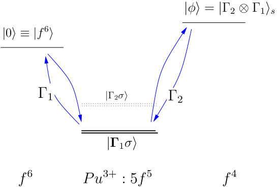
Figure 1: Virtual charge fluctuations of a model $Pu^{3+}$ ($5f^{5}$) Kramers doublet into singlet states. The addition and removal of an f-electron occur in channels $\Gamma_{1}$ and $\Gamma_{2}$ of different crystal field symmetry.

III.1 Construction of the model.

Our two-channel Kondo lattice model for heavy electron superconductivity assumes that the ground-state of an isolated magnetic ion is a Kramer’s doublet $|\Gamma_{1}\sigma\rangle$ containing an odd number $n$ of f-electrons (Fig. 1). In $PuCoGa_{5}$ and $NpPd_{5}Al_{2}$, the local moments are built out of of $f-$electrons in the $5f$ shell. The $Pu^{3+}$ ion in $PuCoGa_{5}$ is a single f-hole in a filled $j=5/2$ atomic shell, forming a $|5f^{5}\rangle$ Kramer’s doublet with $n=5$. The situation in $NpPd_{5}Al_{2}$ is more uncertain, the Curie moment extracted from the magnetic susceptibility is closest to that of a $5f^{3}$ ion with $n=3$.

We assume that the dominant spin fluctuations occur via valence fluctuations into singlet states

$$\begin{array}[]{ccccc}|0\rangle&\rightleftharpoons&|\Gamma_{1}\sigma\rangle&\rightleftharpoons&|\phi\rangle\cr f^{n+1}&&f^{n}&&f^{n-1}.\end{array}$$ (54)

To illustrate the situation, consider $PuCoGa_{5}$, where $|0\rangle\equiv|f^{6}\rangle$ is a $j=5/2$ f-shell. In a tetragonal crystal environment, the sixfold degenerate $j=5/2$ multiplet of f-electrons splits into three Kramers doublets: $\{\Gamma_{7}^{+},\ \Gamma_{7}^{-},\ \Gamma_{6}\}$. The $f^{5}$ Kramer’s doublet can be written

$$|\Gamma_{1}\sigma\rangle=f^{\dagger}_{\Gamma_{1}\sigma}|0\rangle$$ (55)

where $f^{\dagger}_{\Gamma\sigma}$ creates an f-hole in one of these three crystal field states. To form a low-energy $f^{4}$ singlet, the strong Coulomb interaction between f-electrons forces us to add a second f-hole in a different crystal field channel $\Gamma_{2}$. We assume that this state has the form

$$|\phi\rangle\equiv|\Gamma_{2}\otimes\Gamma_{1}\rangle_{s}=\frac{1}{\sqrt{2}}\sum_{\sigma=\pm 1}{\rm sgn}(\sigma)f^{\dagger}_{\Gamma_{2}\sigma}f^{\dagger}_{\Gamma_{1}\ -\sigma}|0\rangle.$$ (56)

In practice, there are many other excited states, but these are the most relevant, because they generate antiferromagnetic Kondo interactions. In a conventional Anderson model, $\Gamma_{2}$ and $\Gamma_{1}$ are the same channel. Hund’s coupling forces $\Gamma_{1}$ and $\Gamma_{2}$ to be different, and it is this physics that introduces new symmetry channels into the charge fluctuations. The simplified “atomic” model that describes this system is then

$$H_{at}=E_{0}|0\rangle\langle 0|+E_{1}|\Gamma\sigma\rangle\langle\Gamma\sigma|+E_{2}|\phi\rangle\langle\phi|$$ (57)

where $E_{1}<E_{0},E_{2}$.

In a tetragonal environment, the three Kramer’s doublets are determined by

$$f^{\dagger}_{\tilde{\Gamma}\sigma}=\sum_{m\in[-5/2,5/2]}\langle\tilde{\Gamma}\alpha|{\textstyle\frac{5}{2}}m\rangle f^{\dagger}_{m\sigma},\qquad\qquad(\sigma=\pm)$$ (58)

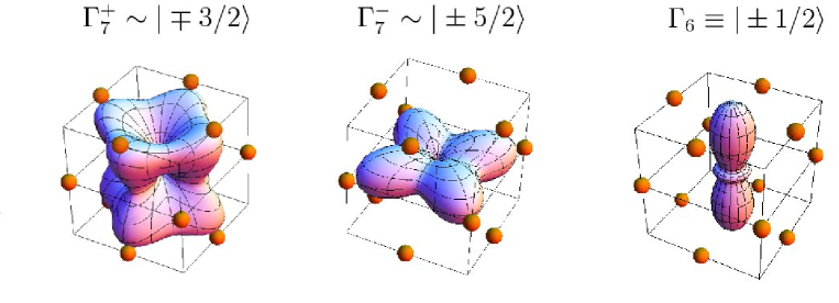
Figure 2: Showing the three crystal field states $(\Gamma_{7}^{+},\Gamma_{7}^{-},\Gamma_{6})$ with a mixing angle $\beta=\pi/10$, which maximizes the overlap of the $\Gamma_{7}^{\pm}$ with the nearby ligand atoms.$\Gamma_{7}^{+}$ overlaps with the eight out-of-plane ligand atoms, whereas $\Gamma_{7}^{-}$ overlaps strongly with the four in-plane ligand atoms. $\Gamma_{6}$ is independent of the value of $\phi$, and is always aligned along the c-axis, with minimum overlap with nearby ligand atoms.

where

$$\begin{array}[]{lccl}\Gamma_{6}:&\qquad f^{\dagger}_{\Gamma_{6}\pm}&=&f^{\dagger}_{\pm 1/2}\cr\Gamma_{7}^{+}:&\qquad f^{\dagger}_{\Gamma_{7}^{+}\pm}&=&\cos\beta f^{\dagger}_{\mp 3/2}+\sin\beta f^{\dagger}_{\pm 5/2}\cr\Gamma_{7}^{-}:&\qquad f^{\dagger}_{\Gamma_{7}^{-}\pm}&=&\sin\beta f^{\dagger}_{\mp 3/2}-\cos\beta f^{\dagger}_{\pm 5/2}.\end{array}$$ (62)

Here the mixing angle $\beta$ fine-tunes the spatial anisotropy of the $\Gamma_{7}^{\pm}$ states (see Fig. 2). Notice how the crystal mixes $\pm 5/2$ with the $\mp 3/2$ states: this is because the tetragonal crystalline environment transfers $\pm 4$ units of angular momentum to the electron. A first approximation to the crystal field states is obtained by simply setting $\beta=0$, so that $\Gamma_{7}^{+}\sim|\mp 3/2\rangle$ and $\Gamma_{7}^{-}\sim|\pm 5/2\rangle$.

When this atom is immersed into the conduction sea, the f-orbitals hybridize with conduction electrons with the same crystal symmetry. The hybridization Hamiltonian is written

$$H_{hybr}=\sum_{\sigma}\bigl{[}V_{\Gamma_{7}^{+}}\psi^{\dagger}_{\Gamma_{7}^{+}\sigma}f_{\Gamma_{7}^{+}\sigma}+V_{\Gamma_{7}^{-}}\psi^{\dagger}_{\Gamma_{7}^{-}\sigma}f_{\Gamma_{7}^{-}\sigma}+V_{\Gamma_{6}}\psi^{\dagger}_{\Gamma_{6}\sigma}f_{\Gamma_{6}\sigma}+({\rm H.c})\bigr{]}$$ (63)

where $\psi^{\dagger}_{\Gamma\sigma}$ creates a conduction electron in a Wannier state with crystal symmetry $\Gamma$ . The matrix elements of this Hamiltonian between the Kramer’s doublet and the two excited states are

$$\langle 0|H_{hyb}|\Gamma\sigma\rangle = V_{\Gamma_{1}}\psi^{\dagger}_{\Gamma_{1}\sigma}$$ (64)

$$\langle\phi|H_{hyb}|\Gamma\sigma\rangle = V_{\Gamma_{2}}\psi_{\Gamma_{2}-\sigma}\tilde{\sigma},$$ (65)

where $\tilde{\sigma}={\rm sgn}(\sigma)$. Thus the removal of an electron occurs in a different symmetry channel to the addition of an electron. The projected hybridization matrix becomes

$$H_{hybr}=\sum_{\sigma=\pm}\left(V_{\Gamma}\psi^{\dagger}_{\Gamma\sigma}|0\rangle\langle\Gamma\sigma|+\tilde{\sigma}V_{\Gamma_{2}}|\phi\rangle\langle\Gamma\sigma|\psi_{\Gamma_{2}-\sigma}+{\rm H.c}\right)$$ (66)

If we now carry out a Schrieffer Wolff transformation that integrates out the virtual charge fluctuations into the high-energy singlet states, where the energy of the absorbed, or emitted conduction electron is neglected, assuming it lies close to the Fermi energy, then we obtain

$$H_{K}=-\sum_{\sigma^{\prime},\sigma=\pm 1}\left(J_{1}|\Gamma\sigma^{\prime}\rangle\psi\phantom{{}^{\dagger}}_{\Gamma_{1}\sigma^{\prime}}\psi^{\dagger}_{\Gamma_{1}\sigma}\langle\Gamma_{1}\sigma|+J_{2}\ \tilde{\sigma}^{\prime}\psi^{\dagger}_{\Gamma_{2}-\sigma}|\Gamma_{1}\sigma^{\prime}\rangle\langle\Gamma_{1}\sigma|\psi_{\Gamma_{2}-\sigma^{\prime}}\tilde{\sigma}\right),$$ (67)

where

$$J_{1}=\frac{(V_{\Gamma_{1}})^{2}}{E_{0}-E_{1}},\qquad J_{2}=\frac{(V_{\Gamma_{2}})^{2}}{E_{2}-E_{1}},\qquad$$ (68)

This Hamiltonian can be re-written in terms of spin operators as follows

$$\hat{H}_{K}={\textstyle\frac{1}{2}}\bigl{[}J_{1}{\mbox{\boldmath$\sigma$}}^{\Gamma_{1}}(0)+J_{2}{\mbox{\boldmath$\sigma$}}^{\Gamma_{2}}(0)\bigr{]}\cdot{\mathbf{S}}_{f},$$ (69)

where we have dropped potential scattering terms and introduced the notation

$${\mathbf{S}}_{f}=\sum_{\alpha\beta}|{\Gamma_{1}}\alpha\rangle\mbox{\boldmath$\sigma$}_{\alpha\beta}\langle{\Gamma_{1}\beta}|.$$ (70)

for the spin of the Kramer’s doublet and

$${\mbox{\boldmath$\sigma$}}^{\Gamma_{1}}(0)=\psi^{\dagger}_{\Gamma_{1}\alpha}{\mbox{\boldmath$\sigma$}}_{\alpha\beta}\psi_{\Gamma_{1}\beta},\qquad{\mbox{\boldmath$\sigma$}}^{\Gamma_{2}}(0)=\psi^{\dagger}_{\Gamma_{2}\alpha}{\mbox{\boldmath$\sigma$}}_{\alpha\beta}\psi_{\Gamma_{2}\beta},$$ (71)

for the spin density at the origin in channel $\Gamma_{1}$ and channel $\Gamma_{2}$.

If we now generalize this derivation to a lattice, the interaction (69) develops at each site, producing

$$\hat{H}=\sum\limits_{{{\bf{k}}}\sigma}\epsilon_{{\bf{k}}}c_{{\bf{k}}\sigma}^{\dagger}c_{{\bf{k}}\sigma}+{\textstyle\frac{1}{2}}\sum_{j}\left[J_{1}\psi^{\dagger}_{\Gamma_{1}j\alpha}{\mbox{\boldmath$\sigma$}}_{\alpha\beta}\psi_{\Gamma_{1}j\beta}+J_{2}\psi^{\dagger}_{\Gamma_{2}j\alpha}{\mbox{\boldmath$\sigma$}}_{\alpha\beta}\psi_{\Gamma_{2}j\beta}\right]\cdot{\mathbf{S}}_{j},$$ (72)

where ${\mathbf{S}}_{j}$ is the spin operator at site $j$ and $c^{\dagger}_{{\bf{k}}\sigma}$ creates a conduction electron of momentum ${\bf{k}}$. We can relate the Wannier states at site $j$ as follows

$$\psi_{\Gamma_{1}j\alpha}=\sum_{k\sigma}[\Phi_{1{\bf{k}}}]_{\alpha\sigma}c_{{\bf{k}}\sigma}e^{i{\bf{k}}\cdot{\bf{R}}_{j}},\qquad\psi_{\Gamma_{2}j\alpha}=\sum_{k\sigma}[\Phi_{2{\bf{k}}}]_{\alpha\sigma}c_{{\bf{k}}\sigma}e^{i{\bf{k}}\cdot{\bf{R}}_{j}}$$ (73)

where

$$[\Phi_{\Gamma{\bf{k}}}]_{\alpha\sigma}=\langle k\Gamma\alpha|{\bf{k}}\sigma\rangle=\sum_{m\in[-3,3]}\langle\Gamma\alpha|3m,\frac{1}{2}\sigma\rangle Y^{3}_{m-\sigma}(\hat{{\bf{k}}})$$ (74)

is the form factor of the crystal field state. The Kondo lattice Hamiltonian then takes the form

$$\hat{H}=\sum_{{\bf{k}}\sigma}\epsilon_{{\bf{k}}}c_{{\bf{k}}\sigma}^{\dagger}c_{{\bf{k}}\sigma}+{\textstyle\frac{1}{2}}\sum_{{\bf{k}},{\bf{k}}^{\prime},j}c^{\dagger}_{{\bf{k}}\alpha}\left[J_{1}\Phi^{\dagger}_{1{\bf{k}}}\mbox{\boldmath$\sigma$}\Phi_{1{\bf{k}}^{\prime}}+J_{2}\Phi^{\dagger}_{2{\bf{k}}}\mbox{\boldmath$\sigma$}\Phi_{2{\bf{k}}^{\prime}}\right]_{\alpha\beta}c_{{\bf{k}}^{\prime}\beta}\cdot{\bf S}_{f}e^{i({\bf{k}}^{\prime}-{\bf{k}})\cdot{\bf R}_{j}}$$ (75)

For pedagogical purposes, we work largely with the model in which the matrices $\Phi_{\Gamma{\bf{k}}}=\phi_{\Gamma{\bf{k}}}{\bf 1}$ are taken to be spin-diagonal, giving rise to a simpler form

$$H=\sum_{{\bf{k}}\sigma}\epsilon_{{\bf{k}}}c_{{\bf{k}}\sigma}^{\dagger}c_{{\bf{k}}\sigma}+{\textstyle\frac{1}{2}}\sum_{{\bf{k}},{\bf{k}}^{\prime},j}J_{{\bf{k}},{\bf{k}}^{\prime}}(c^{\dagger}_{{\bf{k}}\alpha}\mbox{\boldmath$\sigma$}_{\alpha\beta}c_{{\bf{k}}^{\prime}\beta})\cdot{\bf S}_{f}e^{i({\bf{k}}^{\prime}-{\bf{k}})\cdot{\bf R}_{j}}$$ (76)

where

$$J_{{\bf{k}}{\bf{k}}^{\prime}}=J_{1}\phi_{1{\bf{k}}}\phi_{2{\bf{k}}^{\prime}}+J_{2}\phi_{2{\bf{k}}}\phi_{2{\bf{k}}^{\prime}}.$$ (77)

The results obtained using this model are easily generalized to the spin-anisotropic case by restoring the spin indices to the form factors. Lastly, we generalize our model from $SU(2)$ to symplectic-$N$ by replacing the Pauli spin operators $\mbox{\boldmath$\sigma$}_{\alpha\beta}\rightarrow({\mbox{\boldmath$\sigma$}}_{N})_{\alpha\beta}$, which we write as

$$\hat{H}=\sum\limits_{{{\bf{k}}}\sigma}\epsilon_{{\bf{k}}}c_{{\bf{k}}\sigma}^{\dagger}c_{{\bf{k}}\sigma}+{\textstyle\frac{1}{N}}\sum_{j}\left[J_{1}\psi^{\dagger}_{\Gamma_{1}j\alpha}({\mbox{\boldmath$\sigma$}_{N}})_{\alpha\beta}\psi_{\Gamma_{1}j\beta}+J_{2}\psi^{\dagger}_{\Gamma_{2}j\alpha}({\mbox{\boldmath$\sigma$}_{N}})_{\alpha\beta}\psi_{\Gamma_{2}j\beta}\right]\cdot{\mathbf{S}}_{j},$$ (78)

which in its simpler, spin-isotropic manifestation assumes the form

$$H=\sum_{{\bf{k}}\sigma}\epsilon_{{\bf{k}}}c_{{\bf{k}}\sigma}^{\dagger}c_{{\bf{k}}\sigma}+{\textstyle\frac{1}{N}}\sum_{{\bf{k}},{\bf{k}}^{\prime},j}J_{{\bf{k}},{\bf{k}}^{\prime}}c^{\dagger}_{{\bf{k}}\alpha}c_{{\bf{k}}^{\prime}\beta}S^{\beta\alpha}_{f}(j)e^{i({\bf{k}}^{\prime}-{\bf{k}})\cdot{\bf R}_{j}}$$ (79)

It is the large $N$ limit of these lattice models that we have solved in our paper.

III.2 Decoupling scheme and SU (2) symmetry

Here we detail our symplectic-$N$ decoupling scheme for the Kondo lattice. To derive the decoupling procedure, let us first focus on the interaction at a given site, temporarily suppressing site indices $j$. By applying the the dot-product relation (13 ) on the the Kondo interaction $H_{K}=\sum_{\Gamma}H_{K\Gamma}$ (69), we obtain

$$H_{K\Gamma}=\frac{J_{\Gamma}}{N}\mbox{\boldmath$\sigma$}_{N}^{\Gamma}\cdot{\bf S}_{f}=\frac{J_{\Gamma}}{N}\psi^{\dagger}_{\Gamma\alpha}\psi_{\Gamma\beta}f^{\dagger}_{\gamma}f_{\delta}(\delta_{\alpha\delta}\delta_{\beta\gamma}+\epsilon_{\alpha\gamma}\epsilon_{\delta\beta})$$ (80)

which can be rewritten in the form

$$H_{K\Gamma}=-\frac{J_{\Gamma}}{N}\sum_{\alpha\beta}\left[:(\psi^{\dagger}_{\Gamma\alpha}f_{\alpha})(f^{\dagger}_{\beta}\psi_{\Gamma\beta}):+(\psi^{\dagger}_{\Gamma\alpha}\tilde{\alpha}f^{\dagger}_{-\alpha})(\tilde{\beta}f_{-\beta}\psi_{\Gamma\beta})\right]$$ (81)

where the sum over $\alpha$ and $\beta$ runs over the $N=2k$ spin indices $\alpha,\beta\in[\pm 1,\pm k]$. (An alternative way to obtain the same result is to write the interaction as $H_{K\Gamma}=\frac{J_{\Gamma}}{2N}S_{\Gamma}^{pq}S_{f}^{qp}$ and expand the expression using (14).) When we cast this normal ordered interaction inside a path integral, we can carry out a Hubbard Stratonovich transformation on both terms, as follows:

$$H_{K\Gamma}\rightarrow\psi^{\dagger}_{\Gamma\alpha}(\bar{V}_{\Gamma}f_{\alpha}+\bar{\Delta}_{\Gamma}f^{\dagger}_{-\alpha}\tilde{\alpha})+{\rm H.c}+N\left(\frac{\bar{V}_{\Gamma}V_{\Gamma}+\bar{\Delta}_{\Gamma}\Delta_{\Gamma}}{J_{\Gamma}}\right).$$ (82)

This Hamiltonian has a local $SU(2)$ gauge invariance under the transformations

$$\left(\begin{matrix}V_{\Gamma}\cr\Delta_{\Gamma}\end{matrix}\right)\rightarrow g\left(\begin{matrix}V_{\Gamma}\cr\Delta_{\Gamma}\end{matrix}\right),\qquad\left(\begin{matrix}f_{\alpha}\cr\tilde{\alpha}f^{\dagger}_{-\alpha}\end{matrix}\right)\rightarrow g\left(\begin{matrix}f_{\alpha}\cr\tilde{\alpha}f^{\dagger}_{-\alpha}\end{matrix}\right)$$ (83)

where $g=\left({u\atop v}{v^{*}\atop-v^{*}}\right)$ is an $SU(2)$ matrix.

The exact solution of the symplectic large $N$ limit is provided by the saddle point where $V_{\Gamma}$ and $\Delta_{\Gamma}$ acquire constant expectation values. At first sight, it might be thought that the mean field erroneously predicts superconductivity under all circumstances! However, provided there is only one channel at each site, the effect of the pairing field in (82) at each site can always be absorbed by a gauge transformation in which

$$\bar{V}f_{\alpha}+\bar{\Delta}\tilde{\alpha}f_{-\alpha}^{\dagger}\rightarrow\sqrt{|V|^{2}+|\Delta|^{2}}f_{\alpha}.$$ (84)

We now restore the site label $j$ to all variables. It is convenient to recast the decoupled Hamiltonian that results in a Nambu notation, writing

$$H_{\Gamma K}=\sum_{j,\alpha>0}\left[(\tilde{\psi}^{\dagger}_{j\Gamma\alpha}{\cal V}^{\dagger}_{\Gamma j}\tilde{f}_{j\alpha})+(\tilde{f}^{\dagger}_{j\alpha}){\cal V}_{\Gamma j}\psi_{\Gamma j\alpha}\right]+\frac{N}{2J_{\Gamma}}{\rm Tr}[{\cal V}^{\dagger}_{\Gamma j}{\cal V}_{\Gamma j}]$$ (85)

where

$$\tilde{f}_{j\alpha}=\left(\begin{matrix}f_{j\alpha}\cr\tilde{\alpha}f^{\dagger}_{j-\alpha}\end{matrix}\right),\qquad\tilde{\psi}_{\Gamma j\alpha}=\left(\begin{matrix}\psi_{\Gamma j\alpha}\cr\tilde{\alpha}\psi^{\dagger}_{\Gamma j-\alpha}\end{matrix}\right)$$

are the Nambu spinors for the f-electron and conduction electron in channel $\Gamma$, while

$${\cal V}_{\Gamma j}=\left(\begin{matrix}V_{\Gamma j}&\bar{\Delta}_{\Gamma j}\cr\Delta_{\Gamma j}&-\bar{V}_{\Gamma j}\end{matrix}\right)$$

describes the Hybridization in channel $\Gamma$ at site j. The summation over $\alpha$ is restricted to positive values to avoid overcounting.

We seek uniform mean-field solutions, where ${\cal V}_{\Gamma j}$ is constant at each site. In this situation, its convenient to re-write the Wannier states and f-states in a momentum state basis,

$$\tilde{f}_{j\alpha}=\frac{1}{\sqrt{{\cal N}_{s}}}\sum_{{\bf{k}}}\tilde{f}_{{\bf{k}}\alpha}e^{i{\bf{k}}\cdot{\bf{R}}_{j}},\qquad\tilde{\psi}_{\Gamma j\alpha}=\frac{1}{\sqrt{{\cal N}_{s}}}\sum_{{\bf{k}}}\phi_{\Gamma{\bf{k}}}\tilde{c}_{{\bf{k}}\alpha}e^{i{\bf{k}}\cdot{\bf{R}}_{j}}$$

where ${\cal N}_{s}$ is the number of sites and

$$\tilde{f}_{{\bf{k}}\alpha}=\left(\begin{matrix}f_{{\bf{k}}\alpha}\cr\tilde{\alpha}f^{\dagger}_{-{\bf{k}}-\alpha}\end{matrix}\right),\qquad\tilde{c}_{{\bf{k}}\alpha}=\left(\begin{matrix}c_{{\bf{k}}\alpha}\cr\tilde{\alpha}c^{\dagger}_{-{\bf{k}}-\alpha}\end{matrix}\right).$$

Written in momentum space, the mean-field Hamiltonian is then

$$H=\sum_{{\bf{k}},\alpha>0}\left[\epsilon_{{\bf{k}}}\tilde{c}^{\dagger}_{{\bf{k}}\alpha}\tau_{3}\tilde{c}^{\dagger}_{{\bf{k}}\alpha}+\tilde{c}^{\dagger}_{{\bf{k}}\alpha}{\cal V}_{{\bf{k}}}^{\dagger}\tilde{f}_{{\bf{k}}\alpha}+\tilde{f}^{\dagger}_{{\bf{k}}\alpha}{\cal V}_{{\bf{k}}}\tilde{c}_{{\bf{k}}\alpha}+\lambda\tilde{f}_{{\bf{k}}\alpha}\tau_{3}\tilde{f}_{{\bf{k}}\alpha}\right]+N{\cal N}_{s}\left(\frac{{\rm Tr}[{\cal V}^{\dagger}_{1}{\cal V}_{1}]}{2J_{1}}+\frac{{\rm Tr}[{\cal V}^{\dagger}_{2}{\cal V}_{2}]}{2J_{2}}\right).$$ (86)

We can group these terms into a matrix that concisely describes the mean-field theory as follows

$$H=\sum_{{\bf{k}},\alpha>0}(c^{\dagger}_{{\bf{k}}\alpha},\tilde{f}^{\dagger}_{{\bf{k}}\alpha})\begin{pmatrix}\epsilon_{\bf{k}}\tau_{3}&{\cal V}_{\bf{k}}^{\dagger}\\ {\cal V}_{\bf{k}}&\lambda\tau_{3}\end{pmatrix}\left(\begin{matrix}\tilde{c}_{{\bf{k}}\alpha}\cr\tilde{f}_{{\bf{k}}\alpha}\end{matrix}\right)+N{\cal N}_{s}\left(\frac{{\rm Tr}[{\cal V}^{\dagger}_{1}{\cal V}_{1}]}{2J_{1}}+\frac{{\rm Tr}[{\cal V}^{\dagger}_{2}{\cal V}_{2}]}{2J_{2}}\right).$$ (87)

where ${\cal V}_{\bf{k}}={\cal V}_{1}\phi_{1\hat{{\bf{k}}}}+{\cal V}_{2}\phi_{2\hat{{\bf{k}}}}$. This form of the mean-field theory can be elegantly generalized to include the effects of spin-orbit coupled crystal fields by restoring the two-dimensional matrix structure to the form-factors $\Phi_{\Gamma{\bf{k}}}$,

$${\cal V}_{\bf{k}}\longrightarrow{\cal V}_{1}\Phi_{1\hat{{\bf{k}}}}+{\cal V}_{2}\Phi_{2\hat{{\bf{k}}}}$$

III.3 Mean Field Theory

To derive the mean-field theory of the uniform composite pair state CATK , we must diagonalize the mean field Hamiltonian

$$H_{{\bf{k}}}=\begin{pmatrix}\epsilon_{\bf{k}}\tau_{3}&{\cal V}_{\bf{k}}^{\dagger}\\ {\cal V}_{\bf{k}}&\lambda\tau_{3}\end{pmatrix}$$ (88)

with ${\cal V}_{{\bf{k}}}={\cal V}_{1}\Phi_{1{{\bf{k}}}}+{\cal V}_{2}\Phi_{2{{\bf{k}}}}$. A simplified treatment of the theory is obtained by assuming that $\Phi_{\Gamma{\bf{k}}}=\phi_{\Gamma{\bf{k}}}{\bf 1}$ are spin-diagonal. A more complete treatment using the general matrix form factors is given in (III.7). To examine the uniform pairing state we fix the gauge so that hybridization in channel $1$ is in the particle-hole channel, with $V_{1}=iv_{1}$, $\Delta_{1}=0$, i.e ${\cal V}_{1}=iv_{1}$ while the hybridization in channel $2$ is in the Cooper channel, $V_{2}=0$ and ${\cal V}_{2}=\Delta_{2}\tau_{2}$. The eigenvalues $\omega_{{\bf{k}}}$ of $H_{{\bf{k}}}$ are determined by

$${\rm det}(\omega\underline{1}-H_{{\bf{k}}})=\omega^{4}-2\alpha_{\bf{k}}\omega^{2}+\gamma_{\bf{k}}^{2}=0.$$

where we have introduced the notation:

$$\alpha_{\bf{k}}=v_{{\bf{k}}+}^{2}+\frac{1}{2}\left(\epsilon_{\bf{k}}^{2}+\lambda^{2}\right),\quad\gamma_{\bf{k}}^{2}=(\epsilon_{\bf{k}}\lambda-v_{{\bf{k}}-}^{2})^{2}+4(v_{1{\bf{k}}}v_{2{\bf{k}}}c_{{\bf{k}}})^{2},$$ (89)

$$v_{1{\bf{k}}}=v_{1}\phi_{1{\bf{k}}},\qquad v_{2{\bf{k}}}=\Delta_{2}\phi_{2{\bf{k}}},\qquad v_{{\bf{k}}\pm}^{2}=v_{1{\bf{k}}}^{2}\pm v_{2{\bf{k}}}^{2}.$$ (90)

The quantity $c_{{\bf{k}}}$ measures the amplitude for singlet Andreev reflection. This quantity is unity for the for the simplified spin-diagonal model. When the form factors $\Phi_{\Gamma{\bf{k}}}$ contain off-diagonal components, the above equations still hold, but with the definitions

$$\phi_{\Gamma{\bf{k}}}^{2}=\frac{1}{2}{\rm Tr}\left[\Phi^{\dagger}_{\Gamma{\bf{k}}}\Phi_{\Gamma{\bf{k}}}\right]$$

$$c_{{\bf{k}}}={\rm Tr}\left[\Phi^{\dagger}_{2{\bf{k}}}\Phi_{1{\bf{k}}}+\Phi^{\dagger}_{1{\bf{k}}}\Phi_{2{\bf{k}}}\right]/(4\phi_{1{\bf{k}}}\phi_{2{\bf{k}}})=\frac{Re{\rm Tr\left[\Phi^{\dagger}_{2{\bf{k}}}\Phi_{1{\bf{k}}}\right]}}{\sqrt{{\rm Tr}\left[\Phi^{\dagger}_{1{\bf{k}}}\Phi_{1{\bf{k}}}\right]{\rm Tr}\left[\Phi^{\dagger}_{2{\bf{k}}}\Phi_{2{\bf{k}}}\right]}}$$ (91)

The eigenvalues of $H_{{\bf{k}}}$ are given by $\omega=\omega_{{\bf{k}}\pm}$ and $\omega=-\omega_{{\bf{k}}\pm}$, where

$$\omega_{{\bf{k}}\pm}=\sqrt{\alpha_{\bf{k}}\pm(\alpha_{\bf{k}}^{2}-\gamma_{\bf{k}}^{2})^{1/2}}.$$ (92)

The quantity

$$\Delta_{{\bf{k}}}\sim v_{1{\bf{k}}}v_{2{\bf{k}}}c_{{\bf{k}}}$$

plays the role of the gap in the spectrum. Quasiparticle nodes develop on the heavy fermi surface defined by $\epsilon_{{\bf{k}}}=v^{2}_{{\bf{k}}-}/\lambda$ in directions where $\Delta_{{\bf{k}}}=0$.

The mean field equations are obtained by minimizing the free energy

$${\cal F}=-NT\sum\limits_{{\bf{k}},\pm}\log[2\cosh(\beta\omega_{{\bf{k}}\pm}/2)]+N{\cal N}_{s}\sum_{\Gamma=1,2}\frac{v_{\Gamma}^{2}}{J_{\Gamma}}$$ (93)

with respect to $\lambda$ and $(v_{\Gamma})^{2}$ ($\Gamma=1,2$), which yields

$$\begin{split}&\frac{1}{{\cal N}_{s}}\sum\limits_{{\bf{k}}\pm}\frac{\tanh(\omega_{{\bf{k}}\pm}/{2T})}{2\omega_{{\bf{k}}\pm}}\left(\lambda\pm\frac{\lambda\alpha_{\bf{k}}-\epsilon_{\bf{k}}(\epsilon_{\bf{k}}\lambda-v_{{\bf{k}}-}^{2})}{\sqrt{\alpha_{\bf{k}}^{2}-\gamma_{\bf{k}}^{2}}}\right)=0,\\ &\frac{1}{{\cal N}_{s}}\sum\limits_{{\bf{k}}\pm}\phi_{1{{\bf{k}}}}^{2}\frac{\tanh(\omega_{{\bf{k}}\pm}/{2T})}{2\omega_{{\bf{k}}\pm}}\left(2\pm\frac{(\epsilon_{\bf{k}}+\lambda)^{2}+4(v_{2{\bf{k}}}s_{{\bf{k}}})^{2}}{\sqrt{\alpha_{\bf{k}}^{2}-\gamma_{\bf{k}}^{2}}}\right)=\frac{4}{J_{1}},\\ &\frac{1}{{\cal N}_{s}}\sum\limits_{{\bf{k}}\pm}\phi_{2{{\bf{k}}}}^{2}\frac{\tanh(\omega_{{\bf{k}}\pm}/{2T})}{2\omega_{{\bf{k}}\pm}}\left(2\pm\frac{(\epsilon_{\bf{k}}-\lambda)^{2}+4(v_{1{\bf{k}}}s_{{\bf{k}}})^{2}}{\sqrt{\alpha_{\bf{k}}^{2}-\gamma_{\bf{k}}^{2}}}\right)=\frac{4}{J_{2}},\end{split}$$ (94)

where we have put $s_{{\bf{k}}}^{2}=1-c_{{\bf{k}}}^{2}$. In the normal phase either $v_{1}$ or $v_{2}$ is nonzero, corresponding to the development of the Kondo effect in the strongest channel. Therefore, there are two types of normal phase with two different Fermi surfaces:

• $J_{1}>J_{2}$, $v_{2}=0$ with spectrum

  $$\omega_{{\bf{k}}\pm}=\frac{1}{2}\left(\epsilon_{\bf{k}}+\lambda\pm\sqrt{(\epsilon_{\bf{k}}-\lambda)^{2}+4v_{1{\bf{k}}}^{2}}\right).\qquad$$ (95)

  corresponding to Kondo lattice effect in channel 1, and

• $J_{2}>J_{1}$, $v_{1}=0$, with dispersion

  $$\omega_{{\bf{k}}\pm}=\frac{1}{2}\left(\epsilon_{\bf{k}}-\lambda\pm\sqrt{(\epsilon_{\bf{k}}+\lambda)^{2}+4v_{2{\bf{k}}}^{2}}\right).\qquad$$ (96)

  corresponding to a Kondo lattice effect in channel 2.

The two normal phases are always unstable with respect to formation of the composite paired state at sufficiently low temperature.

To illustrate the method, we carried out a model calculation, in which the band structure of the conduction electrons is derived from the $3D$ tight binding model:

$$\epsilon_{\bf{k}}=-2t(\cos k_{x}+\cos k_{y}+\cos k_{z})-\mu$$ (97)

and $\mu$ is a chemical potential. Our choice of the form factors is dictated by the corresponding crystal structure of the PuCoGa₅. We take $\Phi_{1\hat{{\bf{k}}}}=\Phi_{\Gamma_{7}^{+}{\bf{k}}}$ for electrons in channel one and $\Phi_{2\hat{{\bf{k}}}}=\Phi_{\Gamma_{7}^{-}{\bf{k}}}$ for the electrons in channel two.

As we lower the temperature, the superconducting instability develops in the weaker channel. The critical temperature for the composite pairing instability is determined from equations (94) by putting $v_{2}=0^{+}$. From the third equation with logarithmic accuracy we have $\log(T_{K1}/T_{c})\simeq 1/J_{2}$ which yields

$$T_{c}\simeq\sqrt{T_{K1}T_{K2}}.$$ (98)

signaling an enhancement of superconductivity for $J_{1}\simeq J_{2}$.

It is instructive to contrast the phase diagrams of the $SU(N)$ and symplectic large $N$ limits. In the former, there is a single quantum phase transition that separates the heavy electron Fermi liquids formed via a Kondo effect about the strongest channel. In the symplectic treatment, coherence develops between the channels, immersing the two-channel quantum critical point beneath a superconducting dome. This is, to our knowledge, the first controlled mean-field theory in which the phenemenon of “avoided criticality” gives rise to superconductivity.

III.4 NMR relaxation rate

One of the precursor effects of co-operative interference between the two conduction channels appears in the NMR relaxation rate just above the transition temperature. The NMR rate is determined by

$${\cal R}\equiv\frac{1}{T_{1}T}=-\frac{I^{2}}{2\pi}\lim\limits_{\omega\to 0}\frac{\text{Im}K_{+-}^{R}(\omega)}{\omega},$$ (99)

where $I$ is the hyperfine coupling constant, $\omega$ is the NMR frequency and $K_{+-}^{R}(\omega)$ is the Fourier transform of the retarded correlation function of the electron spin densities at the nuclear site:

$$K_{+-}^{R}(\omega)=-i\int_{0}^{\infty}\langle[\hat{S}_{+}({\mathbf{0}},t),\hat{S}_{-}({\mathbf{0}},0)]\rangle e^{i\omega t}dt$$ (100)

At the mean field level, $N\to\infty$, the NMR relaxation rate follows a Korringa law.

Corrections to Korringa relaxation appear in the $1/N^{2}$ corrections to the mean field. To simplify our discussion, we assume that the Kondo exchange constants are almost degenerate $J_{1}\sim J_{2}$. In the approach to the superconducting transition, at $T>T_{c}$, in principle, we need to examine the effects of fluctuations in the hybridization and pairing amplitudes in both channel one and two. The anomalous NMR effects we are interested in come from the fluctuations in the composite pairs, and as such are driven by the interference between hybridization fluctuations in one channel and pair fluctuations in the other. To simplify our discussion we restrict our attention to the corrections induced by the interplay between fluctuations in the Kondo hybridization in channel one and pairing fluctuations in channel two. The simplified Hamiltonian for our calculation is then ${H}={H}_{c}+{H}_{0}+{H}_{2}$ with

$$\begin{split}&{H}_{0}=\sum\limits_{\mathbf{k}}\frac{2}{J_{1}}{\bar{V}}_{\mathbf{k}}\hat{V}_{\mathbf{k}}+\frac{2}{J_{2}}{\bar{\Delta}}_{\mathbf{k}}{\Delta}_{\mathbf{k}},\\ &{H}_{2}=\sum\limits_{\mathbf{k},\mathbf{q};\sigma}\left(\phi_{1\hat{\mathbf{k}}}f_{\mathbf{k}+\mathbf{q}\sigma}^{\dagger}{V}_{\mathbf{q}}c_{\mathbf{k}\sigma}+\phi_{2\hat{\mathbf{k}}}\tilde{\sigma}c_{\mathbf{k}\sigma}^{\dagger}{\Delta}_{\mathbf{q}}f_{\mathbf{q}-\mathbf{k},-\sigma}^{\dagger}+\text{H.c.}\right)\end{split}$$ (101)

and ${H}_{c}$ describes the conduction electrons. We ignore the fluctuations in the constraint fields, which do not couple to the fluctuations in $\Delta$ and $V$ in the lowest orders that we are considering. We also neglect the spin-orbit interaction effects by taking the form factors to be diagonal in spin space. Our goal is to compute the corrections to the $f$-spin correlator due to the channel interference, i.e. due to the interactions of between heavy electrons and fluctuations of slave fields described by $\hat{H}_{2}$. The interference corrections to the relaxation rate involve the product $\phi_{1\hat{{\bf{k}}}}^{*}\phi_{2\hat{{\bf{k}}}}$.

The relaxation rate will be governed by the $f$-spin correlations:

$$K_{ff}({\vec{x}};\tau)=-\langle\hat{T}_{\tau}\hat{f}_{\uparrow}^{\dagger}({\vec{x}},\tau)\hat{f}_{\downarrow}({\vec{x}},\tau)\hat{f}_{\downarrow}^{\dagger}(0,0)\hat{f}_{\uparrow}(0,0)e^{-\int\limits_{0}^{\beta}\hat{H}_{2}(\tau)d\tau}\rangle_{c},$$ (102)

where $\langle...\rangle_{c}$ denotes the connected Green’s function obtained by perturbatively expanding the time-ordered exponential in the high-temperature state where the f-electrons and conduction electrons are decoupled at the mean-field level. The leading contribution to the temperature dependence of the relaxation rate is governed by the diagram on Fig 1 which describes the effect of intersite scattering associated with an electron switching from one symmetry channel to another as it hops from site to site. To write down an analytic expression for the diagram (Fig. 1) we employ the Matsubara correlation functions for the $f-$ and $c-$ electrons together with the correlation functions of the slave fields $K_{V}({\vec{r}},\tau)=-\langle\hat{T}_{\tau}\hat{V}({\vec{r}},\tau)\hat{V}^{\dagger}(0,0)\rangle$ and $K_{\Delta}({\vec{r}},\tau)=-\langle\hat{T}_{\tau}\hat{\Delta}({\vec{r}},\tau)\hat{\Delta}^{\dagger}(0,0)\rangle$. Contrary to the situation of only one conduction channel, this contribution enhances the screening of the local spins rather then suppressing it. As in the case of the composite pair superconductivity, contribution on Fig. 1 originates from an interference between the electrons in two conduction channels undergoing a Kondo effect. To compute the relaxation rate we take into account for the onset of the Kondo screening produces renormalization of the slave boson propagators. In the Matsubara representation these propagators are:

$${\cal K}_{V}({\vec{p}};i\Omega)=\left[\frac{1}{J_{1}}+\Pi_{V}(i\Omega)\right]^{-1},\quad{\cal K}_{\Delta}({\vec{p}};i\Omega)=\left[\frac{1}{J_{2}}+\Pi_{\Delta}(i\Omega)\right]^{-1},$$ (103)

where $\Pi_{V,\Delta}(i\Omega)$ are the polarization bubbles associated with hybridization fluctuations in channel 1 and pair fluctuations in channel 2, which describe the renormalization due to the Kondo scattering. The analytic expression for the diagram on Fig.1 reads:

$$\begin{split}&\frac{T^{3}}{N^{2}}\sum\limits_{i\epsilon,i\Omega_{V},i\Omega_{\Delta}}\sum\limits_{q,p,k_{V},k_{\Delta}}G_{f}(p-k_{V})G_{f}(p+q-k_{V}){\cal K}_{V}(k_{V})\\ &\times G_{c}(p+q)G_{c}(p){\cal K}_{\Delta}(k_{\Delta})G_{f}(k_{\Delta}-p-q)G_{f}(k_{\Delta}-p),\end{split}$$ (104)

where we employed the four vector notation $p=({\vec{p}},i\omega)$ and included the form factors into the definition of the conduction electron propagators. The Matsubara frequency summations can be performed by employing the spectral function representation for the correlators in expression (104). For example,

$$G_{f,c}({\vec{p}};i\omega)=\int\limits_{-\infty}^{\infty}\frac{d\varepsilon}{\pi}\frac{\rho_{f,c}({\vec{p}},\varepsilon)}{i\omega-\varepsilon},$$ (105)

where $\rho_{f,c}({\vec{p}},\varepsilon)$ are the corresponding spectral functions. In the high temperature phase, where there is no expectation value to the hybridization $V$ or pairing field $\Delta$, the fluctuation propagators are independent of momentum $K_{V,\Delta}({\vec{p}};i\Omega)=K_{V,\Delta}(i\Omega)$. The resulting expression for the relaxation rate can be compactly written as follows

$$\frac{1}{T_{1}T}\simeq\frac{1}{N^{2}}\int\limits_{-\infty}^{\infty}W_{fc}(\omega){\cal K}_{\Delta}(\omega){\cal K}_{V}(-\omega)\frac{d\omega}{2\pi},$$ (106)

where $W_{fc}(\omega)$ is proportional to $\rho_{f}(\omega)\rho_{c}(\omega)$. The integral (106) is dominated by the frequency region near the Fermi surface. Finally, approximating the slave boson functions with ${\cal K}_{V,\Delta}(\omega)\sim J_{1,2}/\log[(T-i\omega)/T_{K}]$ hamann we obtain the following estimate for the relaxation rate

$$\frac{1}{T_{1}T}\sim\frac{1}{N^{2}}\frac{1}{\log^{2}(T/T_{K})+\pi^{2}},$$ (107)

Our result for the relaxation rate shows an upturn in $(T_{1}T)^{-1}$ with decrease in temperature, in agreement with experimental data of Curro et al. Curro2005 .

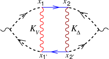
Figure 3: Channel interference contribution to the NMR relaxation rate originating from the interaction of nuclear moments with $f$-spins in the normal state. Solid lines are the conduction band propagators, wiggly lines are the propagators $K_{V}$ and $K_{\Delta}$ of the slave fields for the channel one and two correspondingly. The dashed lines are the $f$-electron propagators.

III.5 Composite pairing

Ostensibly, our mean-field theory is that of a two-band BCS superconductor, with hybridization processes that pair the heavy electrons, and Hamiltonian described by

$${\cal H}({\bf k})=\begin{pmatrix}\epsilon_{\bf{k}}\tau_{3}&{\cal V}_{\bf{k}}^{\dagger}\\ {\cal V}_{\bf{k}}&\lambda\tau_{3}\end{pmatrix}$$ (108)

However, hidden beneath the hood of theory is the underlying gauge invariance that maintains the neutrality of the f-spins. To understand the pairing, we must look not to the hybridization pairing terms, which are gauge dependent, but to gauge-invariant variables in the theory. Indeed, it is not possible to say whether the pairing is channel one, or in channel two. In the gauge we have chosen, the scattering in channel one is “normal” ${\cal V}_{1}=iv_{1}$ and pairing takes place in channel two ${\cal V}_{2}=\Delta_{2}\tau_{2}$. But suppose we make the gauge transformation (83) with $g_{j}=-i\tau_{2}$, then

$${\cal V}_{\bf k}=iv_{1{\bf k}}+v_{2{\bf k}}\tau_{2} \longrightarrow i\tau_{2}{\cal V}_{\bf k}=v_{1{\bf k}}\tau_{2}-iv_{2{\bf k}},$$ (109)

$${\bf W}=\lambda\tau_{3} \longrightarrow i\tau_{2}{\bf W}(-i\tau_{2})=-\lambda\tau_{3},$$ (111)

which transforms the Hamiltonian to one which is now pairing in channel one, and “normal” in channel two. The only gauge-invariant statement that we can make, is that superconductivity is not a product of one channel or the other, but instead derives from a coherence between the two channels.

To see this, we must combine the gauge-dependent order parameters

$${\cal V}_{1}=\left(\begin{matrix}V_{1}&\bar{\Delta}_{1}\cr\Delta_{1}&-\bar{V}_{1}\end{matrix}\right),\qquad\qquad{\cal V}_{2}=\left(\begin{matrix}V_{2}&\bar{\Delta}_{2}\cr\Delta_{2}&-\bar{V}_{2}\end{matrix}\right)$$ (112)

into the gauge-invariant composite

$${\cal V}^{\dagger}_{2}{\cal V}_{1}=\left(\begin{matrix}\bar{V}_{2}V_{1}+\bar{\Delta}_{2}\Delta_{1}&\bar{V}_{2}\bar{\Delta}_{1}-\bar{V}_{1}\bar{\Delta}_{2}\cr V_{1}\Delta_{2}-V_{2}\Delta_{1}&\bar{V}_{1}V_{2}+\bar{\Delta}_{1}\Delta_{2}\end{matrix}\right).$$

Under an $SU(2)$ gauge transformation, ${\cal V}_{1}\rightarrow g{\cal V}_{1}$, ${\cal V}_{2}^{\dagger}\rightarrow{\cal V}_{2}^{\dagger}g^{\dagger}$, so that ${\cal V}_{2}^{\dagger}{\cal V}_{1}\rightarrow{\cal V}_{2}^{\dagger}g^{\dagger}g{\cal V}_{1}={\cal V}_{2}^{\dagger}{\cal V}_{1}$ is gauge invariant. We shall now show that this matrix is equal to the amplitudes for composite pairing and hybridization, as follows:

$${\cal V}^{\dagger}_{2}{\cal V}_{1}=-\frac{J_{1}J_{2}}{N^{2}}\left[\begin{matrix}\psi^{\dagger}_{1}({\mbox{\boldmath$\sigma$}_{N}}\cdot{\bf S})\psi_{2}&\psi^{\dagger}_{1}({\mbox{\boldmath$\sigma$}}_{N}\cdot{\bf S})\epsilon\psi^{\dagger}_{2}\cr\psi_{1}\epsilon^{T}({\mbox{\boldmath$\sigma$}}_{N}\cdot{\bf S})\psi_{2}&\psi_{1}\epsilon^{T}({\mbox{\boldmath$\sigma$}}_{N}\cdot{\bf S})\epsilon\psi^{\dagger}_{2}\end{matrix}\right]$$ (113)

In the mean-field theory we have developed, ${\cal V}_{1}=iv_{1}$ and ${\cal V}_{2}=\Delta\tau_{2}$, so the composite order parameter is thus given by

$$\langle\psi^{\dagger}_{1}({\mbox{\boldmath$\sigma$}}\cdot{\bf S})\epsilon\psi^{\dagger}_{2}\rangle=-\frac{N^{2}}{J_{1}J_{2}}(iv_{1}\Delta_{2})$$ (114)

Thus it is the combination $v_{1}\Delta_{2}$ that determines the composite pairing that is ultimately manifested as resonant Andreev reflection. (see III.6)

To prove identity (113), we use a path integral approach. Here, it proves useful to employ the following matrix representation for the conduction and f-fields at each site $j$

$$F_{j}=\left(\begin{matrix}f_{j}^{T}\cr f_{j}^{\dagger}\hat{\epsilon}^{T}\end{matrix}\right)=\left(\begin{matrix}f_{j1}&f_{j-1}&\dots&f_{jk}&f_{j-k}\cr f^{\dagger}_{j-1}&-f^{\dagger}_{j1}&\dots&f^{\dagger}_{j-k}&-f^{\dagger}_{jk}\end{matrix}\right)_{j}$$ (115)

$$\Psi_{\Gamma j}=\left(\begin{matrix}\psi_{\Gamma j}^{T}\cr\psi_{\Gamma j}^{\dagger}\hat{\epsilon}^{T}\end{matrix}\right)=\left(\begin{matrix}\psi_{\Gamma j1}&\psi_{\Gamma j-1}&\dots&\psi_{\Gamma jk}&\psi_{\Gamma j-k}\cr\psi^{\dagger}_{\Gamma j-1}&-\psi^{\dagger}_{\Gamma j1}&\dots&\psi^{\dagger}_{\Gamma j-k}&-\psi^{\dagger}_{\Gamma jk}\end{matrix}\right)$$ (116)

whose columns are made up the Nambu spinors introduced in (26). Using (27), we can write $(F_{j}^{\dagger}F_{j})_{pq}=\hat{S}^{pq}(j)+\delta_{pq}$, and using (18), $\hat{S}^{pq}={{\bf S}}\cdot({\mbox{\boldmath$\sigma$}}^{T}_{N})_{pq}$, it follows that $F_{j}^{\dagger}F_{j}={{\bf S}}\cdot{\mbox{\boldmath$\sigma$}}^{T}_{N}+\underline{1}$. When we work with a path integral we shall need the normal-ordered version of this result,

$$:F_{j}^{\dagger}F_{j}:={{\bf S}}\cdot{\mbox{\boldmath$\sigma$}}^{T}_{N}$$ (117)

.

In the following derivation we temporarily suspend the site index $j$ of clarity. The notation introduced in (115) can be used to recast the hybridization terms in the interaction Hamiltonian in a more compact form as follows:

$$\sum_{\alpha>0}\tilde{\psi}_{\Gamma\alpha}{\cal V}_{\Gamma}f_{\alpha}=\frac{1}{2}\sum_{\alpha}\tilde{\psi}_{\Gamma\alpha}{\cal V}_{\Gamma}f_{\alpha}=\frac{1}{2}{\rm Tr}\left[\Psi^{\dagger}_{\Gamma}{\cal V}^{\dagger}_{\Gamma}F\right]=-\frac{1}{2}\left[F\Psi^{\dagger}_{\Gamma}{\cal V}^{\dagger}_{\Gamma}\right]=-\frac{1}{2}{\rm Tr}\left[U_{\Gamma}{\cal V}^{\dagger}_{\Gamma}\right]$$ (118)

where $U_{\Gamma}=F\Psi^{\dagger}_{\Gamma}$ is a two-dimensional matrix operator. In terms of this representation, the decoupled interaction Hamiltonian (85) at each site assumes the compact form

$$H_{K}=-\frac{1}{2}\sum_{\Gamma}\left({\rm Tr}\left[U_{\Gamma}{\cal V}^{\dagger}_{\Gamma}\right]+{\rm H.c.}\right)+\frac{N}{2J_{\Gamma}}{\rm Tr}[{\cal V}_{\Gamma}{\cal V}^{\dagger}_{\Gamma}]$$ (119)

where we have introduced the two dimensional matrices Now to evaluate the expectation value of the matrix operator ${\cal M}={\cal V}^{\dagger}_{2}{\cal V}_{1}$ we add a source term to $H_{\Gamma K}$ as follows:

$$H_{K}[\eta]=H_{K}+{\rm Tr}\left[\eta{\cal M}+(\rm H.c.)\right].$$ (120)

By varying $\eta$, we can read off the matrix $\cal M$,

$$\frac{\delta H_{\Gamma}}{\delta n_{\beta\alpha}}=({\cal M})_{\alpha\beta}$$

Now we can combine the source term in (120) with the final trace term in (119) to rewrite $H_{K}[\eta]$ in the following form

$$H_{K}[\eta]=-\frac{1}{2}\sum_{\Gamma}\left({\rm Tr}\left[U_{\Gamma}{\cal V}^{\dagger}_{\Gamma}\right]+{\rm H.c.}\right)+\frac{1}{2}{\rm Tr}\left[{\cal V}_{\Gamma}{\cal J}^{-1}_{\Gamma\Gamma^{\prime}}{\cal V}^{\dagger}_{\Gamma^{\prime}}\right]$$

where

$${\cal J}^{-1}=\left[\begin{matrix}\frac{N}{J_{1}}&2\eta\cr 2\bar{\eta}&\frac{N}{J_{2}}\end{matrix}\right]$$

If we now carry out the Gaussian integral over the ${\cal V}_{\Gamma}$, we obtain

$$H_{K}[\eta]=-\frac{1}{2}{\rm Tr}\left[U_{\Gamma}{\cal J}_{\Gamma\Gamma^{\prime}}U^{\dagger}_{\Gamma^{\prime}}\right]$$

where to leading order in $\eta$

$${\cal J}=\frac{J_{1}J_{2}}{N^{2}}\left[\begin{matrix}\frac{N}{J_{2}}&-2\eta\cr-2\bar{\eta}&\frac{N}{J_{1}}\end{matrix}\right]=\left[\begin{matrix}\frac{J_{1}}{N}&-2\frac{J_{1}J_{2}}{N^{2}}\eta\cr-2\frac{J_{1}J_{2}}{N^{2}}\bar{\eta}&\frac{J_{2}}{N}\end{matrix}\right]$$

So expanding $H_{K}[\eta]$ to leading order in $\eta$, we get

$$H_{K}[\eta]=-\frac{J_{\Gamma}}{2N}{\rm Tr}\left(U_{\Gamma}U^{\dagger}_{\Gamma}\right)+\frac{J_{1}J_{2}}{N^{2}}{\rm Tr}\left[\eta U_{2}^{\dagger}U_{1}+{\rm H.c}\right]$$

Differentiating with respect to $\eta$ then gives

$${\cal V}^{\dagger}_{2}{\cal V}_{1}\equiv\frac{J_{1}J_{2}}{N^{2}}U^{\dagger}_{2}U_{1}=\frac{J_{1}J_{2}}{N^{2}}:\left[\Psi_{2}F^{\dagger}F\Psi^{\dagger}_{1}\right]:.$$

(where the final transition from Grassman variables $U_{2}^{\dagger}U_{1}$ to operators requires the introduction of normal-ordering, denoted by colons). Using the identity (117) $:F^{\dagger}F:=\mbox{\boldmath$\sigma$}^{T}_{N}\cdot{\bf S}$, we obtain

$${\cal V}^{\dagger}_{2}{\cal V}_{1}=\frac{J_{1}J_{2}}{N^{2}}:\left[\Psi_{2}(\mbox{\boldmath$\sigma$}^{T}_{N}\cdot{\bf S})\Psi^{\dagger}_{1}\right]:=-\frac{J_{1}J_{2}}{N^{2}}:\left[\Psi_{1}^{*}(\mbox{\boldmath$\sigma$}_{N}\cdot{\bf S})\Psi^{T}_{2}\right]:$$

where we have taken the transpose of the expression in the last step. Using

$$\Psi_{1}^{*} = (\Psi_{1}^{\dagger})^{T}=\left(\dots\begin{matrix}\psi^{\dagger}_{1\alpha}\cr\tilde{\alpha}\psi_{1-\alpha}\end{matrix}\dots\right)=\left(\begin{matrix}\psi^{\dagger}_{1}\cr\psi_{1}^{T}\epsilon^{T}\end{matrix}\right),$$ (121)

$$\Psi_{2}^{T} = \left(\psi_{2},\epsilon\psi_{2}^{\dagger}\right),$$ (122)

to expand the last term, we obtain

$${\cal V}^{\dagger}_{2}{\cal V}_{1}=-\frac{J_{1}J_{2}}{N^{2}}:\left[\Psi_{1}^{*}(\mbox{\boldmath$\sigma$}_{N}\cdot{\bf S})\Psi^{T}_{2}\right]:\equiv-\frac{J_{1}J_{2}}{N^{2}}\left[\begin{matrix}\psi^{\dagger}_{1}({\mbox{\boldmath$\sigma$}_{N}}\cdot{\bf S})\psi_{2}&\psi^{\dagger}_{1}({\mbox{\boldmath$\sigma$}}_{N}\cdot{\bf S})\epsilon\psi^{\dagger}_{2}\cr\psi_{1}\epsilon^{T}(\mbox{\boldmath$\sigma$}_{N}\cdot{\bf S})\psi_{2}&\psi_{1}\epsilon^{T}({\mbox{\boldmath$\sigma$}}_{N}\cdot{\bf S})\epsilon\psi^{\dagger}_{2}\end{matrix}\right]$$ (123)

III.6 Resonant Andreev scattering

Composite pairing manifests itself through the development of an Andreev reflection component to the resonant scattering off magnetic impurities. We can capture this scattering in the mean-field theory by integrating out the f-electrons. This leads to a conduction electron Green’s function of the form

$${G}(\kappa)^{-1}=\omega-\epsilon_{\bf k}\tau_{3}-\Sigma(\kappa),$$ (124)

where $\kappa\equiv({\bf k},\omega)$ and

$$\Sigma(\kappa)={\cal V}^{\dagger}_{\bf k}(\omega-\lambda\tau_{3})^{-1}{\cal V}_{\bf k}$$ (125)

describes the resonant scattering off the quenched local moments. The hybridization matrices are written

$${\cal V}_{{\bf{k}}}={\cal V}_{1}{\hat{\Phi}}_{1{\bf{k}}}+{\cal V}_{2}{\hat{\Phi}}_{2{\bf{k}}}=iv_{1}\hat{\Phi}_{1{\bf{k}}}+\Delta\hat{\Phi}_{2{\bf{k}}}\tau_{2}$$ (126)

In our earlier discussions, the quantities $\Phi_{\Gamma{\bf{k}}}$ were assumed to be spin-diagonal. We now restore their two-dimensional matrix character, adding a carat to the symbol to denote its matrix character. These matrices act identically on particle and hole states , commuting with the isospin operators $\vec{\tau}$, but they now contain off-diagonal spin-flip terms.

It is convenient at this stage to examine the off-diagonal structure of the $\hat{\Phi}_{\Gamma{\bf{k}}}$. These two dimensional matrices are proportional to unitary matrices, and take the form

$$\hat{\Phi}_{\Gamma{\bf{k}}}=\phi_{\Gamma{\bf{k}}}{\cal U}_{\Gamma{\bf{k}}}$$

where $\phi_{\Gamma_{{\bf{k}}}}$ is a scalar and ${\cal U}_{\Gamma{\bf{k}}}$ is a two-dimensional unitary matrix. This matrix defines the interconversion between Bloch states and spin-orbit coupled Wannier states. When an electron “enters” the Kondo singlet, its spin quantization axis is rotated according to the matrix ${\cal U}_{\Gamma{\bf{k}}}$. When it leaves the ion in the same channel, this rotation process is undone, and the net hybridization matrix

$$\hat{\Phi}^{\dagger}_{\Gamma{\bf{k}}}\hat{\Phi}_{\Gamma{\bf{k}}}=(\phi_{\Gamma{\bf{k}}})^{2}\ {\bf 1}$$

is spin-diagonal. However, in the presence of composite pairing an incoming electron in channel $1$ can Andreev scatter from the ion as a hole in channel $2$. This leads to a net rotation of the spin quantization axis through an angle $\zeta_{\bf{k}}$ about an axis ${\bf n}_{{\bf{k}}}$ that both depend on the location on the Fermi surface, as follows

$$\hat{\Phi}^{\dagger}_{2{\bf{k}}}\cdot\hat{\Phi}_{1{\bf{k}}}=\phi_{2{\bf{k}}}\phi_{1{\bf{k}}}\bigl{[}c_{{\bf{k}}}+is_{{\bf{k}}}({\bf n}_{{\bf{k}}}\cdot{\mbox{\boldmath$\sigma$}})\bigr{]}$$

where $c_{{\bf{k}}}=\cos(\zeta_{\bf{k}}/2)$, $s_{{\bf{k}}}=\sin(\zeta_{{\bf{k}}}/2)$.

Armed with this information, we now continue to examine the resonant scattering off the composite-paired Kondo singlet. When we expand the self energy, we obtain a normal and Andreev component, given by

$$\Sigma(\kappa)=\Sigma_{N}(\kappa)+\Sigma_{A}(\kappa).$$ (127)

where

$$\Sigma_{N}(\kappa) = \frac{v_{1{\bf k}}^{2}}{\omega-\lambda\tau_{3}}+\frac{v_{2{\bf k}}^{2}}{\omega+\lambda\tau_{3}}$$ (128)

$$= \frac{1}{\omega^{2}-\lambda^{2}}\left[\omega(v_{1{\bf{k}}}^{2}+v_{2{\bf{k}}}^{2})+\lambda(v_{1{\bf{k}}}^{2}-v_{2{\bf{k}}}^{2})\tau_{3}\right]$$ (129)

and we denote $v_{1{\bf{k}}}=v_{1}\phi_{1{\bf{k}}},\ v_{2{\bf{k}}}=\Delta_{2}\phi_{2{\bf{k}}}$. By contrast, the Andreev terms take the form

$$\Sigma_{A}(\kappa) = \left(\frac{i\omega\tau_{2}-\lambda\tau_{1}}{(\omega^{2}-\lambda^{2})}\Phi^{\dagger}_{2{\bf{k}}}\Phi_{1{\bf{k}}}+{\rm H.c}\right)$$ (130)

$$= \frac{2v_{1{\bf{k}}}v_{2{\bf{k}}}}{(\omega^{2}-\lambda^{2})}\left[-\lambda c_{{\bf{k}}}\tau_{1}+\omega s_{{\bf{k}}}({{\bf n}_{{\bf{k}}}\cdot\mbox{\boldmath$\sigma$}})\tau_{2}\right]$$ (131)

Notice how the Andreev scattering contains two terms:

• a scalar term $\frac{2v_{1{\bf{k}}}v_{2{\bf{k}}}}{(\lambda^{2}-\omega^{2})}\lambda c_{{\bf{k}}}\tau_{1}$ that is finite at the Fermi energy ($\omega=0$), with gap symmetry of the form

  $$\Delta_{{\bf{k}}}\propto{\rm Tr\Phi^{\dagger}_{2{\bf{k}}}\Phi_{1{\bf{k}}}}\sim\phi_{1{\bf{k}}}\phi_{2{\bf{k}}}c_{{\bf{k}}}$$

• a “triplet” term $-\omega\frac{2v_{1{\bf{k}}}v_{2{\bf{k}}}}{(\lambda^{2}-\omega^{2})}\left[s_{{\bf{k}}}({{\bf n}_{{\bf{k}}}\cdot\mbox{\boldmath$\sigma$}})\tau_{2}\right]$ which is odd in frequency and vanishes on the Fermi surface.

In practice, the nodes of the pair wavefunction are dominated by the symmetry of the function $c_{{\bf{k}}}$. When an electron Andreev reflects through one hybridization channel into the other, it acquires orbital angular momentum. For example, the “up” states of the $\Gamma_{7}^{+}\sim|-3/2\rangle$ and $\Gamma_{7}^{-}\sim|+5/2\rangle$ differ by $l=4$ units of angular momentum, so the resulting gap has the symmetry of an $l=4$ spherical harmonic, or $g-$ wave symmetry. By contrast, the up states of the $\Gamma_{7}^{+}\sim|-3/2\rangle$ and $\Gamma_{6}\sim|+1/2\rangle$ differ by $l=2$ units of angular momentum, and the resulting gap has the symmetry of an $l=2$ spherical harmonic, or $d$- wave symmetry, as shown below:

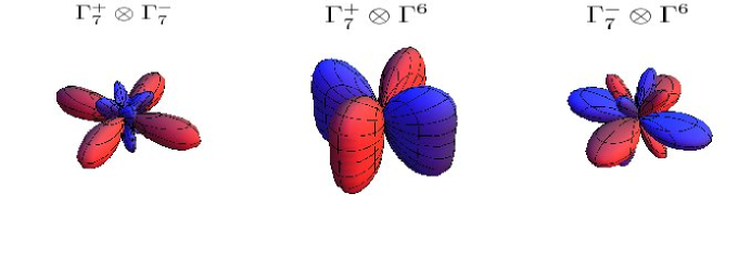
Figure 4: Showing the three possible gap functions: $\Gamma^{+}_{7}\otimes\Gamma^{-}_{7}$, $\Gamma^{+}_{7}\otimes\Gamma_{6}$, and $\Gamma_{7}^{-}\otimes\Gamma_{6}$ for mixing angle $\beta=\pi/10$. Positive nodes are colored red, while negative nodes are blue. $\Gamma^{+}_{7}\otimes\Gamma^{-}_{7}$ is g-wave(l = 4), while $\Gamma^{\pm}_{7}\otimes\Gamma_{6}$ are both d-wave(l=2).

III.7 Dispersion in the presence of strong spin-orbit coupling

To develop a mean-field theory in the presence of spin-orbit scattering, we need to diagonalize the the conduction electron Green’s function. The eigenvalues are determined by the condition

$${\rm det}[\omega\underline{1}-{\cal H}({\bf{k}})]=0$$

If we integrate out the f-electrons, this becomes this becomes

$${\rm det}[\omega\underline{1}-{\cal H}({\bf{k}})]=(\omega^{2}-\lambda^{2})^{2}{\rm det}[{\cal G}(\kappa)^{-1}]=(\omega^{2}-\lambda^{2})^{2}{\rm det}[\omega-\epsilon_{{\bf{k}}}\tau_{3}-\Sigma(\kappa)]$$

Now since $\Sigma(\kappa)\propto\frac{1}{\omega^{2}-\lambda^{2}}$, it is convenient to factor this term out of the determinant, so that

$${\rm det}[\omega\underline{1}-{\cal H}({\bf{k}})]=(\omega^{2}-\lambda^{2})^{-2}{\rm det}[(\omega^{2}-\lambda^{2}){\cal G}(\kappa)^{-1}]$$

Now

$$(\omega^{2}-\lambda^{2}){\cal G}(\kappa)^{-1}=\omega(A+D(\mbox{\boldmath$\sigma$}\cdot{\bf n}_{{\bf{k}}})\tau_{2})-B\tau_{3}+C\tau_{1}$$ (132)

where

$$A = \omega^{2}-\lambda^{2}-v_{{\bf{k}}+}^{2}$$ (133)

$$B = \epsilon_{{\bf{k}}}(\omega^{2}-\lambda^{2})+\lambda v_{{\bf{k}}-}^{2}$$ (134)

$$C = 2\lambda v_{1{\bf{k}}}v_{2{\bf{k}}}c_{{\bf{k}}}$$ (135)

$$D = 2v_{1{\bf{k}}}v_{2{\bf{k}}}s_{{\bf{k}}}$$ (136)

and $v_{{\bf{k}}\pm}^{2}=v_{1{\bf{k}}}^{2}\pm v_{2{\bf{k}}}^{2}$.

Now if we project the Hamiltonian into states where $(\bf n_{{\bf{k}}}\cdot\mbox{\boldmath$\sigma$})=\pm 1$, we can replace $A+D(\mbox{\boldmath$\sigma$}\cdot{\bf n}_{{\bf{k}}})\tau_{2}\rightarrow A\pm D\tau_{2}$, i.e

$${\rm det}[\omega\underline{1}-{\cal H}({\bf{k}})] = \prod_{\pm}\frac{{\rm det}[\omega(A\pm D\tau_{2})-B\tau_{3}+C\tau_{1}]}{(\omega^{2}-\lambda^{2})}$$ (137)

The presence of the $\omega^{2}-\lambda^{2}$ terms in the denominator results from integrating out the f-electrons. In actual fact, there are no zeroes of the determinant at $\omega=\pm\lambda$, and the the $\omega^{2}-\lambda^{2}$ denominators in these expressions act to factor out the false zeros $\omega=\pm\lambda$ in the numerator that have been introduced by integrating out the f-electrons. If now expand the numerator:

$${\rm det}[\omega(A\pm D\tau_{2})-B\tau_{3}+C\tau_{1}] = [\omega^{2}A^{2}-\omega^{2}D^{2}-B^{2}-C^{2}]$$ (138)

$$=\omega^{2}\left[(\omega^{2}-\lambda^{2}-v_{+}^{2})^{2}-(2v_{1{\bf{k}}}v_{2{\bf{k}}}s_{{\bf{k}}})^{2}\right] - \left[\epsilon_{{\bf{k}}}(\omega^{2}-\lambda^{2})+\lambda v_{-}^{2}\right]^{2}-\left[2\lambda v_{1{\bf{k}}}v_{2{\bf{k}}}c_{{\bf{k}}}\right]^{2}.$$ (139)

Notice that we get the same result for both $\pm D$. Now we know that there is a factor $(\omega^{2}-\lambda^{2})$ in this expression, so we can write

$${\rm det}[\omega(A\pm D\tau_{2})-B\tau_{3}+C\tau_{1}] = (\omega^{2}-\lambda^{2})\left[\omega^{4}-2\omega^{2}\alpha_{{\bf{k}}}+\gamma^{2}_{{\bf{k}}}\right]$$ (140)

By a direct expansion of this expression and a comparison of terms with (138), we are able to confirm that this factorization works, with

$$\alpha_{{\bf{k}}} = v_{{\bf{k}}+}^{2}+\frac{1}{2}(\lambda^{2}+\epsilon_{{\bf{k}}}^{2})$$ (141)

$$\gamma^{2}_{{\bf{k}}} = (\epsilon_{{\bf{k}}}\lambda-v_{{\bf{k}}-}^{2})^{2}+(2v_{1{\bf{k}}}v_{2{\bf{k}}}c_{{\bf{k}}})^{2}$$ (142)

Thus

$${\rm det}[\omega\underline{1}-{\cal H}({\bf{k}})]=\left[\omega^{4}-2\omega^{2}\alpha_{{\bf{k}}}+\gamma^{2}_{{\bf{k}}}\right]^{2}$$ (143)

The surviving yet crucial effect of the spin-flip scattering is entirely contained in the $c_{{\bf{k}}}$ factor in $\gamma_{{\bf{k}}}$. The Boguilubov quasiparticles in the composite paired state preserve their Kramer’s degeneracy, with dispersion given by

$$\omega_{{\bf{k}}\pm}=\sqrt{\alpha_{\bf{k}}\pm(\alpha_{\bf{k}}^{2}-\gamma_{\bf{k}}^{2})^{1/2}},$$

as described in section (III.3).

III.8 Crystal Fields determine the gap symmetry.

Here we calculate the form factors for the two-channel Kondo model in a tetragonal crystal field environment. In a tetragonal crystal field environment, the Kramer’s doublets are given by $|\Gamma\pm\rangle=|jm\rangle\langle jm|\Gamma\pm\rangle$, ($j=5/2$), where from (62)

$$\begin{array}[]{lccl}\Gamma_{6}:&\qquad f^{\dagger}_{\Gamma_{6}\pm}&=&|{\pm 1/2}\rangle\cr\Gamma_{7}^{+}:&\qquad f^{\dagger}_{\Gamma_{7}^{+}\pm}&=&\cos\beta|{\mp 3/2}\rangle+\sin\beta|{\pm 5/2}\rangle\cr\Gamma_{7}^{-}:&\qquad f^{\dagger}_{\Gamma_{7}^{-}\pm}&=&\sin\beta|{\mp 3/2}\rangle-\cos\beta|{\pm 5/2}\rangle\end{array}$$ (147)

The matrices representing these crystal field states are then

$${\textstyle\ m:\ \frac{5}{2}\ \qquad\ \ \hskip 2.168pt-\frac{5}{2}}\ \ \hskip 10.84006pt\alpha:$$ (148)

$$\langle\Gamma_{6}\alpha|jm\rangle = \ \ \ \ \hskip 2.168pt\left(\begin{matrix}0&0&1&0&0&0\cr 0&0&0&1&0&0\end{matrix}\right),\begin{matrix}+\cr-\end{matrix}$$ (149)

$$\langle\Gamma_{7^{+}}\alpha|jm\rangle = \left(\begin{matrix}\sin(\beta)&0&\ \ 0&\ \ 0&\cos(\beta)&0\cr 0&\cos(\beta)&\ \ 0&\ \ 0&0&\sin(\beta)\end{matrix}\right),$$ (150)

$$\langle\Gamma_{7^{-}}\alpha|jm\rangle = \left(\begin{matrix}-\cos(\beta)&0&\ \ 0&\ \ 0&\sin(\beta)&0\cr 0&\sin(\beta)&\ \ 0&\ \ 0&0&\cos(\beta)\end{matrix}\right).$$ (151)

while the overlap of the Bloch states with the spin-orbit coupled Wannier states $|jm\rangle$ ($j=5/2$, $m\in[-j,j]$) is given by

$$\langle jm|{\bf{k}}\sigma\rangle=\sigma\sqrt{\frac{\frac{7}{2}-m\sigma}{7}}Y^{3}_{m-\frac{1}{2}\sigma}(\hat{\bf{k}})=\left(\begin{matrix}\sqrt{\frac{1}{7}}Y^{3}_{2}({\bf{k}})&-\sqrt{\frac{6}{7}}Y^{3}_{3}({\bf{k}})\cr\vdots&\vdots\cr\sqrt{\frac{6}{7}}Y^{3}_{-3}({\bf{k}})&-\sqrt{\frac{1}{7}}Y^{3}_{-2}({\bf{k}})\end{matrix}\right).$$ (152)

where we have used the Clebsch Gordon coefficient $\langle jm|lm-\frac{1}{2}\sigma,\frac{1}{2}\ \frac{1}{2}\sigma\rangle=\sigma\sqrt{\frac{\frac{7}{2}-m\sigma}{7}}$, ($\sigma=\pm 1$). We obtain the form factors of the Wannier states by multiplying matrices from (148) with the matrix elements (148):

$$[\Phi_{\Gamma{\bf{k}}}]_{\alpha\sigma}=\sum_{m}\langle\Gamma\alpha|jm\rangle\langle jm|{\bf{k}}\sigma\rangle$$ (153)

The form factors are then given by

$$\Phi_{\Gamma_{7}^{+}{\bf{k}}}=\frac{1}{\sqrt{7}}\left[\begin{matrix}{\sqrt{5}cY^{3}_{-2}(\hat{\bf{k}})+sY^{3}_{2}(\hat{\bf{k}})}&-\sqrt{6}sY^{3}_{3}(\hat{\bf{k}})-\sqrt{2}cY^{3}_{-1}(\hat{\bf{k}})\cr\sqrt{6}sY^{3}_{-3}(\hat{\bf{k}})+\sqrt{2}cY^{3}_{1}(\hat{\bf{k}})&\ -\sqrt{5}cY^{3}_{2}(\hat{\bf{k}})-sY^{3}_{-2}(\hat{\bf{k}})\end{matrix}\right],$$ (154)

$$\Phi_{\Gamma_{7}^{-}{\bf{k}}}=\frac{1}{\sqrt{7}}\left[\begin{matrix}{\sqrt{5}sY^{3}_{-2}(\hat{\bf{k}})-cY^{3}_{2}(\hat{\bf{k}})}&\sqrt{6}cY^{3}_{3}(\hat{\bf{k}})-\sqrt{2}sY^{3}_{-1}(\hat{\bf{k}})\cr-\sqrt{6}cY^{3}_{-3}(\hat{\bf{k}})+\sqrt{2}sY^{3}_{1}(\hat{\bf{k}}\ )&\ -\sqrt{5}sY^{3}_{2}(\hat{\bf{k}})+cY^{3}_{-2}(\hat{\bf{k}})\end{matrix}\right]$$ (155)

$$\Phi_{\Gamma_{6}{\bf{k}}}=\frac{1}{\sqrt{7}}\left[\begin{matrix}\sqrt{3}Y^{3}_{0}(\hat{\bf{k}})&-\sqrt{4}Y^{3}_{1}(\hat{\bf{k}})\cr\sqrt{4}Y^{3}_{-1}(\hat{\bf{k}})&-\sqrt{3}Y^{3}_{0}(\hat{\bf{k}})\end{matrix}\right]$$

where we use the shorthand $c\equiv\cos(\beta)$, $s\equiv\sin(\beta)$ to denote the cosine and sine of the mixing angle. Each of these functions is time-reversal invariant, namely they satisfy

$$\epsilon(\Phi^{\dagger}_{\Gamma-{\bf{k}}})^{T}\epsilon^{T}=\Phi_{\Gamma{\bf{k}}}$$

There are basically two symmetry classes of superconductor that are possible in our model, one formed from $\Gamma_{7}\otimes\Gamma_{6}$, the other formed from $\Gamma_{7}^{+}\otimes\Gamma_{7}^{-}$ (Fig. 4). The latter is argued to be preferably, because it is these two states that have the maximum overlap with nearby ligand atoms. The form factors $\phi_{\Gamma{\bf{k}}}$ are determined from

$$(\phi_{1{\bf{k}}})^{2} = \frac{1}{2}{\rm Tr}[\Phi^{\dagger}_{1{\bf{k}}}\Phi_{1{\bf{k}}}]$$ (156)

$$(\phi_{2{\bf{k}}})^{2} = \frac{1}{2}{\rm Tr}[\Phi^{\dagger}_{2{\bf{k}}}\Phi_{2{\bf{k}}}]$$ (157)

For general $\beta$ , these are form-factors with point nodes along the c-axis, but no lines of nodes. The gap function is however determined from the symmetry of

$$\phi_{1{\bf{k}}}\phi_{2{\bf{k}}}c_{{\bf{k}}}=\frac{v_{1}\Delta_{2}}{4}{\rm Tr}[\Phi^{\dagger}_{2{\bf{k}}}\Phi_{1{\bf{k}}}+{\rm H.c.}]$$

In our model, we have chosen $\Gamma_{1}\equiv\Gamma_{7}^{+}$ corresponding to the out-of-plane ligand atoms and $\Gamma_{2}\equiv\Gamma_{7}^{-}$ corresponding to the in-plane ligand atoms. In this case, when we expand this function in detail, we find it has the form

$$\phi_{1{\bf{k}}}\phi_{2{\bf{k}}}c_{{\bf{k}}}=\cos(2\beta)\Delta_{g1}({\bf{k}})-\sin(2\beta)\Delta_{g2}({\bf{k}})$$

where $\Delta_{g1}$ and $\Delta_{g2}$ are g-wave gap functions of the form

$$\Delta_{g1}({\bf{k}})=\frac{\sqrt{5}}{16\pi}\cos(4\phi)\sin^{2}[\theta]$$

and

$$\Delta_{g2}({\bf{k}})=\frac{3}{16\pi}\sin^{2}(\theta)(3+\cos(2\theta)).$$

For small $\beta$, the gap is dominated by $\Delta_{g1}({\bf{k}})$

IV Frustrated Magnetism

As a test of symplectic-$N$, we would like to return to the origins of $SP(N)$, initially developed to treat antiferromagnetism on frustrated latticesreadsachdev91 . $SP(N)$ describes antiferromagnetism, or the formation of valence bonds well, but cannot handle ferromagnetism, the fluctuations of those bonds. This weakness can already be seen in the simplest model in frustrated magnetism, the $J_{1}-J_{2}$ Heisenberg model on a square lattice doucot

$$H=J_{1}\sum_{{\bf{x}},\mu}\vec{S}_{\bf{x}}\cdot\vec{S}_{{\bf{x}}+\mu}+J_{2}\sum_{{\bf{x}},\mu^{\prime}}\quad\vec{S}_{{\bf{x}}}\cdot\vec{S}_{{\bf{x}}+\mu^{\prime}},$$ (158)

where $J_{1}$ and $J_{2}$ are the first and next nearest neigbor couplings.

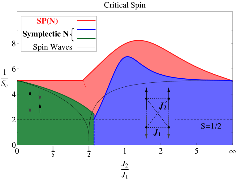
Figure 5: The $J_{1}-J_{2}$ Heisenberg model: We compare the critical spin $S_{c}=\left(\frac{n_{b}}{N}\right)_{c}$, below which there is no long range order in the ground state, calculated within $SP(N)$ (bold red line), symplectic-$N$ (blue and green lines), and spin wave theorychandradoucot (thin black line). $J_{1}$ and $J_{2}$ are nearest and next nearest neighbor antiferromagnetic bonds, as shown in the figure. For small $J_{2}/J_{1}$, the spins configurations are staggered, while for large $J_{2}/J_{1}$, the ground state breaks lattice symmetry to develop collinear order as shown in the figure. $SP(N)$ (bold red line) tends to overstabilize the long range ordered phases, most dramatically on the one sublattice side, where the critical spin is independent of the strength $J_{2}$ of the frustrating diagonal bondsoleg . Symplectic-$N$ restores the frustration-induced fluctuations by treating both ferromagnetic and antiferromagnetic bonds, on equal footing, which corrects this overstabilization.

For large $J_{1}/J_{2}$, the ground state is the typical Néel state, where diagonal spins are ferromagnetically aligned(see Fig 5 inset). As $J_{2}$ increases, these diagonal bonds become increasingly frustrated, destabilizing the long range order, which requires higher and higher spin, $S_{c}$ for magnetic order.

At large $J_{2}/J_{1}$, this model describes two interpenetrating Néel lattices that are classically decoupled. When fluctuations are included, a biquadratic interaction locks the two sublattices together in a collinear configurationccl (see Fig 5). The nearest neighbor bond, $J_{1}$, initially stabilizes the collinear state, but, as the frustration increases, the long range order is eventually destabilized.

In quantum magnetism, one generally uses a Schwinger boson spin representation. The $SP(N)$ approach introduced by Read and Sachdev readsachdev91long decouples the antiferromagnetic interaction in the following manner

$$H_{I}=-\frac{J}{N}B^{\dagger}_{12}B_{12}\quad\qquad\qquad\qquad\qquad\qquad\qquad SP(N).$$

where $B^{\dagger}_{21}=\sum_{\sigma}\tilde{\sigma}b^{\dagger}_{2\sigma}b^{\dagger}_{1-\sigma}$ creates a valence bond $(2,1)$ between sites one and two. The $SP(N)$ approach captures the competition between first and next nearest neighbor links for valence bondsoleg , but misses the frustrating effect of the ferromagnetic bonds, resulting in overstabilization of the collinear statereadsachdev91long . If we decompose $H_{I}$ in terms of spin generators, we find it contains a mix of “spins” and “dipoles”

$$H_{I}=\frac{J}{2N}(\vec{S}_{1}\cdot\vec{S}_{2}-{\vec{\cal P}}_{1}\cdot{\vec{\cal P}}_{2}),\quad\qquad\qquad\qquad\underline{SP(N)}.$$ (159)

This inadvertent inclusion of dipoles with a negative, i.e ferromagnetic sign, tends to cancelling out the frustrating effect of ferromagnetic bonds. For instance, in the $J_{1}-J_{2}$ model, the critical spin for developing long-range antiferromagnetism is artificially independent of the frustration in the the $SP(N)$ mean-field theoryoleg (Fig. 5.).

In the symplectic- $N$ approach, we decouple the interaction exclusively in terms of the generators of $SP(N)$ $S_{\alpha\beta}=b^{\dagger}_{\alpha}b_{\beta}-\tilde{\alpha}\tilde{\beta}b^{\dagger}_{-\beta}b_{\alpha}$. Using the explicit form of the symplectic spins, we find the Heisenberg interaction decouples into two terms

$$H_{I}=\frac{J}{N}\vec{S}_{1}\cdot\vec{S}_{2}=-\frac{J}{N}\left[B^{\dagger}_{21}B_{21}-A^{\dagger}_{21}A_{21}\right],\qquad\qquad{\hbox{\text@underline{Symplectic $N$.}}}$$ (160)

where $A_{21}=\sum_{\sigma}b^{\dagger}_{2\sigma}b_{1\sigma}$. The second term in this interaction describes ferromagnetic correlations, which were absent in the original applications. The operators $A_{21}$ and $A^{\dagger}_{21}$ “resonate” a valence bond linked to a third site, between sites one and two: $(1,3)\rightleftharpoons(2,3)$. When the bond resonates between sites 1 and 2, the amplitude for singlets to form between the two sites is reduced, giving rise to a ferromagnetic correlation between sites 1 and 2. The exclusion of dipole spins requires that we treat these two terms in equal measure.

When we carry out a Hubbard Stratonovich factorization of the Heisenberg interaction (160), it separates into two amplitudes $h$ and $\Delta$ describing bond resonance and condensation respectively

$$J\vec{S}_{1}\cdot\vec{S}_{2}=\left(b^{\dagger}_{2\sigma},\tilde{\sigma}b_{2\ -\sigma}\right)\left[\begin{matrix}h&\Delta\cr\bar{\Delta}&\bar{h}\end{matrix}\right]\left(\begin{matrix}b_{1\sigma}\cr\tilde{\sigma}b^{\dagger}_{1\ -\sigma}\end{matrix}\right)+\frac{N}{J}(|\Delta|^{2}-|h|^{2}).$$ (161)

This kind of decoupling scheme was first proposed by Ceccatto, Gazza and Trumperceccatto for $SU(2)$ spins, where it is one of many alternative decoupling procedures. In symplectic-$N$, it is the unique form preserving the time reversal parity of the spins. Now we would like to see if and when the ferromagnetic $h$ bonds develop and what effect they have on the physics. To do this we examine the action,

$$N{\cal S}[b,\Delta,h,\lambda]=\int_{0}^{\beta}d\tau\sum_{i}[\sum_{\sigma}b^{\dagger}_{i\sigma}(\partial_{\tau}-\lambda_{i})b_{i\sigma}+\lambda_{i}NS]+\sum_{(ij)}J_{ij}\vec{S}_{i}\cdot\vec{S}_{j}$$ (162)

with $J_{ij}\vec{S}_{i}\cdot\vec{S}_{j}$ given above. We assume all bond fields are uniform and static, depending only on $i-j$. The constraint, $n_{b}=NS$ is enforced by the Lagrange multiplier $\lambda_{i}$. As the action is quadratic in the Schwinger bosons, they can easily be integrated out to find the mean field Free energy:

$$\frac{F_{MF}}{N\mathcal{N}}=\frac{1}{\mathcal{N}}\sum_{k}\log[2\sinh\frac{\beta\omega_{k}}{2}]+\frac{1}{\mathcal{N}}\sum_{(i,j)}\frac{\bar{\Delta}_{ij}\Delta_{ij}-\bar{h}_{ij}h_{ij}}{J_{ij}}-\lambda(2S+1)$$ (163)

where $(i,j)$ is a pair of sites with nonzero $J_{ij}$, $\mathcal{N}$ is the number of sites, $\omega_{k}=\sqrt{|\lambda-h_{k}|^{2}-|\Delta_{k}|^{2}}$, and $h_{k}$ and $\Delta_{k}$ are the Fourier transforms of $h_{ij}$ and $\Delta_{ij}$. The Néel state is described by $\Delta$’s along the nearest neighbor bonds, and induced $h_{d}$ along the diagonal bonds for finite $J_{2}$.

$$\omega_{k}^{Neel}=\sqrt{(\lambda+4h_{d}c_{x}c_{y})^{2}-4\Delta^{2}(s_{x}+s_{y})^{2})},$$ (164)

where $c_{l}=\cos k_{l}a$ and $s_{l}=\sin k_{l}a$. For large $J_{2}$, the classical decoupled state consists of $\Delta_{d}$ along the diagonal bonds, where the magnitude of $\Delta_{d}$ is the same on both sublattices, but the phase between the two is free. When fluctuations are introduced, the lattice symmetry is broken by the collinear order; we choose the phase so the collinear state is antiferromagnetic along $\hat{y}$($\Delta_{y}$), which induces ferromagnetism along $\hat{x}$($h_{x}$), giving the dispersion,

$$\omega_{k}^{Ising}=\sqrt{(\lambda+2h_{x}c_{x})^{2}-(4\Delta_{d}c_{x}s_{y}+2\Delta_{y}s_{y})^{2})}$$ (165)

The values of $h$, $\Delta$, and $\lambda$ are chosen to minimize the Free energy using the mean field equations: $\partial F/\partial\lambda=0$, $\partial F/\partial h=0$ and $\partial F/\partial\Delta=0$, for all $h$’s and $\Delta$’s in the particular problem. $SP(N)$ proceeds similarly except that the $h$’s are fixed to be zero.

We are interested in the zero temperature case, where in two dimensions, the Schwinger bosons can condense when the gap in the spectrum vanishes, signaling the onset of long range magnetic order. As we are primarily interested in the spin above which the system orders magnetically, $S_{c}$, we only consider the unpopulated condensate.

The minimum gap in the spectrum is fixed at $(\pm\pi/2,\pm\pi/2)$ and $(0,\pm\pi/2)$ for the Néel and Ising states, respectively. Setting that gap to zero gives us an algebraic relation between the parameters supplementing the mean field equations. After the parameters are determined from $\partial F/\partial h$ and $\partial F/\partial\Delta$, $\partial F/\partial\lambda=0$ can be used to find the critical spin,

$$S_{c}+\frac{1}{2}=\frac{1}{2}\int_{k}\frac{\lambda+2h_{k}}{\omega_{k}}.$$ (166)

Results from these calculations for both symplectic-$N$ and $SP(N)$ are shown in Fig LABEL:Sc, along with a comparision to spin wave theory. $SP(N)$ drastically overestimates the stability of the ordered states, which is corrected by the ferromagnetic bonds included in symplectic-$N$. For both large $N$ theories, the regions of Néel and Ising order overlap, indicating a first order transition, while spin wave theory predicts a second order transition for all $S$, with an intervening region of spin liquid. However, when higher order corrections are taken into account, modified spin wave theory gives exactly the results of symplectic-$N$wu .

We can draw an analogy between frustrated magnetism and heavy fermion superconductivity, in which previous large $N$ techniques were able to treat only one of two possible phenomena, ferromagnetism and antiferromagnetism in the case of frustrated magnetism, Fermi liquid physics and superconductivity in heavy fermion superconductors. In both situations, symplectic-$N$ enables simultaneous and equivalent treatment of both phenomena and significantly improves upon the previous results.

References

- (1) A.A. Abrikosov, Physics(Long Island City, NY) 2, 5 (1965).
- (2) I. Affleck, Z. Zou, T. Hsu and P. W. Anderson, Phys. Rev. B 38, 745, (1988).
- (3) D.P. Arovas and A. Auerbach Phys. Rev. B, 38, 316 (1988).
- (4) P. Coleman, A. M. Tsvelik, N. Andrei and H. Y. Kee, Phys. Rev. B 60, 3608 (1999).
- (5) N. J. Curro et al., Nature (London) 434, 622 (2005).
- (6) N. Read and Subir Sachdev, Phys. Rev. Lett. 66, 1773 (1991);
- (7) P. Chandra and B. Doucot, Phys. Rev. B 38, 9335 (1988).
- (8) P. Chandra and B. Doucot, Phys. Rev. B38, 9335, 1988
- (9) P. Chandra, P. Coleman and A. I. Larkin, Phys. Rev. Lett. 64, 88 (1990).
- (10) O. Tchenyshyov, R. Moessner and S. L. Sondhi, Europhysics Letters 73, 278-284 (2006).
- (11) D. R. Hamann, Phys. Rev. 158, 570 (1967).
- (12) N. Read and Subir Sachdev, Int. Jour. of Mod. Phys. B 5, 219(1991).
- (13) H.A. Ceccatto, C.J. Gazza and A.E. Trumper, Phys. Rev. B 47, 12329 - 12332 (1993).
- (14) C. Wu and S. Zhang, Phys. Rev. B 71, 155115 (2005).