The Plasma Structure of the Cygnus Loop from the Northeastern Rim to the Southwestern Rim

Abstract

The Cygnus Loop was observed from the northeast to the southwest with XMM-Newton. We divided the observed region into two parts, the north path and the south path, and studied the X-ray spectra along two paths. The spectra can be well fitted either by a one-component non-equilibrium ionization (NEI) model or by a two-component NEI model. The rim regions can be well fitted by a one-component model with relatively low $kT_{\rm e}$ whose metal abundances are sub-solar (0.1–0.2). The major part of the paths requires a two-component model. Due to projection effects, we concluded that the low $kT_{\rm e}$ ($\sim$0.2 keV) component surrounds the high $kT_{\rm e}$ ($\sim$0.6 keV) component, with the latter having relatively high metal abundances ($\sim$5 times solar). Since the Cygnus Loop is thought to originate in a cavity explosion, the low $kT_{\rm e}$ component originates from the cavity wall while the high $kT_{\rm e}$ component originates from the ejecta.

The flux of the cavity wall component shows a large variation along our path. We found it to be very thin in the south-west region, suggesting a blowout along our line of sight. The metal distribution inside the ejecta shows non-uniformity, depending on the element. O, Ne and Mg are relatively more abundant in the outer region while Si, S and Fe are concentrated in the inner region, with all metals showing strong asymmetry. This observational evidence implies an asymmetric explosion of the progenitor star. The abundance of the ejecta also indicates the progenitor star to be about 15 $\rm\,M_{\odot}$.

1 Introduction

A supernova remnant (SNR) reflects the abundance of the progenitor star when the remnant is young and that of the interstellar matter (ISM) when it becomes old. In this way, we can study the evolution of the ejecta and the ISM. The Cygnus Loop is a proto-typical middle-aged shell-like SNR. The angular diameter is about 2^∘.4 and it is very close to us (540 pc; Blair et al. 2005), implying a diameter of $\sim$23 pc. The estimated age is about 10000 years, less than half that based on the previous distance estimate of 770 pc Minkowski (1958).

Since the Cygnus Loop is an evolved SNR, the bright shell mainly consists of a shock-heated surrounding material. Its supernova (SN) explosion is generally considered to have occurred in a preexisting cavity McCray & Snow (1979). Levenson et al. (1997) found that the Cygnus Loop was a result of a cavity explosion that was created by a star no later than B0. It is almost circular in shape with a break-out in the south where the hot plasma extends out of the circular shape. Miyata et al. (1994) observed the northeast (NE) shell of the Loop with ASCA and revealed the metal deficiency there Miyata et al. (1994). Since Dopita et al. (1977) reported the metal deficiency of the ISM around the Cygnus Loop, they concluded that the plasma in the NE-shell is dominated by the ISM. Due to the constraints of the detector efficiency, they assumed that the relative abundances of C, N and O are equal to those of the solar value Anders & Grevesse (1989). More recently, Miyata et al. (2007) used the Suzaku satellite Mitsuda et al. (2007) to observe one pointing position in the NE rim. They detected emission lines from C and N and determined the relative abundances Miyata et al. (2007). They concluded that the relative abundances of C, N and O are consistent with those of the solar values whereas the absolute abundances show depletion from the solar values Anders & Grevesse (1989). Katsuda et al. (2007) observed four pointings in the NE rim and detected a region where the relative abundances of C and N are a few times higher than that of O.

Hatsukade & Tsunemi (1990) detected a hot plasma inside the Cygnus Loop that is not expected in the simple Sedov model Hatsukade & Tsunemi (1990). They reported that the hot plasma was confined inside the Loop. Miyata et al. (1998) detected strong emission lines from Si, S and Fe-L from inside the Loop Miyata et al. (1998). They found that the metal abundance is at least several times higher than that of the solar value Anders & Grevesse (1989), indicating that a few tens of higher than that of the shell region. They concluded that the metal rich plasma was a fossil of the SN explosion. The abundance ratio of Si, S and Fe indicated the progenitor star mass to be 25$\rm\,M_{\odot}$. Miyata & Tsunemi (1999) measured the radial profile inside the Loop and found a discontinuity around 0.9 R_s where R_s is the shock radius. They measured the metallicity inside the hot cavity and estimated the progenitor mass to be 15$\rm\,M_{\odot}$. Levenson et al. (1998) estimated the size of the cavity and the progenitor mass to be 15$\rm\,M_{\odot}$. Therefore, the progenitor star of the Cygnus Loop is a massive star in which the triple-$\alpha$ reaction should have dominated rather than the CNO cycle. If the surrounding material of the Cygnus Loop is contaminated by the stellar activity of the progenitor star, it may explain the C abundance inferred for this region with Suzaku Katsuda et al. (2007).

In order to study the plasma condition inside the Cygnus Loop, we observed it from the NE rim to the south-west (SW) rim with the XMM-Newton satellite. We report here the result covering a full diameter by seven pointings.

2 Observations

We performed seven pointing observations of the Cygnus Loop so that we could cover the full diameter from the NE rim to the SW rim (from Pos-1 to Pos-7) during the AO-1 phase. We concentrate on the data obtained with the EPIC MOS and PN cameras. All the data were taken by using medium filters and the prime full window mode. Fortunately, all the data other than Pos-4 suffered very little from background flares. Obs IDs, the observation date, the nominal point, and the effective exposure times after rejecting the high-background periods are summarized in table LABEL:obs.

All the raw data were processed with version 6.5.0 of the XMM Science Analysis Software (XMMSAS). We selected X-ray events corresponding to patterns 0–12 and 0 for MOS and PN, respectively. We further cleaned the data by removing all the events in bad columns listed in the literature Kirsch (2006). After filtering the data, they were vignetting-corrected using the XMMSAS task evigweight. For the background subtraction, we employed the data set accumulated from blank sky observations prepared by Read & Ponman (2003). After adjusting its normalization to the source data by using the energy range between 5 keV and 12 keV, where the emission is free from the contamination Fujita et al. (2004); Sato et al. (2005), we subtracted the background data set from the source.

3 Spatially Resolved Spectral Analysis

3.1 Band image

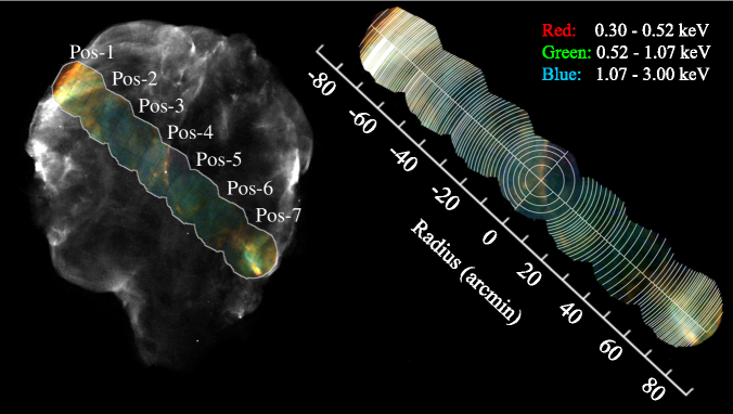
Figure 1: Left: Exposure-corrected ROSAT HRI image of the entire Cygnus Loop (black and white) overlaid with the XMM-Newton color images of the merged MOS1/2, PN data from all the XMM-Newton observations. Right: Spectral extraction regions overlaid on the XMM-Newton three-color image shown in left figure.

Figure 1 displays an exposure-corrected ROSAT HRI image of the entire Cygnus Loop (black and white) overlaid with the XMM-Newton color images of the merged MOS1/2, PN data from all the XMM-Newton observations. In this figure, we allocated color codes as red (0.3–0.52 keV), green (0.52–1.07 keV) and blue (1.07–3 keV). We see that the outer regions are reddish rather than bluish while the central region is in bluish.

The NE rim is the brightest in our field of view (FOV), showing a bright filament at $45^{\circ}$ to the radial direction corresponding to NGC6992. The SW rim is also bright in our FOV where there is a V-shape structure Aschenbach & Leahy (1999). In the center of the Loop, an X-ray bright filament runs through Pos-4 and Pos-5 forming a circular structure. In the ROSAT image, we can see it and find that it forms a large circle within the Cygnus Loop. In this way, there are many fine bright filaments in intensity. However, we find that there is a clear intensity variation along our scan path: dim in the center and bright in the rim.

Figure 2 shows spectra for seven pointings; each is the sum of the entire FOV. The NE rim (Pos-1) and the SW rim (Pos-7) show strong emission lines below 1 keV including O, Fe-L and Ne, while the center (Pos-4) shows strong emission lines from Si and S. We can see that the equivalent width of Si and S emission lines are bigger in the center and gradually decrease toward the rim. We show the comparison of spectra between Pos-1 and Pos-4 in figure 3. Prominent emission lines are O-He$\alpha$, O-Ly$\alpha$, Fe-L complex, Ne-He$\alpha$, Mg-He$\alpha$, Si-He$\alpha$, and S-He$\alpha$. We see that the emission line shapes for O are quite similar to each other while there is a big difference at higher energy band. Since the spectrum in the NE rim can be well represented by a single temperature plasma model Miyata et al. (1994), we need an extra component in the center.

3.2 Radial profile

Although there are many fine structures, no matter how finely we divide our FOV, each region would contain different plasma conditions due to the integration of the emission along the line of sight. Therefore, we concentrate on large scale structure along the scan path. First of all, we divided our FOV into two parts along the diameter: the north path and the south path. Then we divided them into many small annular sectors whose center is located at (20^h51^m34^s.7, 31^∘00^′00^′′), i.e., the center of the nominal position of Pos-4. There are 141 and 172 annular sectors for the north path and the south path, respectively. These small annular sectors, shown in figure 1, are divided such that each has at least 60,000 photons ($\sim$20,000 for MOS1/2 and $\sim$40,000 for PN) to equalize the statistics. We extracted the spectrum from each sector using the data set accumulated from blank sky observations as sky background. We have confirmed that the emission above 3 keV is statistically zero. In this way, we obtained 313 spectra. These sectors can be identified by the angular distance, “R”, from the center (east is negative and west is positive as shown in figure 1).

The width of the sector depends on R. The sector widths range from 3^′.8 to 0^′.2 in the north path and from 3^′.0 to 0^′.2 in the south path. The widest sectors are in Pos-4 due to its short exposure because of the background flare. The narrowest sectors are in the NE rim where the surface brightness is the highest.

3.3 Single temperature NEI model

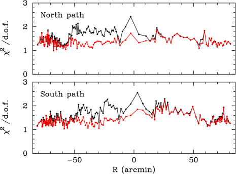
Figure 4: Distribution of the reduced-$\chi^{2}$  as a function of R along the north path (upper panel) and the south path (lower panel). The single-component model is shown in black and the two-component model is shown in red.

We fitted the spectrum for each sector with an absorbed non-equilibrium ionization (NEI) model with a single $kT_{\rm e}$, using the Wabs Morrison & McCammon (1983) and VNEI model (NEI version 2.0) Borkowski et al. (2001) in XSPEC v 12.3.1 Arnaud (1996)). We fixed the column density, $N_{\mathrm{H}}$ to be $4.0\times 10^{20}\mathrm{cm}^{-2}$ (e.g., Inoue et al. (1980), Kahn et al. (1980)). Free parameters were $kT_{\rm e}$; the ionization time scale, $\tau$ (a product of the electron density and the elapsed time after the shock heating); the emission measure (hereafter EM; EM = $\int n_{\rm e}n_{\rm H}d\ell$, where $n_{\rm H}$ and $n_{\rm e}$ are the number densities of hydrogens and electrons, $d\ell$ is the plasma depth); and abundances of C, N, O, Ne, Mg, Si, S, Fe, and Ni. We set abundances of C and N equal to that of O, that of Ni equal to Fe, and other elements fixed to the solar values Anders & Grevesse (1989). In the fitting process, we set 20 as the minimum counts in each spectral bin to perform the $\chi^{2}$ test. We determined the value of the minimum counts such that it did not affect the fitting results. Figure 4 shows the distribution of the reduced-$\chi^{2}$  in black as a function of R along both the north path and the south path. We found that values of reduced-$\chi^{2}$  for all the sectors are between 1.0 and 2.0. If we took into account a systematic error Nevalainen et al. (2003); Kirsch (2004) of 5 %, the reduced-$\chi^{2}$ was around 1.5 or less.

In general, values of the reduced-$\chi^{2}$  are a little higher in the central part of the Cygnus Loop. Miyata et al. (1994) observed the NE rim with ASCA and found that the spectra were well represented with a one-temperature VNEI model with a temperature gradient towards the inside. The Suzaku observation in the NE rim Miyata et al. (2007) reveals that the X-ray spectrum can be represented by a two-temperature model: one component is 0.2–0.35 keV and the other is 0.09–0.15 keV. In our fitting, the value of $kT_{\rm e}$ obtained is 0.2–0.25 keV. Therefore, we detected a hot component that Suzaku detected. There may be an additional component with low temperature that seems difficult to detect with XMM-Newton due to the relatively lower sensitivity below 0.5 keV compared to Suzaku.

The ASCA observation Miyata et al. (1994) also shows that the metal abundance in the NE rim is deficient. The authors concluded that the plasma in the NE-rim consists of the interstellar matter (ISM) rather than the ejecta. This is confirmed with the Suzaku observation Miyata et al. (2007) that indicates the abundances of C, N and O to be $\sim$0.1, 0.05 and 0.1 solar , respectively. We also obtained the metal deficiency in the NE rim data; the best-fit results are given in figure 5 (left) and in table LABEL:param1. Leahy (2004) measured the X-ray spectrum of the southwest region of the Cygnus Loop and reported that the oxygen abundance there is about 0.22 solar Leahy (2004). Therefore, the X-ray measurements of the Cygnus Loop show that the metal abundances are depleted.

Cartledge et al. (2004) measured the interstellar oxygen along 36 sight lines and confirmed the homogeneity of the O/H ratio within 800 pc of the Sun. We found that they measured it in the direction about $5^{\circ}$ away from the Cygnus Loop. The oxygen abundance they measured is about 0.4 times the solar value Anders & Grevesse (1989). Wilms et al. (2000) employed 0.6 of the total interstellar abundances for the gas-phase ISM oxygen abundance, and suggest that this depletion may be due to grains. Although the ISM near the Cygnus Loop may be depleted, the abundances are still much higher than what we obtained at the rim of the Cygnus Loop. It is difficult to explain such a low abundance of oxygen in material originating from the ISM. Therefore, the origin of the low metal abundance is open to the question. Since the Cygnus Loop is thought to have exploded in a pre-existing cavity, we can say that the cavity material shows low metal abundance. The abundance difference between our data and those from Suzaku may be due to the difference in the detection efficiency at low energy. Taking into account the projection effect, the plasma of the rim regions consists only of the cavity material while that of the inner regions consists both of the cavity material and of an extra component filling the interior of the Loop.

3.4 Two-temperature NEI model

To further constrain the plasma conditions, we applied a two-component NEI model with different temperatures. In this model, we added an extra component to the single temperature model. The extra component is also an absorbed VNEI model with $kT_{\rm e}$, $\tau$, and EM as free parameters. The metal abundances of the extra component are fixed to those determined at the NE rim so that the extra component represents the cavity material. Figure 4 shows reduced-$\chi^{2}$ values in red along the path. Applying the $F$-test with a significance level of 99% to determine whether or not an extra component is needed, we found that most of the spectra required a two-component model, particularly in the central part of the Loop. Sectors that do not require two-component model are mainly clustered in R$<$-65^′, +25${}^{\prime}<$R$<+40^{\prime}$, and +60${}^{\prime}<$R. Therefore, we considered that the outer sectors ($\mid$R$\mid>70^{\prime}$) can be safely represented by a one-component model while other sectors can be represented by a two-component model. In this way, we performed the analysis by applying a two-component VNEI model with different temperatures. We assumed that the low temperature component comes from the surrounding region of the Cygnus Loop and the high temperature component occupies the interior of the Loop.

We found that the values of reduced-$\chi^{2}$ are 1.0–1.8 even employing a two-component model. This is partly due to the systematic errors. Looking at the image in detail, there are fine structures within the sector. Furthermore, the spectrum from each sector is an integration along the line of sight. Since we only employ two VNEI plasma models, the values of reduced-$\chi^{2}$  are mainly due to the simplicity of the plasma model employed here. Therefore, we think that the plasma parameters obtained will represent typical values in each sector.

Figure 5 (right) and table LABEL:param2 shows an example result that comes from the sector at R=$+10^{\prime}$. Fixed parameters in the low $kT_{\rm e}$ component come from the fitting result at the NE rim obtained by Suzaku observations Uchida et al. (2006). Metal abundances for the high $kT_{\rm e}$ component show higher values by an order of magnitude than those of the low $kT_{\rm e}$ component, surely confirming that the high $kT_{\rm e}$ component is dominated by fossil ejecta.

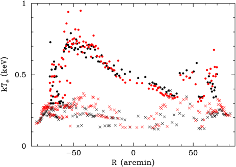
Figure 6: Temperature distributions of the two components as a function of position. Filled circles show the ejecta component, while crosses show the cavity component. Black show the north path and red shows the south path. Typical errors are $\pm$5% for both components.

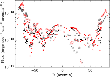
Figure 7: Flux distributions of the two components as a function of position. The marks in this figure are the same as those in figure 6.

Figure 6 shows temperatures as a function of position. The low $kT_{\rm e}$ component is in the temperature range of 0.12–0.34 keV while the high $kT_{\rm e}$ component is above 0.35 keV. There is a clear temperature difference where a two-component model is required rather than a single temperature model. The low $kT_{\rm e}$ component represents the cavity material surrounding the Cygnus Loop while the high $kT_{\rm e}$ component represents the fossil ejecta inside the Loop. Figure 7 shows the fluxes for the two components as a function of position. The low $kT_{\rm e}$ component shows clear rim brightening. The east part is stronger than the west part, showing asymmetry of the Loop. On the other hand, the high $kT_{\rm e}$ component has a relatively flat radial dependence. From the center to the SW, we see that the flux of the high $kT_{\rm e}$ component is stronger than that of the low $kT_{\rm e}$ component.

3.4.1 Distribution of the cavity material

As shown in figure 6, the low $kT_{\rm e}$ component shows relatively constant temperature with radius. The distribution of the flux shown in figure 7 shows peaks in the rim and relatively low values inside the Loop. There are some differences between the north path and the south path. The biggest one is a clear difference in peak position in the NE rim that is due to the bright filament at $45^{\circ}$ to the radial direction, as seen in figure 1. However, these two paths show a globally similar behavior in flux. Therefore, we can see that they are quite similar to each other from a large scale point of view.

We notice that there are many aspects showing asymmetry and non-uniformity. The NE half is stronger in intensity than the SW half. The flux in the inner part of the Loop shows relatively small values in the west half, particularly at +25${}^{\prime}<$R$<+40^{\prime}$. The NE half is brighter by a factor of 5–10 than the SW half. Furthermore, the SW half shows stronger intensity variation than the NE half. This suggests that the thickness of the cavity shell is far from uniform. The cavity shell in the SW half is much thinner than that in the NE half. Since we assumed the metal abundances of the low $kT_{\rm e}$ component equal to those of the NE rim, we can calculate the EM. Furthermore, we assumed the ambient density to be 0.7 cm^-3 based on the observation of the NE rim, and we estimate the mass of the low $kT_{\rm e}$ component to be 130 $\rm\,M_{\odot}$. However, we should note that there are is evidence that the SN explosion which produced the Cygnus Loop occurred within a preexisting cavity (e.g., Hester et al. 1994; Levenson et al. 1998; Levenson et al. 1999). The model predicts that the original cavity density, $n_{c}$, is related to the wall density $n_{s}$ by $n_{c}=5$. Assuming that $n_{0}$ equals the ambient density, $n_{s}$, we estimate $n_{c}$ to be 0.14 cm^-3. Then, we calculate the total mass in the preexisting cavity to be $\sim$25 M_⊙.

3.4.2 Ejecta distribution

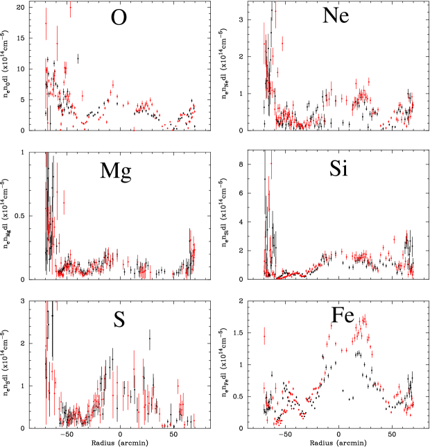
Figure 8: Distributions of EM for various metals (O(=C=N), Ne, Mg, Si, S, and Fe(=Ni)) in the ejecta. Black indicates the north path and red indicates the south path. Data points showing only upper limits are excluded in these figures.

The flux distribution from the ejecta along the path is shown with filled circles in figure 7. It has a relatively flat structure with two troughs around R=$-35^{\prime}$ and R=+50^′. Since we left the metal abundances as free parameters, we obtained distributions of EM of various metals (C=N=O, Fe=Ni, Ne, Mg, Si and S) in the ejecta. These are shown in figure 8, where black crosses trace the north path and red crosses trace along the south path. If we assume uniform plasma conditions along the line of sight, the EM represents the mass of the metal. Most elements show similar structure between the north path and the south path while there is a big discrepancy in Fe/Ni distribution at $-10^{\prime}<$ R $<+30^{\prime}$. In this region, the south path shows two times more abundant Fe/Ni than the north path. A similar discrepancy is seen in O ($-30^{\prime}<$ R $<-10^{\prime}$) and in Ne (at $-10^{\prime}<$ R $<+10^{\prime}$). Therefore, the distribution of metal abundance shows a north-south asymmetry along the path.

The distributions of O and Ne show a central bump and increase at the outer sectors. However, those of Mg, Si, S and Fe only show a central bump. The increase of O and Ne at the outer sectors indicates that the outer parts of the ejecta mainly consists of O and Ne and they may be well mixed. Similarly heavy elements, Mg, Si, S and Fe/Ni forming central bumps may show that they are well mixed. Therefore, a significant convection has occurred in the central bumps while an “onion-skin” structure remains in the outer sectors.

4 Discussion

The Cygnus Loop appears to be almost circular with a blowout in the south. The ROSAT image indicates no clear shell in this blowout region. Levenson et al. (1997) revealed that there is a thin shell left at the edge of the blowout region. Therefore, there is a small amount of cavity material in this region that surrounds the ejecta. This also indicates the non-uniformity of the cavity wall. If the cavity wall is thin, the ejecta can produce a blowout structure.

Looking at the component of the cavity material along our path shown in figure 7, the flux is very weak at +15${}^{\prime}<$R$<+40^{\prime}$. This indicates that the cavity wall is very thin in this region. When we calculate the flux ratio between the ejecta plasma and the cavity material, we find that the ratio becomes high (larger than 4) at +15${}^{\prime}<$R$<+35^{\prime}$ in the north path and +30${}^{\prime}<$R$<+35^{\prime}$ in the south path. Therefore, we guess that the thin shell region is larger in the north path than in the south path. This also shows the asymmetry between the north and the south as well as that between the east and the west. If the thin shell region corresponds to a blowout similar to that in the south blowout, this region must have a blowout structure along the line of sight either in the near side or far side or both. This structure roughly corresponds to Pos-5 and will extend further in the northwest direction. Looking at the ROSAT image in figure 1, we see a circular region with low intensity. It is centered at (20^h49^m11^s, 31^∘05^′20^′′) with a radius of 30^′. We guess that this circular region corresponds to a possible blowout in the direction of our line of sight. CCD observation just north of our path will answer this hypothesis.

We obtained EMs of O, Ne, Mg, Si, S, and Fe for the ejecta along the north path and the south path. Multiplying the EMs by the area of each sector, we obtained emission integral (hereafter EI, EI$=\int n_{\mathrm{e}}n_{\mathrm{H}}dV$, $dV$ is the X-ray-emitting volume) along the path. Since we only observed the limited area of the Cygnus Loop from the NE rim to the SW rim, we have to estimate the EIs for the entire remnant in order to obtain the relative abundances as well as the total mass of the ejecta. Therefore, we divide our observation region into four parts: left-north part, right-north part, left-south part, and right-south part. We assume that each part represents the average EIs of the corresponding quadrant of the Loop. In this way, we can calculate the total EIs for O, Ne, Mg, Si, S, and Fe that are described in table LABEL:emission_integral. The south quadrant, corresponding to the right-south path, contains the largest mass fraction of 31%, while the other quadrants contain 23% each. Then, we calculate the relative abundances of Ne, Mg, Si, S, and Fe to O in the entire ejecta. Since we cannot measure the abundance of light elements like He, it is quite difficult to estimate the absolute abundances. However, the relative abundance to O is robust.

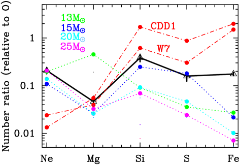
Figure 9: Number ratios of Ne, Mg, Si, S, and Fe relative to O of the high-$kT_{\rm e}$ component estimated for the entire Loop (black solid line). Dash-dotted red lines represent CDD1 and W7 model of Type-Ia Iwamoto et al. (1999). Dotted green, blue, light blue, and magenta lines represent core-collapse models whose progenitor masses are 13, 15, 20, and 25 $\rm\,M_{\odot}$, respectively Woosley & Weaver (1995).

Since the Cygnus Loop is believed to be a result from a core-collapse SN, we compared our data with core-collapse SN models. There are many theoretical results from various authors (e.g., Woosley & Weaver 1995; Thielemann et al. 1996; Rauscher et al. 2002; Tominaga et al. 2007). We also employed a SN Type Ia model Iwamoto et al. (1999) for comparison. We calculated the relative abundance for various elements to O and compared them with models. Figure 9 shows comparisons between the model calculations and our results where we picked up Woosley’s model with one solar abundance Anders & Grevesse (1989) for the core-collapse case Woosley & Weaver (1995). The Type Ia model yields more Si, S and Fe than our results, but less Ne. Models with massive stars produce better fits to our results than the Type Ia model. Among them, we found that the model with 15 $\rm\,M_{\odot}$ showed good fits to our results. They fit within a factor of two with an exception of Fe. We also noticed that the model with one solar abundance looked better fit than that with depleted abundance. Therefore, we can conclude that the Cygnus Loop originated from an approximately 15 $\rm\,M_{\odot}$ star with one solar abundance.

Assuming that the ejecta density is uniform along the line of sight, we estimate the total mass of the fossil ejecta to be 21 $\rm\,M_{\odot}$. In this calculation, we assumed that the electron density is equal to that of hydrogen and that the plasma filling factor is unity, although the fossil ejecta might be deficient in hydrogen. If it is the case, the total mass of the fossil ejecta reduces to $\sim$12, $\rm\,M_{\odot}$ whereas the relative abundances are not affected. The most suitable nucleosynthetic model predicts that the total mass ejected is about 6 $\rm\,M_{\odot}$ without H. Therefore, there might be a significant amount of contamination from the swept-up matter into the high-$kT_{\rm e}$ component, which we consider the ejecta. Otherwise, the assumption that the density of the ejecta is uniform might be incorrect since rim-brightening for the EMs of O, Ne, Mg, and Fe is clearly seen in Fig. 8. Non-uniformity reduces the filling factor and also the mass of the high-$kT_{\rm e}$ component.

There is observational evidence of the asymmetry of supernova explosions both for massive stars Leonard et al. (2006) and for Type Ia Motohara et al. (2006). We found that the ejecta plasma shows asymmetric structure between NE half and SW half. Ne and Fe are evenly divided while two thirds of O and Mg are in the NE half. On the contrary, two third of Si and S are in the SW half. We calculated the ejecta mass for each quadrant and found that the south quadrant contains the largest ejecta mass. Similar asymmetries are seen in other SNR, such as Puppis A, which shows asymmetric structure with O-rich, fast-moving knots (Winkler & Kirscher 1985; Winkler et al. 1988) . The central compact object in Puppis A is on the opposite side of the SNR from the O-rich, fast-moving knots Petre et al. (1996). If the asymmetry of the ejecta in the Cygnus Loop is similar to that of Puppis A, we may expect a compact object to be in the north direction.

5 Conclusion

We have observed the Cygnus Loop along the diameter from the NE rim to the SW rim employing XMM Newton. The FOV is divided into two paths: the north path and the south path. Then it is divided into many small annuli so that each annulus contains a similar number of photons to preserve statistics.

The spectra from the rim regions can be expressed by a one-$kT_{\rm e}$ component model while those in the inner region require a two-$kT_{\rm e}$ component model. The low $kT_{\rm e}$ plasma shows relatively low metal abundance and covers the entire FOV. It forms a shell that originates from the preexisting cavity. The high $kT_{\rm e}$ plasma shows high metal abundance and occupies a large part of the FOV. The origins of these two components are different: the high $kT_{\rm e}$ plasma with the high metal abundance must come from the ejecta while low $kT_{\rm e}$ plasma with low metal abundance must come from the cavity material. We find that the thickness of the shell is very thin in the south west part where, we guess, the ejecta plasma is blow out in the direction of our line of sight.

We estimate the mass of the metals. Based on the relative metal abundance, we find that the Cygnus Loop originated from a 15 $\rm\,M_{\odot}$ star. The distribution of the ejecta is asymmetric, suggesting an asymmetric explosion.

Table 1: Summary of the seven observations.

Obs. ID	Camera	Obs. Date	Coordinate (RA, DEC)	Effective Exposure
0082540101	MOS1	2002-11-25	20h55m23s.6, 31∘46′17′′.0	14.1 ksec
(Pos-1)	MOS2			14.1 ksec
	PN			5.6 ksec
0082540201	MOS1	2002-12-03	20h54m07s.4, 31∘30′51.4′′.0	14.4 ksec
(Pos-2)	MOS2			14.4 ksec
	PN			11.7 ksec
0082540301	MOS1	2002-12-05	20h52m51s.1, 31∘15′25′′.7	11.6 ksec
(Pos-3)	MOS2			11.6 ksec
	PN			9.1 ksec
0082540401	MOS1	2002-12-07	20h51m34s.7, 31∘00′00′′.0	4.9 ksec
(Pos-4)	MOS2			4.9 ksec
	PN			3.4 ksec
0082540501	MOS1	2002-12-09	20h50m18s.4, 30∘44′34′′.3	12.6 ksec
(Pos-5)	MOS2			12.6 ksec
	PN			10.0 ksec
0082540601	MOS1	2002-12-11	20h49m02s.0, 30∘28′16′′.1	11.5 ksec
(Pos-6)	MOS2			11.5 ksec
	PN			5.9 ksec
0082540701	MOS1	2002-12-13	20h47m45s.8, 30∘13′42′′.9	13.5 ksec
(Pos-7)	MOS2			13.5 ksec
	PN			7.5 ksec

Table 2: Spectral-fit parameters.

Parameter	region$-74.25$
$N_{\rm H}[10^{20}\,{\rm cm}^{-2}$]	4 (fixed)
$kT_{\rm e}$[keV]	0.23 $\pm$0.01
O(=C=N)	0.068 $\pm$0.002
Ne	0.17$\pm$0.01
Mg	0.14$\pm$0.03
Si	0.3$\pm$0.1
S	0.6$\pm$0.2
Fe(=Ni)	0.157$\pm$0.006
log$(\tau/\rm cm^{-3}\,sec)$	11.31 $\pm$0.02
EM1[$\times 10^{19}$ cm-5]	11.0${}^{+1.4}_{-0.5}$
$\chi^{2}$/d.o.f.	420/314
Note. Other elements are fixed to solar values.
The values of abundances are multiples of solar value.
The errors are in the range $\Delta\,\chi^{2}\,<\,2.7$ on one parameter.
1EM denotes emission measure, $\int n_{\mathrm{e}}n_{\mathrm{H}}d\ell$.

Table 3: Spectral-fit parameters.

Parameter	region$+10$
$N_{\rm H}[10^{20}\,{\rm cm}^{-2}$]	4 (fixed)
Low temperature component
$kT_{\rm e}$[keV]	0.20 $\pm$0.01
C	0.27 (fixed)
N	0.10 (fixed)
O	0.11 (fixed)
Ne	0.21 (fixed)
Mg	0.17 (fixed)
Si	0.34 (fixed)
S	0.17 (fixed)
Fe(=Ni)	0.20 (fixed)
log$(\tau/\rm cm^{-3}\,sec)$	$12<$
EM1[$\times 10^{18}$ cm-5]	1.34${}^{+0.03}_{--0.04}$
High temperature component
$kT_{\rm e}$[keV]	0.48 $\pm$0.01
O(=C=N)	$<$0.01
Ne	0.15 ${}^{+0.06}_{-0.07}$
Mg	0.21$\pm$0.08
Si	2.5$\pm$0.3
S	5$\pm$1
Fe(=Ni)	1.03$\pm$0.04
log$(\tau/\rm cm^{-3}\,sec)$	11.12$\pm$0.05
EM1[$\times 10^{19}$ cm-5]	0.094${}^{+0.005}_{-0.004}$
$\chi^{2}$/d.o.f.	531/377
Note. Other elements are fixed to solar values.
The values of abundances are multiples of solar value.
The errors are in the range $\Delta\,\chi^{2}\,<\,2.7$ on one parameter.
1EM denotes emission measure, $\int n_{\mathrm{e}}n_{\mathrm{H}}d\ell$.

Table 4: Calculated emission integral of the Cygnus Loop ejecta.

Element	1053 cm-3
O	7.4$\pm$0.5
Ne	1.5$\pm$0.2
Mg	0.34$\pm$0.1
Si	2.9$\pm$0.5
S	1.2$\pm$0.3
Fe	1.30$\pm$0.05

Figure 2: MOS1 spectra for the seven pointings; each is the sum of the entire FOV.

Figure 3: Comparison of spectra between Pos-1 (circles) and Pos-4 (triangles). They are equalized in intensity at O-He$\alpha$.

Figure 5: Left: An example spectrum that comes from the sector at R=$-74.25^{\prime}$. The best-fit curves are shown with solid lines and the lower panels show the residuals. Right: Same as left but for the sector at R=$+10^{\prime}$. Both the ejecta and cavity components are shown only for MOS1 spectrum as dashed lines.

References

- Anders & Grevesse (1989) Anders, E., & Grevesse, N. 1989, Geochim. Cosmochim. Acta, 53, 197
- Arnaud (1996) Arnaud, K. A. 1996, ASP Conf. Ser., 101, 17
- Aschenbach & Leahy (1999) Ashcehnbach, B. & Leahy, D. A. 1999, A&A, 341, 602
- Burrows & Hayes (1996) Burrows, Adam; Hayes, John, 1996, Physical Review Letters, 76, 352
- Blair et al. (2005) Blair, W. P., Sankrit, R., & Raymond, J. C., 2005, AJ, 129, 2268
- Borkowski et al. (2001) Borkowski, K. J., Lyerly, W. J., & Reynolds, S. P. 2001, ApJ, 548, 820
- Cartledge et al. (2004) Cartledge, S. I. B., Lauroesch, J. T., Meyer, D. M., & Sofia, U. J. 2004, ApJ, 613, 1037
- Dopita et al. (1977) Dopita, M. A., Mathewson, D. S., and Ford, V. L. 1977, ApJ, 214, 179
- Fujita et al. (2004) Fujita, Y., Sarazin, C. L., Reiprich, T. H., Andernach, H., Ehle, M., Murgia, M., Rudnich, L., & Slee, O. B. 2004, ApJ, 616, 157
- Ghavamian et al. (2001) Ghavamian, P., Raymond, John., Smith, R. C., & Hartigan, P. 2001, ApJ, 547, L995