Finite-size scaling of synchronized oscillation on complex networks

Abstract

The onset of synchronization in a system of random frequency oscillators coupled through a random network is investigated. Using a mean-field approximation, we characterize sample-to-sample fluctuations for networks of finite size, and derive the corresponding scaling properties in the critical region. For scale-free networks with the degree distribution $P(k)\sim k^{-\gamma}$ at large $k$, we found that the finite size exponent $\bar{\nu}$ takes on the value $5/2$ when $\gamma>5$, the same as in the globally coupled Kuramoto model. For highly heterogeneous networks ($3<\gamma<5$), $\bar{\nu}$ and the order parameter exponent $\beta$ depend on $\gamma$. The analytic expressions for these exponents obtained from the mean field theory are shown to be in excellent agreement with data from extensive numerical simulations.

I Introduction

The popularity of complex networks in the description of interactions among individuals in various biological and social contexts has inspired theoretical studies of ordering phenomena on networks in recent years ref:review_Dorogovtsev . The small-world properties of such networks, as emphasized first by Watts and Strogatz ref:WSnetworks , suggest that a simple mean-field (MF) description of the ordering transition is often appropriate ref:WSnetworks ; ref:review_Dorogovtsev . More complicated situations may arise as in, e.g., scale-free networks with a low degree exponent, where heterogeneity in the network topology smears out the transition significantly ref:hetero-DGM ; ref:FSS-HHP ; ref:Potts_Igloi ; ref:Ising_Leone ; ref:Percol_Havlin ; ref:DP_SFN . In general, randomness in network connections, which can be considered as a form of quenched disorder, can have a profound effect on the ordering process and the ensuing scaling behavior. This is a topic in the network research which has not been sufficiently explored so far.

Synchronization of coupled oscillators is a representative dynamical problem on complex networks ref:review_Dorogovtsev . By varying the coupling strength $J$ among the oscillators, various dynamical phenomena can be observed, ranging from independent oscillators at $J=0$ to fully synchronized state at $J>J_{f}$. The desynchronization threshold $J_{f}$ is an important property in many applications and its dependence on the network topology has been investigated in great detail ref:synch_networks . For coupled oscillators with a distribution of intrinsic frequencies ref:Winfree ; ref:Kuramoto ; ref:Pikovsky ; ref:Kiss , a finite fraction of the population can remain entrained in frequency even in the presence of a large number of run-away oscillators. The entrained cluster of oscillators disappears only at a (much) lower coupling strength $J_{c}$. Near the entrainment threshold $J_{c}$, strong fluctuations in various static and dynamic properties of the system are expected, as in usual critical phenomena.

The entrainment transition on scale-free networks with the degree distribution $P(k)\sim k^{-\gamma}$ has been treated analytically by several groups ref:SFN_mf ; ref:synch_SFN ; ref:MarylandGroup . It has been shown that, in the infinite size limit, the transition is expected at a finite coupling strength for $\gamma>3$, while the entrained cluster persists at any nonzero coupling strength for $\gamma\leq 3$. The critical exponent $\beta$ describing vanishing behavior of the order parameter on the supercritical side is shown to be equal to $1/2$ for $\gamma>5$ and $1/(\gamma-3)$ for $3<\gamma<5$ ref:synch_SFN .

For systems of finite size, the entrainment transition becomes blurred and rounded over a range of the coupling strength. In addition, randomness in the network topology, as well as the random choice of oscillator frequencies, introduces sample-to-sample variations in the entrainment threshold. A full description of the finite size effects, which requires a detailed characterization of dynamic fluctuations in specific samples, is currently not available ref:Strogatz ; ref:Acebron . Fortunately, in the case of the globally coupled Kuramoto model where the mean-field theory works well on the supercritical side, the sample-to-sample fluctuations of the order parameter can be characterized analytically ref:Hong_Entrainment . Comparison with numerical simulations indicates that temporal fluctuations of the order parameter only play a subdominant role in the broadening of the transition region due to finite size ref:Hong_Entrainment ; ref:HPT-BC . The success of this approach suggests a novel procedure to derive finite-size scaling (FSS) relations under a MF approximation.

In the present paper, we extend the above MF treatment to coupled random frequency oscillators on complex networks. Unlike the globally coupled case, the MF equations derived here are not expected to be exact due to the finite connectivity of individual vertices on the network. Nevertheless, as we show below, the FSS exponents obtained depend only on certain general properties of the network. We also present results from extensive simulations on uncorrelated scale-free networks. The numerically determined values of the exponents as a function of the degree exponent $\gamma$ of the network agree well with the analytic predictions. Our study indicates that the FSS at the entrainment transition on uncorrelated scale-free networks is also governed by fluctuations in the distribution of intrinsic oscillator frequencies, with temporal order parameter fluctuations playing a less dominant role.

The paper is organized as follows. In Sec. II we introduce the dynamic model and derive the mean-field equations. Section III contains a treatment of the mean-field equations in the neighborhood of the entrainment transition. A finite-size scaling form for the order parameter is obtained. Results from numerical simulations of the model are presented in Sec. IV and compared with the analytic predictions. Section V contains a brief summary of our results.

II The Model and Mean-field Equations

II.1 The model

An undirected network of $N$ vertices is defined by the adjacency matrix $\{a_{ij}\}$, where $a_{ij}=1$ if two vertices $i$ and $j$ are connected and 0 otherwise. The degree of a vertex $i$ is the number of vertices connected to $i$, denoted by $k_{i}=\sum_{j}a_{ij}$. To each vertex $i$ we associate an oscillator whose dynamics is described by the equation of motion for the phase $\phi_{i}$,

$$\dot{\phi}_{i}=\omega_{i}-J\sum_{j=1}^{N}a_{ij}\sin(\phi_{i}-\phi_{j}),$$ (1)

where $\omega_{i}$ is the intrinsic frequency of the oscillator. The second term on the right-hand side of Eq. (1) denotes coupling to neighboring oscillators on the network with a positive strength ($J>0$).

In this paper, the oscillator frequencies $\omega_{i}$ in a given sample are drawn independently from a distribution $g(\omega)$ which is assumed to be a smooth function and symmetric about its maximum at $\omega=0$. In addition, we shall limit ourselves to random networks with no degree-degree correlation among neighboring vertices. An algorithm that generates such a network with no self linking nor multiple links between vertices is discussed in Ref. ref:Catanzaro . The numerical results presented in Sec. IV are for scale-free networks generated using the static model of Ref. ref:SNUstatic_SFN .

II.2 The mean-field approximation

At sufficiently strong coupling, the system described by Eq. (1) exhibits a synchronization phenomenon where a finite fraction of oscillators in the system become entrained in frequency. Transition to the random state at a critical coupling strength $J_{c}$ has been considered at the mean-field level by several authors ref:SFN_mf ; ref:synch_SFN ; ref:MarylandGroup . To understand the general idea behind such an approach, let us first introduce a set of instantaneous local fields defined by

$$H_{i}e^{i\theta_{i}}\equiv\sum_{j}a_{ij}e^{i\phi_{j}},$$ (2)

where $H_{i}\geq 0$ denotes the amplitude and $\theta_{i}$ the phase, respectively. Eq. (1) can now be written in a more suggestive form,

$$\dot{\phi}_{i}=\omega_{i}-H_{i}J\sin(\phi_{i}-\theta_{i}).$$ (3)

As usual, the mean-field approximation decouples the set of $N$ dynamical equations by replacing $H_{i}$ and $\theta_{i}$ with suitable time-averaged quantities which are then determined in a self-consistent manner. Unlike the globally coupled Kuramoto model, such a mean-field treatment is not exact due to the finite connectivity of individual oscillators on the network, so dynamic fluctuations are not averaged out even for an infinite system. However, provided the network is sufficiently well connected (as compared to fragmentation into local “communities”), and because of its small-world properties, once a cluster of entrained oscillators is formed, it will affect the dynamics of all oscillators in the system through a global “ordering field” $H\exp(i\theta)$. The precise effect of the global field on individual oscillators is subject to renormalization by the local community of a given oscillator. For a well-connected network, it is reasonable to expect that renormalization of oscillator’s response function does not change qualitatively results of the mean-field theory where such effects are ignored. This is to be confirmed by numerical investigations.

With the above caveat, let us proceed to the derivation of the mean-field equations, with particular emphasis on the finite size effect. The key approximation we introduce is to replace each phase factor $e^{i\phi_{j}}$ in the sum of Eq. (2) by the global ordering field $H\exp(i\theta)$ acting through the edge connecting vertices $i$ and $j$. Equation (3) now becomes

$$\dot{\phi}_{i}=\omega_{i}-k_{i}HJ\sin(\phi_{i}-\theta).$$ (4)

Consider a steady-state situation with a constant $H$ and a linearly advancing $\theta=\Omega t$, where $\Omega$ is the phase velocity of the entrained cluster. From Eq. (4), the oscillator at vertex $i$ is entrained with

$$\phi_{i}=\theta+\sin^{-1}[(\omega_{i}-\Omega)/(k_{i}HJ)]$$ (5)

if $|\omega_{i}-\Omega|\leq k_{i}HJ$, and detrained otherwise. In the latter case, the time averaged value of $e^{i(\phi_{i}-\theta)}$ is given by

$$\overline{e^{i(\phi_{i}-\theta)}}=i\Bigl{(}\frac{\omega_{i}-\Omega}{k_{i}HJ}\Bigr{)}\Bigl{[}1-\sqrt{1-\Bigl{(}\frac{k_{i}HJ}{\omega_{i}-\Omega}\Bigr{)}^{2}}\Bigr{]}.$$ (6)

Here and elsewhere the overline bar denotes time average.

The self-consistent equations for $H$ and $\Omega$ are obtained by setting $H$ equal to the average of $\overline{e^{i(\phi_{i}-\theta)}}$ over all edges of the network. Since each vertex $i$ contributes $k_{i}$ times to the average, we may write

$$H=\frac{\sum_{i}k_{i}\overline{e^{i(\phi_{i}-\theta)}}}{\sum_{i}k_{i}}=\frac{1}{N}\sum_{i=1}^{N}\frac{k_{i}}{\langle k\rangle}\overline{e^{i(\phi_{i}-\theta)}}.$$ (7)

Here $\langle k\rangle$ is the average degree of a vertex in the network. Substituting Eqs. (5) and (6) into Eq. (7), and separating out real and imaginary parts, we obtain

$$H = \frac{1}{N}\sum_{i=1}^{N}\frac{k_{i}}{\langle k\rangle}\sqrt{1-f_{i}^{2}}\Theta(1-|f_{i}|),$$ (8)

$$0 = \sum_{i=1}^{N}(\omega_{i}-\Omega)\Bigl{[}1-\sqrt{1-f_{i}^{-2}}\Theta(|f_{i}|-1)\Bigr{]},$$ (9)

where $f_{i}=(\omega_{i}-\Omega)/(k_{i}HJ)$, and $\Theta(x)$ is the Heaviside step function which takes the value 1 for $x\geq 0$ and $0$ otherwise.

Equations (8) and (9) are our mean-field equations for a given network of $N$ oscillators with a particular set of intrinsic frequencies $\{\omega_{i}\}$. They are invariant under a uniform shift of all oscillator frequencies (with a corresponding change in $\Omega$).

At any value of $J$, Eqs. (8) and (9) admit a trivial solution $H=0$ (with arbitrary $\Omega$). In the next section, we shall analyze nontrivial solutions that appear above the entrainment threshold $J_{c}$, with particular attention on sample-to-sample variations when $N$ is finite.

III Solution of the mean-field equations

From Eqs. (8) and (9) it is obvious that the solution for $H$ depends not only on the coupling strength $J$ but also on the particular choice of the intrinsic frequencies $\{\omega_{i}\}$ as well as the particular network topology in a given sample. For sufficiently large $N$, it is possible to give a statistical description of the sample-to-sample fluctuations. As we show below, the analysis also yields the finite-size scaling of the critical properties in the neighborhood of the entrainment transition. By symmetry we shall seek a solution at $\Omega=0$ and ignore weak finite-size corrections which do not alter our main conclusions.

III.1 Self-averaging in the infinite size limit

To proceed, let us write Eq. (8) in a symbolic form,

$$H=\tilde{\Psi}(H),$$ (10)

where

$$\tilde{\Psi}(H)\equiv\frac{1}{N}\sum_{i=1}^{N}\frac{k_{i}}{\langle k\rangle}\sqrt{1-\Bigl{(}\frac{\omega_{i}}{k_{i}HJ}\Bigr{)}^{2}}\Theta\Bigl{(}1-\frac{|\omega_{i}|}{k_{i}HJ}\Bigr{)}.$$ (11)

Terms in the sum can be grouped according to their degree $k_{i}$. When the network size $N\rightarrow\infty$, the number of terms in each group at a given $k$ grows linearly with $N$, and hence the self-averaging over the distribution $g(\omega)$ is expected. This consideration leads to the result,

$$\Psi(H)\equiv\lim_{N\rightarrow\infty}\tilde{\Psi}(H)=\langle\tilde{\Psi}(H)\rangle=\frac{1}{\langle k\rangle}\sum_{k}P(k)ku(kHJ).$$ (12)

Here $P(k)$ is the degree distribution of vertices on the network, and

$$u(x)=\int_{-x}^{x}d\omega g(\omega)\sqrt{1-\omega^{2}/x^{2}}$$ (13)

is a monotonically increasing function of $x$ which approaches 1 as $x\rightarrow\infty$. For small $x$, $u(x)\simeq\frac{\pi}{2}g(0)x+\frac{\pi}{16}g^{\prime\prime}(0)x^{3}$.

We now consider the behavior of $\Psi(H)$ at small $H$, assuming $\langle k^{2}\rangle=\sum_{k}k^{2}P(k)$ to be finite (i.e., $P(k)$ falls off faster than $k^{-3}$ at large $k$). To facilitate the analysis, we write

$$u(x)=ax-\hat{u}(x),$$ (14)

where $a=\frac{\pi}{2}g(0)$ and $\hat{u}(x)\simeq-{\pi\over 16}g^{\prime\prime}(0)x^{3}$ for small $x$. Substituting Eq. (14) into Eq. (12), we obtain

$$\Psi(H)=a\frac{\langle k^{2}\rangle}{\langle k\rangle}JH-\hat{\Psi}(H),$$ (15)

where

$$\hat{\Psi}(H)=\frac{1}{\langle k\rangle}\sum_{k}P(k)k\hat{u}(kHJ).$$ (16)

The functional form of $\hat{\Psi}(H)$ at small $H$ depends on the tail of the degree distribution $P(k)$. If $P(k)$ falls faster than $k^{-5}$ at large $k$, we may use the small $x$ expansion of $\hat{u}(x)$ to obtain

$$\hat{\Psi}(H)\simeq c_{0}\frac{\langle k^{4}\rangle}{\langle k\rangle}(JH)^{3},$$ (17)

where $c_{0}=-({\pi/16})g^{\prime\prime}(0)$ is a positive constant. On the other hand, if $P(k)\simeq Ak^{-\gamma}$ at large $k$ with $3<\gamma<5$, $\langle k^{4}\rangle$ diverges and the above expansion becomes invalid. Instead, contributions to the sum in Eq. (16) come mainly from vertices with $k\sim(JH)^{-1}$. Since the fraction of vertices in this degree range is proportional to $k^{-\gamma+1}$, and each contributing an amount $k$ to the sum, we estimate $\hat{\Psi}(H)\sim(JH)^{\gamma-2}$ in this case. More precisely, replacing the sum over $k$ by an integral, we obtain

$$\hat{\Psi}(H) \simeq \frac{1}{\langle k\rangle}\int_{0}^{\infty}dkP(k)k\hat{u}(kHJ)$$ (18)

$$\simeq \frac{1}{\langle k\rangle}\int_{0}^{\infty}dkAk^{-\gamma+1}\hat{u}(kHJ)$$

$$= c_{1}(JH)^{\gamma-2}.$$

Here $c_{1}=A{\langle k\rangle}^{-1}\int_{0}^{\infty}dxx^{-\gamma+1}\hat{u}(x)$ is another positive constant.

III.2 Sample-to-sample variations in a finite network

To work out the statistics of the sample-to-sample fluctuation $\delta\tilde{\Psi}(H)\equiv\tilde{\Psi}(H)-\Psi(H)$, we note that $\tilde{\Psi}(H)$ can be viewed as the mean value of the random variable,

$$\eta(\omega,k)=\frac{k}{\langle k\rangle}\sqrt{1-\Bigl{(}\frac{\omega}{kHJ}\Bigr{)}^{2}}\Theta\Bigl{(}1-\frac{|\omega|}{kHJ}\Bigr{)}$$ (19)

over $N$ realizations. From the central limit theorem, we expect $\delta\tilde{\Psi}(H)$ to satisfy the Gaussian distribution with zero mean and a variance given by

$$\langle(\delta\tilde{\Psi})^{2}\rangle=\frac{1}{N}\bigl{(}\langle\eta^{2}\rangle-\langle\eta\rangle^{2}\bigr{)}\equiv\frac{D(H)}{N}.$$ (20)

As $\langle\eta\rangle=\Psi(H)\sim H$ at small $H$, we only need to focus on

$$\langle\eta^{2}\rangle=\sum_{k}P(k)\frac{k^{2}}{\langle k\rangle^{2}}\int_{-kHJ}^{kHJ}d\omega g(\omega)\Bigl{[}1-\Bigl{(}\frac{\omega}{kHJ}\Bigr{)}^{2}\Bigr{]}$$ (21)

close to the transition. If $P(k)$ falls faster than $k^{-4}$ at large $k$, the above expression can be easily evaluated at small $H$ to give

$$D(H)\simeq\langle\eta^{2}\rangle\simeq\frac{4\langle k^{3}\rangle}{3\langle k\rangle^{2}}g(0)JH.$$ (22)

On the other hand, if $P(k)\simeq Ak^{-\gamma}$ with $3<\gamma<4$, we may replace the sum over $k$ by an integral which yields

$$D(H)\simeq d_{1}(JH)^{\gamma-3},$$ (23)

where $d_{1}=A\langle k\rangle^{-2}\int_{0}^{\infty}duu^{2-\gamma}\int_{-u}^{u}d\omega g(\omega)(1-\omega^{2}/u^{2})$ is another positive constant.

Summarizing the above results, in the neighborhood of the entrainment transition, we may write the self-consistent equation (10) for $H$ in the form,

$$H=(J/J_{c})H-c(JH)^{p}+d(JH)^{q/2}N^{-1/2}\xi,$$ (24)

where $c$ and $d$ are positive constants, and $J_{c}=2\langle k\rangle/(\pi g(0)\langle k^{2}\rangle)$ (mean-field value) is the critical coupling strength at the transition. The term $\xi$ is a Gaussian random variable with zero mean and unit variance that represents the combined effect of random frequency and network realizations in a given sample. The exponents $p=3$ and $q=1$ when the degree distribution $P(k)$ decays sufficiently fast at large $k$. For power-law distributions $P(k)\sim k^{-\gamma}$, $p$ switches to the value $\gamma-2$ for $\gamma<5$. Similarly, $q$ switches to the value $\gamma-3$ for $\gamma<4$.

III.3 Finite-size scaling

The network size $N$ enters Eq. (24) through the last , where $\xi$ varies from sample to sample. At $J=J_{c}$, a positive $\xi$ (50% of the samples) yields a solution $H\sim N^{-1/(2p-q)}$, quite a bit larger than the value $N^{-1/2}$ due to dynamic fluctuations on the detrained side ref:Daido . In addition, one can easily verify that the term $\xi$ affects the solution significantly when $J$ is within a distance of order $N^{-(p-1)/(2p-q)}$ from $J_{c}$. These properties are summarized in the scaling solution to Eq. (24),

$$H=N^{-\beta/\bar{\nu}}f\bigl{(}(J-J_{c})N^{1/\bar{\nu}}\bigr{)},$$ (25)

where the exponents $\beta=1/(p-1)$ and $\bar{\nu}=(2p-q)/(p-1)$. Unlike the usual FSS expression for pure systems, the scaling function $f(x)$ varies from sample to sample.

Using the above values for $p$ and $q$, we obtain the following results for the critical exponents in case of uncorrelated scale-free networks,

$$(\beta,~{}\bar{\nu})=\left\{\begin{array}[]{cccl}\frac{1}{2},&\frac{5}{2},&\qquad\mbox{$\gamma>5$;}\\ \frac{1}{\gamma-3},&\frac{2\gamma-5}{\gamma-3},&\qquad\mbox{$4<\gamma<5$;}\\ \frac{1}{\gamma-3},&\frac{\gamma-1}{\gamma-3},&\qquad\mbox{$3<\gamma<4$.}\end{array}\right.$$ (26)

In simulation studies, the order parameter

$$\Delta=\frac{1}{N}\sum_{i=1}^{N}\overline{e^{i(\phi_{i}-\theta)}}$$ (27)

is usually measured. From the solution to the mean-field equation (4), we obtain

$$\Delta=\frac{1}{N}\sum_{i=1}^{N}\sqrt{1-\Bigl{(}\frac{\omega_{i}}{k_{i}HJ}\Bigr{)}^{2}}\Theta\Bigl{(}1-\frac{|\omega_{i}|}{k_{i}HJ}\Bigr{)}.$$ (28)

Following the same procedure as above in the calculation of $\Psi(H)$, we obtain at small $H$,

$$\Delta\simeq a\langle k\rangle JH+d_{2}(JH)^{1/2}N^{-1/2}\tilde{\xi},$$ (29)

where $d_{2}=[(4/3)g(0)\langle k\rangle]^{1/2}$ and $\tilde{\xi}$ is another Gaussian random variable. The finite-size term here is negligible even at the transition. Hence the scaling behavior of $\Delta$ is the same as that of $H$.

We note that the expressions for the FSS exponent $\bar{\nu}$ in Eq. (26) differ from those obtained by Lee ref:synch_SFN based on a cluster analysis but without considering sample-to-sample fluctuations. In fact, $\bar{\nu}$ obtained here is always larger than that in ref:synch_SFN for any $\gamma$. This observation suggests that the broadening of the transition region by the random nature of oscillator frequencies and network connectivity is more significant than other effects such as those considered in Ref. ref:synch_SFN .

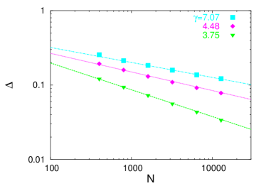
Figure 1: (Color online) Critical decay of $\Delta$ at the critical point $J_{c}$ as a function of $N$ for $\gamma=7.07,4.48,3.75$, where $J_{c}=1.86(2),1.57(4),1.17(3)$, respectively. Lines are drawn with slopes of $-\beta/\bar{\nu}$ given by the theoretical prediction, Eq. (26).

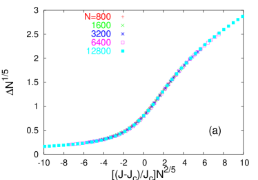
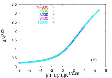
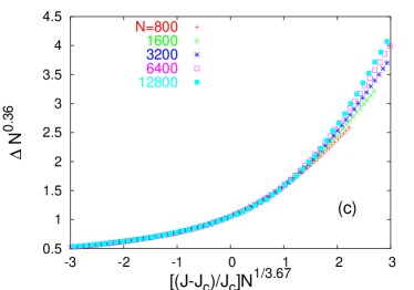
Figure 2: (Color online) Scaling plot of $\Delta$ for $N=800,1600,\cdots,12800$ with (a) $\gamma=7.07$, using $\beta/\bar{\nu}=1/5$ and $\bar{\nu}=5/2$, (b) $\gamma=4.48$, using $\beta/\bar{\nu}=0.25$ and $\bar{\nu}=2.68$, and (c) $\gamma=3.75$, using $\beta/\bar{\nu}=0.36$ and $\bar{\nu}=3.67$.

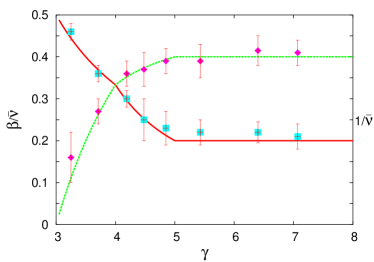
Figure 3: (Color online) $\beta/\bar{\nu}$ (box) and $1/\bar{\nu}$ (triangle) are plotted as a function of the degree exponent $\gamma$, showing a good consistency with the theoretical prediction represented by the full line ($\beta/\bar{\nu}$) and the dotted one ($1/\bar{\nu}$), respectively.

IV Numerical results

To test the validity of our MF analysis, we have performed extensive numerical simulations on the system governed by Eq. (1). Scale-free networks used in the simulation are generated following Ref. ref:SNUstatic_SFN , up to a system size $N=12800$. The intrinsic frequencies of oscillators are drawn independently from the Gaussian distribution $g(\omega)=(2\pi\sigma)^{-1/2}\exp(-\omega^{2}/2\sigma^{2})$ with unit variance ($\sigma^{2}=1$). The Heun’s method ref:Heun , with a discrete time step $\delta t=0.01$, is used to integrate numerically Eq. (1). Typically, the motion is followed for $N_{t}=4\times 10^{4}$ time steps, with the initial condition $\phi_{i}=0$ for all $i$. Data from the first $N_{t}/2$ steps are discarded in measuring the time average of various quantities of interest. For each network size, approximately $10^{4}$ independent runs are performed, with different realizations of the intrinsic frequencies as well as network connectivity to obtain sample averages.

To characterize the entrainment transition numerically, we have focused on the order parameter defined by Eq. (27), or more precisely, $\Delta=\langle\overline{\Delta_{t}}\rangle$, where $\Delta_{t}=|\frac{1}{N}\sum_{j=1}^{N}\exp(i\phi_{j})|$ at time $t$ and $\langle\cdots\rangle$ denotes the sample average for a given size. The critical coupling strength $J_{c}$ is estimated from the crossing point in the plot $\Delta N^{\epsilon}$ versus $J$, varying the exponent $\epsilon$. This value for $J_{c}$ is checked against crossing of the Binder cumulants at different size defined by $B_{\Delta}=1-\frac{1}{3}\langle\overline{\Delta_{t}^{4}}/\overline{\Delta_{t}^{2}}^{2}\rangle$ ref:HPT-BC , and compared with the behavior of the dynamic susceptibility $\chi=N\langle\overline{\Delta_{t}^{2}}-\overline{\Delta_{t}}^{2}\rangle$. At the critical point $J=J_{c}$, the order parameter $\Delta$ exhibits a power law: $\Delta\sim N^{-\beta/\bar{\nu}}$, which provides an alternative way for checking the critical value as well as determining the exponent ratio $\beta/\bar{\nu}$. With the values of $\beta/\bar{\nu}$ so obtained, we estimate the value of the FSS exponent $\bar{\nu}$ from the scaling plots of $\Delta N^{\beta/\bar{\nu}}$ against $(J-J_{c})N^{1/\bar{\nu}}$ for a broad range of systems sizes $N$, adjusting $\bar{\nu}$ to achieve the best data collapse in the critical region.

Figure 1 shows the critical decay of the order parameter $\Delta$ at $J_{c}$ as a function of $N$ on log-log scale. The critical values of $J$ are given by $J_{c}=1.86(2),1.57(4)$, and $1.17(3)$ for $\gamma=7.07,4.48$, and $3.75$, respectively. Each set of data points at a given $\gamma$ fall nicely on a straight line corresponding to the anticipated power law behavior $\Delta(J_{c})\sim N^{-\beta/\bar{\nu}}$, and the slope shows very good agreement with the predicted value for $\beta/\bar{\nu}$ according to Eq. (26).

Figure 2 shows the scaling plots of the order parameter $\Delta$ for various system sizes at three different values of $\gamma$. In each case, the theoretically predicted values given by Eq. (26) are used to scale the horizontal and vertical axes. The data collapse is nearly perfect for $\gamma=7.07$ and $4.48$, and satisfactory for $\gamma=3.75$.

Finally, we present in Fig. 3 results for $\beta/\bar{\nu}$ and $\bar{\nu}$ determined following the procedure described above at various values of $\gamma$. Error bars are obtained from uncertainties in the procedure. The two lines correspond to our MF predictions. The agreement is generally good.

V Conclusions and discussion

In this paper, we investigated the effect of fluctuations in the frequency distribution on the entrainment transition of a system of coupled random frequency oscillators. Self-consistent equations for the global ordering field are derived for any given oscillator population on a complex network. Statistical properties of the solution to these equations in an ensemble of such networks of oscillators are determined. The analysis enables us to derive a finite-size scaling expression for the entrainment order parameter. Comparison with numerical integration of dynamical equations on scale-free networks shows that the mean-field description correctly captures the finite-size scaling behavior exhibited by the sample-averaged order parameter $\Delta$. The values of exponents $\beta$ and $\bar{\nu}$ which best describe the numerical data show excellent agreement with the predicted ones from the mean-field theory.

For scale-free networks with a degree exponent $\gamma>5$, our result for the exponents $\beta=1/2$ and $\bar{\nu}=5/2$ is the same as the globally coupled Kuramoto model. Randomness in the network connection does not appear to affect these values. On this ground we expect the result to apply to randomly connected networks with a bounded degree, to the Erdös and Rényi network ref:Erdos , as well as to the small-world networks of Watts and Strogatz ref:WSnetworks . However, the finite connectivity of oscillators on the network implies that the dynamic fluctuations are not averaged out and can at least renormalize the entrainment threshold $J_{c}$ given by the mean-field theory. In this regard, analytic derivation of the sample-dependent, self-consistent equation (24) beyond the mean-field approximation would be desirable.

This work was supported by Korea Research Foundation Grant funded by the Korean Government (MOEHRD) (KRF-2006-331-C00123) and by the Research Grants Council of the HKSAR through grant 202107.

References

- (1) For a recent review, see S. N. Dorogovtsev and A. V. Goltsev, cond-mat/0705.0010 (2007) and references therein.
- (2) D. J. Watts and S. H. Strogatz, Nature (London) 393, 440 (1998); D. J. Watts, Small Worlds (Princeton University Press, Princeton, New Jersey, 1999).
- (3) S.N. Dorogovtsev, A.V. Goltsev, and J.F.F. Mendes, Phys. Rev. E 66, 016104 (2002); Eur. Phys. J. B 38, 177 (2004); A.V. Goltsev, S.N. Dorogovtsev, and J.F.F. Mendes, Phys Rev. E 67, 026123 (2003).
- (4) H. Hong, M. Ha, and H. Park, Phys. Rev. Lett. 98, 258701 (2007).
- (5) F. Iglói and L. Turban, Phys. Rev. E 66, 036140 (2002).
- (6) M. Leone, A. Vázquez, A. Vespignani, and R. Zecchina, Eur. Phys. J. B 28, 191 (2002).
- (7) R. Cohen, K. Erez, D. ben-Avraham, and S. Havlin, Phys. Rev. Lett. 85, 4626 (2000).
- (8) R. Pastor-Satorras and A. Vespignani, Phys. Rev. Lett. 86, 3200 (2001); Phys. Rev. E 63, 066117 (2001); M. Karsai, R. Juhasz, and F. Iglói, ibid. 73, 036116 (2006).
- (9) M. Barahona and L. M. Pecora, Phys. Rev. Lett. 89, 054101 (2002); M. Timme, F. Wolf, and T. Geisel, ibid. 89, 258701 (2002); T. Nishikawa, A.E. Motter, Y.-C. Lai, and F.C. Hoppensteadt, ibid. 91, 014101 (2003); H. Hong, B. J. Kim, M. Y. Choi, and H. Park, Phys. Rev. E 69, 067105 (2004).
- (10) A. T. Winfree, The Geometry of Biological Time (Springer-Verlag, New York, 1980); J. Theor. Biol. 16, 15 (1967).
- (11) Y. Kuramoto, in Proceedings of the International Symposium on Mathematical Problems in Theoretical Physics, edited by H. Araki (Springer-Verlag, New York, 1975); Chemical Oscillations, Waves, and Turbulence (Springer-Verlag, Berlin, 1984); Y. Kuramoto and I. Nishikawa, J. Stat. Phys. 49, 569 (1987).
- (12) A. S. Pikovsky, M. Rosenblum, and J. Kurths, Synchronization: A Universal Concept in Nonlinear Science (Cambridge University Press, Cambridge, 2001).
- (13) I. Z. Kiss, Y. M. Zhai, and J. L. Hudson, Science 296, 1676 (2002); Phys. Rev. Lett. 94, 248301 (2005).
- (14) T. Ichinomiya, Phys. Rev. E 70, 026116 (2004).
- (15) D.-S. Lee, Phys. Rev. E 72, 026208 (2005); E. Oh, D.-S. Lee, B. Kahng, and D. Kim, Phys. Rev. E 75, 011104 (2007).
- (16) J. G. Restrepo, E. Ott, and B. R. Hunt, Phys. Rev. E 71, 036151 (2005).
- (17) S. H. Strogatz, Physica D 143, 1 (2000).
- (18) For a recent review, see J. A. Acebrón, L. L. Bonilla, C. J. P. Vicente, and F. Ritort, Rev. Mod. Phys. 77, 137 (2005); and references therein.
- (19) H. Hong, H. Chaté, H. Park, and L.-H. Tang, Phys. Rev. Lett. (to appear); cond-mat/0701646.
- (20) H. Hong, H. Park, and L.-H. Tang, J. Korean Phys. Soc. 49 L1885 (2006).
- (21) M. Catanzaro, M. Boguñá, and R. Pastor-Satorras, Phys. Rev. E 71, 027103 (2005).
- (22) K.-I. Goh, B. Kahng, and D. Kim, Phys. Rev. Lett. 87, 278701 (2001).
- (23) H. Daido, Prog. Theor. Phys. 75, 1460 (1986); ibid. 77, 622 (1987).
- (24) See. e.g., R. L. Burden and J. D. Faires, Numerical Analysis (Brooks-Cole, Pacific Grove, 1997), p.280.
- (25) P. Erdös and A. Rényi, Publicationes Mathematicae Debrencen 6, 290 (1959).