Star Formation Density and H$\alpha$ Luminosity Function of an Emission Line Selected Galaxy Sample at $z\sim 0.24$

Abstract

We use narrowband imaging (FWHM $=70$ Å) to select a sample of emission line galaxies between $0.20\lesssim z\lesssim 1.22$ in two fields covering 0.5 sq. deg. We use spectroscopic follow-up to select a sub-sample of H$\alpha$ emitting galaxies at $z\sim 0.24$ and determine the H$\alpha$ luminosity function and star formation density at $z\sim 0.24$ for both of our fields. Corrections are made for imaging and spectroscopic incompleteness, extinction and interloper contamination on the basis of the spectroscopic data. When compared to each other, we find the field samples differ by $\Delta\alpha=0.2$ in faint end slope and $\Delta\log[L^{*}(\mathrm{{\mathrm{erg\,s^{-1}}}})]=0.2$ in luminosity. In the context of other recent surveys, our sample has comparable faint end slope, but a fainter $L^{*}$ turn-over. We conclude that systematic uncertainties and differences in selection criteria remain the dominant sources of uncertainty between H$\alpha$ luminosity functions at this redshift.

We also investigate average star formation rates as a function of local environment and find typical values consistent with the field densities that we probe, in agreement with previous results. However, we find tentative evidence for an increase in star formation rate with respect to the local density of star forming galaxies, consistent with the scenario that galaxy-galaxy interactions are triggers for bursts of star formation.

1 Introduction

It is now widely accepted that the amount of star formation in Universe as a whole has increased since the formation of the first galaxies, peaking around redshifts $z\sim 2-3$ and subsequently declining by a factor of ten (e.g. Hopkins, 2004, and references therein). Cosmic star formation history provides strong constraints on models of galaxy formation and evolution (Pei et al., 1999; Somerville et al., 2001), because it directly traces the accumulation of stellar mass and metal fraction (Pei & Fall, 1995; Madau et al., 1996) to their present-day values (Cole et al., 2001; Panter et al., 2003). Its rapid decline over the past 8 Gyr is consistent with “downsizing” scenarios (Cowie et al., 1996) in which the more massive galaxies have produced their stellar mass at earlier times than the less massive galaxies (Heavens et al., 2004; Juneau et al., 2005; Thomas et al., 2005; Fardal et al., 2006). The star formation history of the universe has also been used to constrain allowable stellar initial mass functions (Baldry & Glazebrook, 2003; Hopkins & Beacom, 2006) and cosmic supernova rates (Gal-Yam & Maoz, 2004; Daigne et al., 2006).

Star forming galaxies exhibit a strong UV continuum courtesy of newly formed OB stars in sites of star formation. This newborn population can be inferred from the UV directly (e.g. Treyer et al., 1998; Lilly et al., 1996) or through a host of indirect calibrators spread across the electromagnetic spectrum (Rosa-González et al., 2002; Condon, 1992; Schaerer, 2000). At low redshifts the most direct calibrator – and of the optical calibrators the least affected by internal extinction – is the H$\alpha$ recombination line, which emits when stimulated by ionising UV radiation (e.g. Kennicutt, 1998).

Narrowband surveys at optical wavelengths have long been recognised as a powerful way of yielding large samples of emission line galaxies, including those selected by H$\alpha$ at redshifts $z\lesssim 0.4$ (Ly et al., 2007; Pascual et al., 2007; Jones & Bland-Hawthorn, 2001). They are advantageous in that they select galaxies in exactly the same quantity that they seek to measure, and are optimised for the detection of the faint emission line signatures indicative of star formation. Narrowband surveys also have the advantage of a simplified selection function, with filters that probe only a very narrow redshift slice, thereby yielding a volume limited sample at a common distance. Many recent emission line surveys have targeted Ly$\alpha$ at high redshift (Ajiki et al., 2003; Hu et al., 2004; Rhoads et al., 2004; Gawiser et al., 2006), as well as H$\alpha$, H$\beta$, [Oiii] and [Oii] at lower redshifts (Fujita et al., 2003; Hippelein et al., 2003; Ly et al., 2007).

Here we describe a survey for H$\alpha$ emission line galaxies at $z\sim 0.24$, found as a by-product of the Wide Field Lyman Alpha Search (WFILAS; Westra et al., 2005, 2006). The resulting sample has been utilised to determine the H$\alpha$ luminosity function at $z\sim 0.24$ and its associated co-moving star formation density. In Section 2 we describe the selection of candidates using narrow- and broadband imaging. In Section 3 we detail follow-up spectroscopy used to identify the nature of the emission and test completeness of the sample. In Section 4 we derive the H$\alpha$ luminosity function for galaxies at $z\sim 0.24$ and explore its variation with the local environment in Section 5. A summary and concluding remarks are made in Section 6.

Throughout this paper we assume a flat Universe with $(\Omega_{\rm m},\Omega_{\Lambda})=(0.3,0.7)$ and a Hubble constant $H_{0}=70$ km s^-1 Mpc^-1. All quoted magnitudes are in the AB system (Oke & Gunn, 1983).

2 Candidate selection

2.1 Narrowband imaging

The observations were done with the Wide Field Imager (WFI) on the ESO/MPI 2.2 m telescope at the Cerro La Silla Observatory, Chile. The WFI consists of a four by two array of 2k $\times$ 4k CCDs giving a total field size of 34″ $\times$ 33″with pixel scale of 0$\aas@@fstack{\prime\prime}$238 per pixel. Imaging data were taken from the Wide Field Lyman Alpha Search (WFILAS; Westra et al., 2005, 2006), a wide-field narrowband survey designed to find Lyman-$\alpha$ emitters at $z\sim 5.7$. We refer the reader to Westra et al. (2006, hereafter Paper I) for a more detailed description, but give the important features of the survey below.

	Emission line
	H$\alpha$	H$\beta$	[Oiii]	[Oii]	[S ii]
Redshift range in New A	0.229 – 0.239	0.659 – 0.673	0.610 – 0.624	1.163 – 1.182	0.199 – 0.210
Redshift range in $N_{817}$	0.239 – 0.250	0.673 – 0.687	0.624 – 0.638	1.182 – 1.201	0.210 – 0.220
Redshift range in $N_{824}$	0.250 – 0.261	0.687 – 0.702	0.638 – 0.652	1.201 – 1.219	0.220 – 0.230
$D_{L}$ (Mpc)	1203.1	4081.9	3726.3	8158.4	1045.1
$V_{\mathrm{CDFS}}$ ($10^{3}$ Mpc3)	9.4	60.6	53.6	137.2	7.3
$V_{\mathrm{S11}}$ ($10^{3}$ Mpc3)	8.3	53.2	47.1	120.6	6.4

Table 1: Redshift coverage, luminosity distance $D_{L}$, and co-moving volume for each emission line in each of our narrowband filters New A, $N_{817}$ and $N_{824}$ using the central wavelength and FWHM of each filter (70 Å). The CDFS and S11 fields span differing volumes ($V_{\mathrm{CDFS}}$ and $V_{\mathrm{S11}}$, respectively). For [Oiii] we used the wavelength of the [Oiii] $\lambda$ 5007 line and for [Oii] and [S ii] the average wavelength of the individual lines of each doublet.

Three fields spaced around the sky were observed in three narrowband filters (FWHM = 7 nm) centred at 810, 817 and 824 nm, an intermediate width filter (FWHM = 22 nm) centred at 815 nm and broadbands $B$ and $R$. For one of the fields with missing 817 nm data it was not possible to apply the selection criteria uniformly and so it was excluded from this analysis. The two fields used were the well-studied Chandra Deep Field South (CDFS; e.g. Rosati et al., 2002; Rix et al., 2004) and the COMBO-17 S11 field (Wolf et al., 2003). The width of our narrowband filters is essentially half that of other surveys (e.g. Fujita et al., 2003; Ly et al., 2007) with a corresponding reduction in background and enhancement in the contrast of observations of emission line galaxies. Table 1 gives an overview of the emission lines redshifted into these narrowband filters, the associated luminosity distances and co-moving volumes.

The data were processed using a combination of standard IRAF routines (mscred) and some custom designed for our data. Image frames were bias-subtracted, flat-fielded and background-subtracted. A fringe pattern present in the intermediate band and narrowband images, which remained after the flat-fielding, was removed using a fringe frame created from 10–30 science frames. Finally, an astrometric correction was applied using the USNO CCD Astrograph Catalogue 2 (UCAC2; Zacharias et al., 2004) and the IRAF-task msccmatch with a resulting RMS of $\lesssim 0\aas@@fstack{\prime\prime}15$.

To ensure the quality of the final deep images we only included frames with a seeing of less than 5 pixels (=1$\aas@@fstack{\prime\prime}$2) and without significant fringing. The images were weighted according to their exposure time and combined using the IRAF mscstack routine rejecting deviant pixels.

2.2 Photometry and completeness corrections

We used SExtractor (version 2.3.2; Bertin & Arnouts, 1996) in double image mode to do create the initial source catalogues. Each resulting catalogue contains the photometry for the sources in all 6 filters. Sources were selected when at least 5 pixels were 0.8 $\sigma$ above the noise level in the narrowband image used for detection. All photometry was measured in apertures with a 10 pixel diameter (= 2$\aas@@fstack{\prime\prime}$4). Paper I describes the procedure in detail.

Detection completeness was determined using galaxy number-counts in each of the narrowband images as a function of AB-magnitude and that of the Hubble Deep Field (HDF) in the F814W filter (Williams et al., 1996). Completeness is defined in this instance as the ratio of the number of detected galaxies to that of expected, and the completeness correction is its reciprocal. The expected number counts were fit by a simple linear function over the magnitude range [20, 25]. For all the objects that are selected as our candidates this correction is less than 0.1 %.

2.3 Selection criteria and star/galaxy disambiguation

The following four criteria were applied to select our candidate emission-line galaxies from the initial source catalogues:

1. the narrowband image used as the detection image must have the most flux of all the narrowband images and the source must have a 4 $\sigma$ detection or better in the detected narrowband;

2. there must be at least a 2 $\sigma$ detection in the intermediate band image;

3. the broadband image $R$ needs to have a 2 $\sigma$ detection or better;

4. the emission line flux calculated from the narrowband images should be $F_{\mathrm{line}}\,\geq$ $10^{-16}$ erg s^-1 cm^-2.

Criterion 3 removes emission line objects with a very low continuum. These objects were classified as Ly$\alpha$ emitters at $z\sim 5.7$. The Ly$\alpha$ emitters are discussed in Paper I. The emission line fluxes that we use in this paper were measured from the narrowband photometry. The background (or underlying continuum) was determined by averaging the flux measured in the two narrowband images that were not used for the detection of the source. This was subtracted from the flux measured in the narrowband detection image, which is emission line and continuum flux combined. An aperture correction was calculated according to:

$$C=\mathrm{max}(0.2,\mathrm{erf}\left(\frac{10}{2a}\right)\times\mathrm{erf}\left(\frac{10}{2b}\right))$$ (1)

and applied to the line fluxes. Here, $C$ is the fraction of light of the object contained within the 10 pixel aperture, $a$ and $b$ are the profile width along the major and minor axes, respectively (assuming that the galaxy profile is adequately represented by a two-dimensional Gaussian) and $\mathrm{erf}(x)$ is the error function. To ensure that the fluxes of certain large objects were not over-corrected, we limited $C$ to at least 0.2. Dividing the calculated emission flux by $C$ gives the emission line flux $F_{\mathrm{line}}$ used in criterion 4.

The emission line flux limit of $10^{-16}$ erg s^-1 cm^-2 is a factor of two higher than the detection limit of our earlier search for high redshift Ly$\alpha$ emitting galaxies using the same imaging data ($F_{\mathrm{limit}}$ = 5 $\times$ $10^{-17}$ erg s^-1 cm^-2; Paper I). This is because we are no longer limited by the night-sky background, but rather by the brightness of the object continua. This limit was chosen in part to ensure that emission line candidates were within the sensitivity limits of our follow-up confirmation spectroscopy. We note that we used a flux limit rather than an equivalent width cut-off. The lowest equivalent width values as determined from the narrowband imaging in our candidate sample is $\sim 1$ Å, with a peak at $\sim 3$ Å.

Stars represent a significant fraction of contaminants. We found that standard star/galaxy classification from SExtractor works satisfactorily for objects brighter than $R=21$. However, it breaks down for the large number of faint ($R>21$) objects. Therefore, additional criteria were applied. We examined the size of the objects (major and minor axes), in combination with their shape (the ratio of the major and minor axes) as additional star/galaxy discriminants. Since this size/shape information could potentially lead to the unwanted removal of unresolved line emitting galaxies, we used an additional cut in $(B-R)$ colour as a safeguard to prevent this. We decided to restrict the size/shape discrimination to sources with $(B-R)$ $\geq$ 1.4 based on the $(B-R)$ colour distribution of H$\alpha$ emitters at $z\sim 0.24$ and [S ii] emitters at $z\sim 0.21$ obtained from spectroscopic observations. This size/shape/colour criterion was added after initial spectroscopic follow-up to improve removal of stellar contaminants. Furthermore, the colour of $(B-R){}=1.4$ corresponds to the model of an instantaneous star-burst with an age of $\sim 1$ Gyr. We determined this colour using GALAXEV (Bruzual & Charlot, 2003). We finalised our stellar selection criteria as follows:

1. the SExtractor class_star parameter is $\geq$ 0.95 and $R$ $<$ 21. At $R$ $>$ 21, sources are too faint for SExtractor to reliably distinguish between stars and galaxies;

2. the SExtractor a_image and b_image parameters (the profile in pixels along the major and minor axes, respectively) are $\leq$ 4 pixels, the ratio of these parameters is $\frac{\textsc{a\_image}}{\textsc{b\_image}}$ $\leq$ 1.06 and the object has a $(B-R)$ colour $\geq$ 1.4. This is redder than almost all star forming galaxies at $z\sim 0.24$;

3. the object showed obvious imaging artefacts, such as diffraction spikes or ghost images, in any of its thumbnails.

Figure 1 shows the distribution of spectroscopically observed objects that satisfy these criteria as a function of observed $(B-R)$ colour for the CDFS field. The forward cross-hatched histograms represent objects satisfying criterion 1, the backward cross-hatched those for criterion 2, and the horizontal cross-hatched those for criterion 3. The histogram outlined by the thick solid line represents the observed $(B-R)$ colour distribution of securely confirmed H$\alpha$ and [S ii] emitters ($z\sim 0.24$ and $z\sim 0.21$, respectively), by way of comparison. All objects selected in this way were deemed to be stellar and removed from the candidate list. Finally, all candidates were inspected to remove sources that were contaminated by image artefacts.

Figure 1: Distribution of observed $(B-R)$ colour for narrowband candidates satisfying various criteria for stellarity: (a) SExtractor class_star $\geq$ 0.95 and $R<21$ (forward cross-hatching), (b) SExtractor $\frac{\textsc{a\_image}}{\textsc{b\_image}}$ $\leq$ 1.06 and $(B-R){}\geq 1.4$ (backward cross-hatching) and (c) bright stars showing diffraction spikes or ghost reflections (horizontal cross-hatching). The thick histogram shows the combined distribution of H$\alpha$ and [S ii] galaxies ($z\sim 0.24$ and $z\sim 0.21$, respectively) from our full emission line sample subsequently through follow-up spectroscopy (Section 3.1), scaled by 0.2.

From initial candidate numbers of 786 and 848 for the CDFS and S11 fields respectively, 414 and 513 candidates were removed because they met one or more of the stellar criteria. Our final sample yielded 372 candidate emission-line galaxies for the CDFS field and 335 for the S11 field.

3 Spectroscopic follow-up

3.1 Observations and reduction

The emission-line selection criteria established in Section 2.3 are sensitive to almost any galaxy with emission lines that have been redshifted into the wavelength range of our narrowband filters, and are bright enough to be detected. The one exception is Ly$\alpha$, which does not yield detectable flux blueward of the Lyman limit and hence in our broadband images. The main emission lines to expect in our narrowband filters are (from bluest to reddest), [Oii] $\lambda\lambda$3726,3728, H$\gamma$ $\lambda$4342 (although usually too faint, or too much underlying absorption), H$\beta$ $\lambda$4863, [Oiii] $\lambda\lambda$4959,5007, H$\alpha$ $\lambda$6564 and [S ii] $\lambda\lambda$6733,6718. Since the goal of this paper is to establish the star formation density at $z\sim 0.24$, we concentrated only on those galaxies detected as H$\alpha$. Alternative approaches by other groups (e.g. Ly et al., 2007) have separated objects based on their broadband colours. Unfortunately, in the case of [S ii] galaxies ($z\sim 0.21$) the colours are indistinguishable from those with H$\alpha$ ($z\sim 0.24$) due to their similar redshifts. Figure 2 shows how the H$\alpha$ and [S ii] galaxies occupy the same range of colour [$(B-R){}\gtrsim 0.5$] given their near-identical redshifts. Based on this, we classify all of the single-line emitters outside this range [$(B-R){}\leq 0.5$] as likely [Oii] line-emitters at $z\sim 1.2$. It is worth pointing out that when the [S ii] doublet falls inside our narrowband filter set, an extra volume of about 50 % of the volume probed by H$\alpha$ can be explored. Unfortunately, the fluxes of [S ii] and H$\alpha$ are not sufficiently correlated to permit star formation density determinations from the [S ii] line (e.g. Kewley et al., 2001), and so it was not used.

Figure 2: Observed $(B-R)$ colour distribution for various sets of emission-line galaxies within our sample: (a) H$\alpha$ at $z\sim 0.24$ (forward cross-hatching), (b) [S ii] at $z\sim 0.21$ (backward cross-hatching) and (c) single-line emitters of indeterminate origin (horizontal cross-hatching).

Our approach was to target as large a sample as possible of our candidates to test how successful our candidate selection was. An additional aim was to measure the fraction of the observed candidates with H$\alpha$ in our narrowband filters. To do this, we ensured that the spectroscopic sample was representative of the narrowband sample as a whole. A two-sided Kolmogorov-Smirnov test yielded probability levels of 99.8 % and 49.3 % for the CDFS and S11 fields, respectively. Once measured, we applied the determined fraction to our entire sample of candidates in each field.

The spectroscopic data were taken with AAOmega (Sharp et al., 2006), an optical multi-object spectrograph. It is fibre-fed from the prime focus of the Anglo-Australian Telescope (AAT) by the 2dF facility (Lewis et al., 2002) to a dual-beam spectrograph, which in our case was used with spectral ranges 3800–5700 Å and 5700–8700 Å. The resolving power was $\delta\lambda=3.5$ Å in the blue arm and $\delta\lambda=5.3$ Å in the red arm. It has 392 fibres available to observe spectra of objects within a 2 degree field of view. The fibres have a minimum placement separation of 30″, although the actual limiting separation depends on the orientation of fibre buttons when placed on the field plates. For fields with a high density of targets, such as our 0.5^∘ $\times$ 0.5^∘ fields, only $\sim$ 250 fibres could be allocated per configuration, due to such placement limitations. In general, the number of fibres allocated depends upon the target distribution in the field and the choice of algorithm in the configure software. We found that using the Simulated Annealing algorithm (Miszalski et al., 2006) allowed a larger fraction of fibres to be allocated to candidates than the older Oxford algorithm.

The data were taken during four separate runs. The first observations were done in classical mode during 2 nights, 2006 March 23 and 24. During this run the S11 field was observed. The other three occasions were done in service mode on 2006 October 10, 2006 November 10, and 2007 March 26. During these runs both fields were targeted. We used the 580V and the 385R volume phase holographic (VPH) gratings for the blue and red arm, respectively. Table 2 summarises the observations. In total, 301 and 255 candidates were observed in the CDFS and S11 fields, respectively.

observing	field	number of	tot. exp.
dates	observed	configurations	time (sec)	seeing (″)
2006/03/23	S11	2	11,700	0.9–1.5
2006/03/24	S11	3	14,400	1.3–1.8
2006/10/10	CDFS	1	9,900	1.8–2.2
2006/11/10	CDFS	1	11,700	1.2–1.5
2007/03/26	S11	1	6,300	2.5

Table 2: Details of the spectroscopic follow-up observations.

Basic spectral reductions, including bias-subtraction, flat-fielding and wavelength calibration were done using the 2dF reduction pipeline drcontrol. The final one-dimensional spectrum for each object was obtained by averaging the reduced spectra of the object in the different observations using our own IDL scripts.

The spectra of several standard stars (LTT 7379, LTT 7987 and CD-32 9927; Bessell, 1999) were taken during the final night of the 2006 March run and were reduced in the same fashion as the science data. System throughput as a function of wavelength was derived using each standard star and its sensitivity curve. These curves were scaled to a common level and averaged to give the overall sensitivity. This was applied to all the science spectra to flux calibrate each relative to one another. Unfortunately, absolute flux calibrations are very difficult to do reliably with fibre-based spectrographs, due to the changing configurations of the fibres and the effect this has on their throughput. For this reason, we used the line fluxes measured from our narrowband photometry rather than the fibre spectroscopy.

3.2 Spectroscopic completeness

We used a Monte-Carlo simulation that combined the background of real spectra of our securely confirmed H$\alpha$ emitting galaxies with transplanted and scaled emission lines to asses our spectroscopic completeness as a function of line flux. We took the spectrum of each H$\alpha$ emitter and fitted the H$\alpha$ and [N ii] lines together with the continuum. Each line was fitted by a Gaussian and the galaxy continuum (or background sky) was approximated by a first order polynomial. The line centres were parameterised by redshift. The widths of the [N ii] lines were set equal and the flux ratio between the red and blue [N ii] lines was fixed to 2.96 (Mendoza, 1983). The remaining fit parameters were left unconstrained. The model of the H$\alpha$-[N ii] complex was subtracted from our data, leaving only the underlying noise. To the noise, we added a randomly scaled version of our model with a random offset in wavelength. We then attempted to re-identify any emission line. We did this multiple times for each secure H$\alpha$ emitting galaxy.

This exercise demonstrated that it was possible to identify at least 90 % of the galaxies at a line flux of $\log F_{\mathrm{line}}=-16.0$ ($F_{\mathrm{line}}$ in erg s^-1 cm^-2) for all spectroscopic runs. In Figure 3 the recovered fraction as a function of line flux is shown for the CDFS and S11 fields. The uncertainties indicated in Figure 3 were derived using the following relation:

$$\sigma_{\mathrm{frac}}=\frac{\sqrt{N_{\mathrm{tot}}(N_{\mathrm{det}}+2)(N_{\mathrm{tot}}-N_{\mathrm{det}}+1)}}{N_{\mathrm{tot}}(N_{\mathrm{tot}}+3)}~{},$$ (2)

where $\sigma_{\mathrm{frac}}$ is the calculated uncertainty, $N_{\mathrm{tot}}$ the total number of objects in that bin and $N_{\mathrm{det}}$ is the number of objects which have a detection of the emission line (after Eq. 4 from Jones et al., 2006). The spectroscopic completion rate as indicated in Figure 3 is well fit by a function of the form

$$\eta(F)=\left\{\begin{array}[]{ll}\exp[-\gamma(F-F_{c})^{20}]&F<F_{c}\\ 1&F\geq F_{c}\end{array}\right.~{},$$ (3)

where $\gamma$ represents the speed at which the function drops off and $F_{c}$ is the flux at which the function reaches $1.0$.

Figure 3: Spectroscopic completeness as a function of line flux for the CDFS (top) and S11 (bottom) fields as derived from a Monte-Carlo simulation of artificially generated emission lines. See text for details.

3.3 H$\alpha$ emission line fraction

In almost all cases the spectra of confirmed emission-line galaxies should show additional emission lines elsewhere except cases of Ly$\alpha$ at $z\sim 5.7$ (which are filtered out through their absence of $B$ and $R$ flux) or [Oii] at $z\sim 1.2$. This is demonstrated by Figure 4, where we show the stacked spectrum of all our confirmed H$\alpha$ and [S ii] galaxies in the CDFS. H$\alpha$ is usually accompanied by the [N ii] $\lambda\lambda$6550,6585 and [S ii] $\lambda\lambda$6733,6718 doublets, whereas H$\beta$ and the [Oiii] $\lambda\lambda$4959,5007 doublet are almost always seen together. Our spectral resolution ($R\sim 1500$ at 8150 Å) is not enough to fully resolve the [Oii] doublet, but high enough to show it as broader than a single emission line. The signal-to-noise ratio of the spectra is not always high enough to clearly determine if a line is broad (in this sense) or not. Alternatively, these galaxies could be H$\alpha$ emitting galaxies with all other emission lines too faint to be detected.

Figure 4: Mean spectrum of emission-line galaxies from the CDFS field. Spectra from 114 galaxies between $z=0.19$ and 0.27 were de-redshifted before stacking. The most prominent features have been labelled. The apparent absorption feature just bluewards of the [Oi] $\lambda$6302 line is the remnant of the telluric A-band of the individual spectra being de-redshifted and stacked. This spectrum was used to fit the emission lines to derive the mean extinction as described in Section 3.4. Only red arm data from AAOmega (observed wavelength $\sim 5700-8700$ Å) are shown.

There are a few galaxies which show only one emission line. Although we expect many of them to be [Oii] emitters at $z\sim 1.2$, we cannot rule out the possibility of single-line H$\alpha$ galaxies at $z\sim 0.24$ in without the use of additional information. In Figure 2 we show the observed $(B-R)$ colour distribution of galaxies in the CDFS where the emission line in the narrowband filters has been confirmed as H$\alpha$ or [S ii] through the presence of additional lines. We also indicate the colour distribution of galaxies for which we have only one emission line feature. Some of the single-line detections are bluer than the combined H$\alpha$/[S ii] distribution. We therefore identify all single-line galaxies with $(B-R)$ $\leq$ 0.5 to be [Oii] emitters at $z\sim 1.2$ and those with $(B-R)$ $>$ 0.5 to be H$\alpha$ emitters at $z\sim 0.24$.

Of the candidates for which we have spectroscopically confirmed an emission line (189 and 117 out of the total 301 and 255 observed in the CDFS and S11 fields, respectively), just under a half are H$\alpha$ at $z\sim 0.24$, a quarter are [S ii] at $z\sim 0.21$, roughly a sixth are H$\beta$ or [Oiii] at $z\sim 0.6-0.7$ and the remainder are [Oii] at $z\sim 1.2$.

Figure 5: The H$\alpha$ fraction of our candidates for the CDFS (top) and S11 (bottom) fields. The data have been binned to have a minimum of 10 galaxies per bin and a minimum width of 0.1 dex. The dotted line is the four-parameter fit to the data points. The horizontal error-bars represent the width of the bins and the vertical bars the uncertainty in the fraction calculated using Eq. (2).

Figure 5 shows the fraction of confirmed H$\alpha$ emitters in our full spectroscopic sample as a function of narrowband flux. It peaks around $\log F_{\mathrm{line}}\sim-15.3$ (with $F_{\mathrm{line}}$ in erg s^-1 cm^-2), below which increasing numbers of [Oii] galaxies at $z\sim 1.2$ begin to dominate the counts. Each point in Figure 5 has a minimum of 10 galaxies per bin and a minimum binwidth of 0.1 dex. The uncertainties in the H$\alpha$ fraction per bin have been calculated using Eq. 2, where $N_{\mathrm{det}}$ now represents the number of galaxies with confirmed H$\alpha$. We fit a Gaussian of the form

$$\xi(F)=a\times\mathrm{exp}\left(-\frac{(F-F_{c})^{2}}{2\sigma^{2}}\right)+b~{},$$ (4)

where $F_{c}$ is the flux central to the peak, $\sigma$ and $a$ are its width and height, and $b$ is a zero-point offset. The resulting fits are shown in Figure 5.

We decided to fit both the CDFS and S11 fields individually, given the likely differences between the field samples due to cosmic variance. Given the relatively narrow range of volume probed through each emission line, we expect over- and underdensities at the different redshift intervals to change the relative numbers of galaxies as a function of flux (Jones & Bland-Hawthorn, 2001; Pascual et al., 2001).

3.4 Extinction corrections

Star forming regions are some of the dustiest galaxy environments, making correction for internal obscuration necessary. Many emission line surveys apply a general extinction correction of $A_{\mathrm{{\mathrm{H\alpha}}{}}}$ $\sim$ 1 (e.g. Tresse & Maddox, 1998; Fujita et al., 2003). However, it has been shown that there are large variations in extinction between galaxies (e.g. Jansen et al., 2001). Furthermore, Massarotti et al. (2001) state that applying an average extinction correction always underestimates the true extinction correction. Since our spectra cover a large wavelength range (3800–5700 Å in the blue and 5700–8700 Å in the red) we are able to observe H$\alpha$ and H$\beta$ simultaneously. We therefore calculate the extinction individually for each galaxy through H$\alpha$ and H$\beta$ when both lines are detectable. The signal-to-noise ratio is not always high enough to show H$\beta$ clearly in emission. Therefore, we grouped available spectra according to the $B$-magnitude of the source, obtained an average spectrum, and measured the Balmer decrement value from these.

Figure 6: Colour excess E(B-V) and $A_{\mathrm{{\mathrm{H\alpha}}{}}}$ (assuming $k(\mathrm{{\mathrm{H\alpha}}{}})$ = 2.47) as a function of $B$-magnitude as determined by measuring the Balmer decrement of the averaged spectra in the CDFS. The crosses indicate the colour excess without using any correction for stellar absorption in H$\alpha$ and H$\beta$. The diamonds indicate the colour excess using the same stellar absorption correction as Hopkins et al. (2003) with EW(H$\alpha$) = 1.3 and EW(H$\beta$) = 1.6. The dotted and dashed line are the linear fits to the respective points.

The colour excess $E(B-V)$ can be calculated using

$$E(B-V)=\frac{2.5\log R_{\alpha\beta}}{k(\mathrm{{\mathrm{H\beta}}{}})-k(\mathrm{{\mathrm{H\alpha}}{}})}~{},$$ (5)

where $R_{\alpha\beta}$ is the ratio of the observed value of the Balmer decrement to its theoretical value, and $k(\mathrm{{\mathrm{H\beta}}{}})-k(\mathrm{{\mathrm{H\alpha}}{}})$ is the differential extinction between the wavelengths of H$\beta$ and H$\alpha$. The theoretical value for the Balmer decrement is 2.87 (for $T\,=\,10^{4}$ K and case B recombination; Table 2 of Calzetti, 2001, which uses a Cardelli et al., 1989 extinction law) and the value for the differential extinction is 1.163. This assumes $k(V)$ = 3.1 and $k({\mathrm{H\alpha}}{})$ = 2.468. We adopt these values throughout the rest of this paper.

In Figure 6 we plot the resulting values for $E(B-V)$ as a function of the $B$-magnitude for two cases: without and with correction for absorption due to the underlying stellar population. The AAOmega spectra have a resolution of $\sim$ 5.3 Å throughout the red arm meaning that we are unable to resolve the H$\beta$ absorption line directly. If we assume no stellar absorption, the colour excess has values up to $E(B-V)\sim 1$, corresponding to $A_{\mathrm{{\mathrm{H\alpha}}{}}}$ = 2.5 mag (or $A_{\mathrm{V}}$ = 3.1 mag) using $A_{\lambda}=k(\lambda)\times E(B-V)$. This is far higher than the average extinction of $A_{\mathrm{{\mathrm{H\alpha}}{}}}$ $\sim$ 1 as assumed elsewhere (e.g. Tresse & Maddox, 1998; Fujita et al., 2003). If we instead adopt the median equivalent widths for stellar absorption in H$\alpha$ and H$\beta$ as measured by Hopkins et al. (2003), 1.3 and 1.6 Å respectively, then the average extinction as shown in Figure 6 is roughly $A_{\mathrm{{\mathrm{H\alpha}}{}}}$ $\sim$ 0.85. We note that there is a trend of a decreasing extinction with increasing apparent magnitude (see Figure 6). Observe that our sample has a restricted range in redshift, making apparent magnitude $B$ a proxy for absolute magnitude $M_{B}$. Similar trends of change in $E(B-V)$ have been found by Jansen et al. (2001). We attribute this trend to the fact that either fainter (and therefore smaller) galaxies potentially contain less dust, or the H$\beta$ flux might be overestimated in the mean spectrum of the faintest galaxies as a result of a low signal-to-noise ratio of the H$\beta$ line. We derive an extinction of $A_{\mathrm{{\mathrm{H\alpha}}{}}}=0.96$ from the Balmer ratio in the mean spectrum of all emission-line galaxies as shown in Figure 4. Since the trend might be due to a low signal-to-noise ratio of the H$\beta$ line, we use a constant value throughout to correct for extinction.

4 Luminosity function and star formation density

4.1 Derivation and fit

Figure 7: Top: luminosity function for H$\alpha$ galaxies at $z\sim 0.24$ for the CDFS (left) and S11 (right) fields. The solid line in each of these panels is the fit to the data points, while the dotted line indicates the fit of other field for reference. Bottom: Confidence levels for the parameters $\alpha$, $L^{*}$ and $\phi^{*}$ of the CDFS (left) and S11 (right) fields. Contours are drawn for each plane in which one of the parameters is held constant. The 1, 2 and 3 $\sigma$ contours indicated correspond to 68.3%, 95.4% and 99.7% confidence limits, respectively.

With the final emission line catalogue in hand, and the various selection and completeness effects accounted for, our approach to calculating the H$\alpha$ luminosity function is as follows. We take our measured distribution of line emitters (all emission lines from all redshifts) from the narrowband candidate sample and apply the spectroscopically measured fraction of H$\alpha$ emitters as a function of flux (Section 3.3). We correct for incompleteness in both the spectroscopic identifications (Section 3.2) as well as the original narrowband imaging. The corrections for the latter are less than 0.1 % (Section 2.2). Finally, we correct our line fluxes for the effects of extinction (Section 3.4).

Figure 7 shows separate luminosity functions for both the CDFS and S11 fields. We fit a Schechter function (Schechter, 1976) to the data points using a minimised $\chi^{2}$ fit. The Schechter function is given by

$$\phi(L)dL=\phi^{*}\left(\frac{L}{L^{*}}\right)^{-\alpha}\exp\left(-\frac{L}{L^{*}}\right)d\left(\frac{L}{L^{*}}\right)~{},$$ (6)

where $\phi^{*}$ represents the normalisation constant of the galaxy density, $\alpha$ the faint end slope, and $L^{*}$ the characteristic luminosity where the Schechter function rapidly declines at bright luminosities. We used a Levenberg-Marquardt method for finding the minimum $\chi^{2}$ fit to the binned data-points, courtesy of the IDL routine mpfitfun from the Markwardt library. Since the three parameters $\alpha$, $L^{*}$ and $\phi^{*}$ are highly correlated, we used the correlation matrix and the partial derivatives of the Schechter function to calculate the formal uncertainty in the integrated luminosity density $\mathcal{L}$,

$$\sigma^{2}_{\mathcal{L}}=\sum\limits^{3}_{i,j=1}\left[\frac{\partial\mathcal{L}}{\partial x_{i}}\frac{\partial\mathcal{L}}{\partial x_{j}}\right]_{x=\mu}V_{ij}~{}.$$ (7)

Here, $x_{1}$, $x_{2}$ and $x_{3}$ correspond to the Schechter parameters $\alpha$, $\log L^{*}$ and $\log\phi^{*}$ (Cowan, 1998). $V_{ij}$ is the covariance matrix, which relates to the correlation matrix $\rho_{ij}$ as $V_{ij}=\rho_{ij}\sigma_{i}\sigma_{j}$. $\sigma_{i}$ is the formal uncertainty in the $i^{\mathrm{th}}$ parameter. We list the resulting values of the parameters and the formal uncertainties, together with the correlation matrices in Table 3.

CDFS				S11
$\alpha$	$\log L^{*}$	$\log\phi^{*}$		$\alpha$	$\log L^{*}$	$\log\phi^{*}$
$-$1.33 $\pm$ 0.34	41.43 $\pm$ 0.22	$-$2.23 $\pm$ 0.32		$-$1.11 $\pm$ 0.51	41.24 $\pm$ 0.25	$-$2.28 $\pm$ 0.33
$\left(\begin{array}[]{rrr}1.00000&-0.91020&0.96458\\ -0.91020&1.00000&-0.97268\\ 0.96458&-0.97268&1.00000\end{array}\right)$				$\left(\begin{array}[]{rrr}1.00000&-0.90948&0.95099\\ -0.90948&1.00000&-0.96826\\ 0.95099&-0.96826&1.00000\end{array}\right)$

Table 3: Schechter parameters for the H$\alpha$ luminosity functions for each field determined using a Levenberg-Marquardt $\chi^{2}$ minimisation. The correlation matrices $\rho_{ij}$ for each are shown below.

The luminosity density over luminosities $L\geq L_{\mathrm{lim}}$ can be calculated by integrating Eq. 6, yielding

$$\mathcal{L}=\phi^{*}L^{*}\Gamma(\alpha+2,\frac{L_{\mathrm{lim}}}{L^{*}})~{}.$$ (8)

In the case where limiting luminosity $L_{\mathrm{lim}}=0$, the luminosity density reduces to $\mathcal{L}=\phi^{*}L^{*}\Gamma(\alpha+2)$. Using the Schechter parameters and uncertainties given in Table 3 with $\log L_{\mathrm{lim}}=40.6$ ($L_{\mathrm{lim}}$ in erg s^-1, corresponding to our survey flux limit) gives $\log\mathcal{L}=39.17^{+0.08}_{-0.10}$ and $38.86^{+0.11}_{-0.14}$ in erg s^-1 for the CDFS and S11 fields, respectively. The uncertainties are calculated using the correlation matrices in Table 3. If we instead use the H$\alpha$ luminosities of the galaxies directly and sum over all, we obtain $39.22^{+0.02}_{-0.02}$ and $38.86^{+0.03}_{-0.03}$ for CDFS and S11, respectively. The uncertainties in this case are the square-root of the sum in quadrature of individual galaxy luminosity uncertainties and does not take into account H$\alpha$ emission line fraction uncertainties and, as such, are lower limits.

4.2 Comparison to previous surveys

In Figure 8 we compare our Schechter fits to the results of other surveys using H$\alpha$ as a measure for star formation. The survey parameters are summarised in Table 4. We restricted the comparison to H$\alpha$ surveys with $z\lesssim 0.40$ in order to limit the systematic uncertainties which play into the comparison when different star formation indicators are involved. It can be seen that there is a large range in each of the Schechter parameters between surveys. $\alpha$ ranges from $\sim-1.1$ to $-1.6$, $\log L^{*}$ from $\sim 41.3$ to $42.2$ and $\log\phi^{*}$ from $-3.7$ to $-2.2$. Some of these surveys cover different redshifts to those in our survey. The wide span of the parameters could be attributed by evolution of the luminosity function, as has been suggested by Hopkins (2004) and Ly et al. (2007), who compare surveys over a wider redshift range using different indicators. However, a number of systematic uncertainties exist between surveys that could also attribute to the scatter between the luminosity functions. We now explore each in turn.

Figure 8: Comparison of the Schechter functions derived for our two fields (thick solid lines) and those of other surveys. The Schechter function of each survey has been drawn over the luminosity range where data was available. The other surveys are Tresse & Maddox (1998, dash), Sullivan et al. (2000, dash dot), Fujita et al. (2003, long dash), Hippelein et al. (2003, thick short dash), and Ly et al. (2007, $z=0.24$ solid; $z=0.40$ thick long dash). The individual Schechter parameters are given in Table 4.

Reference/field	Redshift	$\alpha$	$\log L^{*}$	$\log\phi^{*}$
Gallego et al. (1995)	0.022 $\pm$ 0.022	$-$1.30 $\pm$ 0.20	41.87 $\pm$ 0.08	$-$2.79 $\pm$ 0.20
Tresse & Maddox (1998)	0.200 $\pm$ 0.100	$-$1.35 $\pm$ 0.06	41.92 $\pm$ 0.13	$-$2.56 $\pm$ 0.09
Sullivan et al. (2000)	0.150 $\pm$ 0.150	$-$1.62 $\pm$ 0.10	42.42 $\pm$ 0.14	$-$3.55 $\pm$ 0.20
Fujita et al. (2003)	0.242 $\pm$ 0.009	$-$1.53 $\pm$ 0.15	41.95 $\pm$ 0.25	$-$2.62 $\pm$ 0.34
Hippelein et al. (2003)	0.245 $\pm$ 0.022	$-$1.35	41.45	$-$2.32
Pérez-González et al. (2003)	0.025 $\pm$ 0.025	$-$1.20 $\pm$ 0.20	42.43 $\pm$ 0.17	$-$3.00 $\pm$ 0.20
Ly et al. (2007)	0.0735 $\pm$ 0.0075, 0.0855 $\pm$ 0.0055	$-$1.59 $\pm$ 0.02	42.05 $\pm$ 0.07	$-$3.14 $\pm$ 0.09
Ly et al. (2007)	0.242 $\pm$ 0.009	$-$1.71 $\pm$ 0.08	42.20 $\pm$ 1.24	$-$3.70 $\pm$ 1.06
Ly et al. (2007)	0.401 $\pm$ 0.010	$-$1.34 $\pm$ 0.06	41.93 $\pm$ 0.19	$-$2.75 $\pm$ 0.16
This paper, CDFS	0.245 $\pm$ 0.016	$-$1.33 $\pm$ 0.34	41.43 $\pm$ 0.22	$-$2.23 $\pm$ 0.32
This paper, S11	0.245 $\pm$ 0.016	$-$1.11 $\pm$ 0.51	41.24 $\pm$ 0.25	$-$2.28 $\pm$ 0.33

Table 4: Values for the parameters of the Schechter functions shown in Figure 8. $L^{*}$ is in erg s^-1 and $\phi^{*}$ in Mpc^-3. After Table 5 in Ly et al. (2007).

The details of galaxy selection inevitably vary from survey to survey. For example, Tresse & Maddox (1998) have selected their galaxies from an $I$-band selected sample, while Sullivan et al. (2000) used UV imaging to select theirs. It is well known that galaxy selection based on different passbands results in a different faint end slope of the galaxy luminosity distribution (Madgwick et al., 2002; Jones et al., 2004). Passbands that favour bluer and/or star forming galaxies generally yield higher faint end counts and thus steeper slopes. This undoubtedly has a similar influence on the faint end slope of the H$\alpha$ luminosity function.

It is also important to note that any survey using an equivalent width selection or equivalently, a narrowband$-$broadband colour, e.g. Fujita et al., 2003 and Ly et al., 2007, unlike our survey which rather applies a flux limit, will tend to be biased against galaxies with low equivalent widths. This will affect mostly the selection of galaxies with a high star formation rate per unit continuum, such as early type spirals (Kennicutt, 1992) and galaxies with low H$\alpha$ flux in general. The H$\alpha$ luminosity function, of course, only characterises the line flux on its own.

In Section 3.4 we discussed the amount of extinction correction for our survey and concluded that it agrees with values found by other surveys. However, there is still a large spread in the extinction values. A range of $A_{\mathrm{{\mathrm{H\alpha}}{}}}=0.5-1.8$ is typical of those found (Ly et al., 2007; Kennicutt, 1998, and references therein), which translates directly into an uncertainty of 0.3 in $\log L^{*}$. The exception is when all galaxies have individually been corrected for extinction, which imposes large observational overheads. None of the surveys indicated in Figure 8 have been able to do so.

Some surveys have only a limited spectroscopic follow up on their candidates, or none at all (Fujita et al., 2003; Ly et al., 2007). Both of these surveys use additional colour criteria to distinguish between H$\alpha$ and other line emitting galaxies at other redshifts. Ly et al. (2007) estimate that there is about 50 % contamination of [Oiii] galaxies into the H$\alpha$ sample of Fujita et al. (2003) based on empirical colour selection using spectra from the Hawaii Hubble Deep Field-North. Spectroscopy on several sources in Ly et al. (2007) shows that slight contamination of higher redshift emission line galaxies occurs in their H$\alpha$ sample. In our own sample, as we noted in Section 3.1, there is a large sample of galaxies that has been selected on their [S ii] lines, which would have otherwise been mistaken for low redshift H$\alpha$ had we relied on colour selection on its own. Furthermore, the fraction of contamination by other emission line galaxies varies significantly with observed line flux (Jones & Bland-Hawthorn, 2001; Pascual et al., 2001). Hence, spectroscopic observations of all or a large representative sample of the candidates is vital in understanding the amount of contamination by galaxies at different redshifts.

Spectroscopic observations also allow flux corrections for the [N ii] $\lambda\lambda$6550,6585 lines, which straddle H$\alpha$ with an observed separation of $\sim 44$ Å at $z\sim 0.24$. A more detailed analysis of [N ii] is described in Section 4.4.1. Fluxes quoted in this paper do not include this correction, unless otherwise stated.

Cosmic variance has widely been cited as a major contributor to the differences between various surveys (e.g. Ly et al., 2007). We are well-placed to test the impact of this given that we have observed two distinct fields that have been subjected to identical selection and analysis. We have estimated the contribution of cosmic variance to the mean object densities given by the luminosity functions in Figure 8. Following the prescription of Somerville et al. (2004) we determined the relative cosmic variance $\sigma_{v}^{2}$ for several H$\alpha$ surveys. The estimate of $\sigma_{v}$ is an upper limit as our survey has the shape of an elongated prism, while the derivation is for a spherical volume (Somerville et al., 2004). The cosmic variance is calculated by $\sigma_{v}=b\sigma_{\mathrm{DM}}$, where $b$ is the bias parameter (defined as the ratio of the root variance of the halos and the dark matter) and $\sigma_{\mathrm{DM}}^{2}$ the variance of the dark matter. Using a number density of 0.05 Mpc^-3 (Ly et al., 2007) yields a bias of $b\sim 0.7$ for all surveys at $z\lesssim 0.40$. The corresponding variance over our survey volumes (of $9.4\times 10^{3}$ and $8.3\times 10^{3}$ Mpc³) is $\sigma_{\mathrm{DM}}\sim 0.7$ and thus $\sigma_{v}=0.49$. This translates to an uncertainty in $\log\phi(L)$ of ${+0.2}/{-0.3}$, which is ample to account for the difference between the luminosity functions of the two fields.

Reference	Redshift range	Sky area	Co-moving volume	$\sigma_{v}$	$\Delta\log\phi(L)$
		(sq. deg.)	($10^{3}$ Mpc-3)		($\phi(L)$ in Mpc-3)
Gallego et al. (1995)	$z\leq 0.045$	471	$3.3\times 10^{2}$	0.21	${+0.1}/{-0.1}$
Fujita et al. (2003)	$0.233\leq z\leq 0.251$	0.255	3.9	0.56	${+0.2}/{-0.4}$
Hippelein et al. (2003)	$0.238\leq z\leq 0.252$	0.086	1.4	0.70	${+0.2}/{-0.5}$
Ly et al. (2007)	$0.233\leq z\leq 0.251$	0.255	4.7	0.63	${+0.2}/{-0.4}$
This paper, CDFS field	$0.229\leq z\leq 0.261$	0.262	9.4	0.49	${+0.2}/{-0.3}$
This paper, S11 field	$0.229\leq z\leq 0.261$	0.230	8.3	0.49	${+0.2}/{-0.3}$

Table 5: The survey geometries for a sample of narrowband surveys with well-defined survey volumes alongside their root cosmic variance and the associated uncertainty in the number density. Root cosmic variance was calculated using the prescription of Somerville et al. (2004) assuming bias $b=0.7$ and a number density of line emitters of 0.05 Mpc^-3, following Ly et al. (2007).

Many of the narrowband surveys exhibit similar uncertainties which are sufficiently large to account for the differences between each other. Table 5 shows resulting uncertainty in the number density due to the cosmic variance for a sample of narrowband surveys with well-defined survey volumes. Despite the low redshift, Gallego et al. (1995) span a large enough volume that their uncertainty due to cosmic variance is somewhat lower than the surveys at higher redshift. Comparing the uncertainties $\Delta\log\phi(L)$ to the spread of luminosity functions in Figure 8, we observe that cosmic variance is one of the dominating factors in the determination of an average H$\alpha$ luminosity function at these redshifts.

Finally, we make the observation that there is a high degree of correlation between the three Schechter parameters. This is clearly demonstrated by the confidence limit contours in the bottom panels of Figure 7 and the correlation matrices in Table 3.

4.3 Star formation density

The amount of extinction-corrected H$\alpha$ luminosity from an Hii region is directly proportional to the quantity of UV ionising flux produced by newborn stars. As such, it can be used to estimate the number of new stars and hence the star formation rate. We can thus derive global star formation densities from the H$\alpha$ luminosity densities of Section 4.1. We use the star formation rate calibration of Kennicutt (1998),

$$\dot{\rho}~{}(\mathrm{M_{\odot}\,yr}^{-1})=7.9\times 10^{-42}L(\mathrm{{\mathrm{H\alpha}}{}})~{}(\mathrm{ergs\,s^{-1}\,cm^{-2}})~{},$$ (9)

which assumes a Salpeter initial-mass function, case B recombination and an electron temperature of $10^{4}$ K.

In the case of some surveys Gallego et al., 2002; Hippelein et al., 2003; Pérez-González et al., 2003; this paper, the faint-end slope of the H$\alpha$ luminosity function is poorly constrained, thus having important consequences for the integrated luminosity density. To overcome these, and in order to make a fair comparison, we calculate the star formation density of other H$\alpha$ emission line surveys at the same redshift by assuming a common fixed limit rather than integrating from zero luminosity. We choose $\dot{\rho}_{\mathrm{lim}}=0.33$ M_⊙ yr^-1, which corresponds to the limit of our survey ($\log F_{\mathrm{lim}}=-16.0$ with $F_{\mathrm{lim}}$ in erg s^-1 cm^-2, or $\log L_{\mathrm{lim}}=40.6$ with $L_{\mathrm{lim}}$ in erg s^-1), and avoids faint-end extrapolations or assumed faint-end fits of some other surveys. This yields $\log\dot{\rho}(L>L_{\mathrm{lim}})=-2.24^{+0.11}_{-0.14}$ and $-1.93^{+0.08}_{-0.10}$ for the S11 and CDFS fields, respectively.

Our two fields are indicated in Figure 9. The other results included in this Figure are derived in the same way as described with Eq. (8) in Section 4.1. We included only star formation densities from surveys based on emission lines and transformed onto the same cosmology. The majority of these points were calculated using the compilation of Ly et al. (2007). We also included the least-squares fit to the $z<1$ points of Hopkins (2004) as a point of reference. Note that this fit assumes $L_{\mathrm{lim}}=0$.

Figure 9: Star formation density as a function of look-back time derived from emission line surveys, where the Schechter function has been integrated from the star formation rate corresponding to the flux limit of our survey, $1\times 10^{-16}$ erg s^-1 cm^-2 (0.33 M_⊙ yr^-1). The solid symbols represent the star formation density derived from the H$\alpha$ line, the open symbols from either the [Oii] or [Oiii] line. The solid circles are the star formation density from the CDFS and S11 fields of this paper (top and bottom symbol, respectively). Other data are Fujita et al. (2003, open and solid diamonds), Sullivan et al. (2000, open and solid upward-pointing triangle), Tresse et al. (2002, solid downward-pointing triangle), the Ly et al. (2007, open and solid squares), Hippelein et al. (2003, open and solid right-pointing triangles), Gallego et al. (1995, solid left-pointing triangle), Gallego et al. (2002, open left-pointing triangle), Tresse & Maddox (1998, solid upward-pointing star) and Pérez-González et al. (2003, solid downward-pointing star). The dotted and dashed line are the least-squares fit from Figures 1 and 2 of (Hopkins, 2004), respectively. They are not corrected for the fact that Hopkins (2004) integrated the Schechter function down to $L=0$ erg s^-1 and are indicated for comparison purposes only. The parameters used to make this Figure are given in Table 4.

Observe that the star formation density in both our fields agrees quite well with other H$\alpha$ emission line surveys at the same redshift. Nevertheless, there is a difference of almost 1 dex between the highest and lowest value for the star formation density. The highest value comes from Fujita et al. (2003), which (according to Ly et al., 2007) suffers from contamination of higher redshift emission line galaxies, pushing their value upwards accordingly. Observe in Figure 9 that we have also plotted the star formation density fits of Hopkins (2004) which, unlike the points, make use of star formation density values integrated down to zero luminosity. This serves to illustrate the extent to which extrapolation of the faint end fit affects the final determination of star formation density: typically up to $\lesssim 50$ % for $\alpha\sim-1.3$ (larger for steeper values). As discussed earlier, the luminosity functions of several surveys have ill-constrained faint end values.

Obviously the same systematic uncertainties discussed in Section 4.2 will also play a role here. Furthermore, since we compare the star formation density over a larger redshift range, other emission line star formation indicators have been used (most notably [Oii]), thereby introducing their own sources of systematic uncertainty In the case of [Oii], extinction corrections are larger and its star formation rate calibrator depends on the abundance of the ionised gas (Kewley et al., 2004). Corrections for both can be made with spectra covering H$\alpha$, H$\beta$ and [Oiii], as well as [Oii]. However, at redshifts $z\gtrsim 0.5$ these lines are progressively lost from the optical, giving rise to uncertainties of up to 0.4 in $\log(\mathrm{SFR})$, when applying the Kennicutt (1992) calibrations (Kewley et al., 2004). Beyond this, emission line analyses are pushed into the near-infrared (Glazebrook et al., 1999; Doherty et al., 2006), where brighter night-sky background and instrument thermal contributions increase the difficulty of making observations.

4.4 Minor contaminating effects

We now turn our attention to some additional sources of contamination for which we have not included any correction due to their minor nature. These are (i) the effect of the [N ii] $\lambda\lambda$6550,6585 lines on the measurement of H$\alpha$ flux, (ii) the presence of active galactic nuclei (AGNs) in the sample, and (iii) foreground [S ii] emitters. We consider each of these effects in turn.

4.4.1 Narrowband H$\alpha$ flux and [N ii]

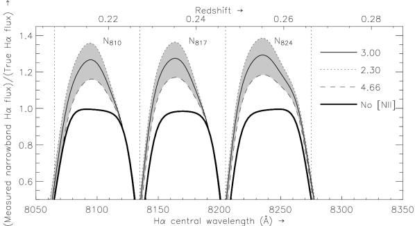
Figure 10: Measured narrowband H$\alpha$ flux in each WFILAS filter as a function of redshift, expressed as a fraction of the true H$\alpha$ flux. The thick solid line shows the measured H$\alpha$ flux in the absence of [N ii] and approximately traces the filter transmission curve. The shaded envelope shows the effect of the [N ii] line over the range H$\alpha$/[N ii]_tot = 2.30 (dotted) to 4.66 (dashed), centred on 3.00 (thin solid line). The vertical dotted lines indicate where the filter transmission is 50 %.

$\frac{{\mathrm{H\alpha}}{}}{{\mbox{{[\sc N\,ii]}}}{}_{\mathrm{tot}}}$	Reference	$\log\frac{{\mbox{{[\sc N\,ii]}}}{}}{{\mathrm{H\alpha}}{}}$	$\frac{\mathrm{{\mathrm{H\alpha}}{}(narrowband)}}{\mathrm{{\mathrm{H\alpha}}{}(true)}}$
			New A	$N_{817}$	$N_{824}$
2.30	Pascual et al. (2007)	$-0.49$	1.04	1.04	1.14
3.00	this paper	$-0.60$	0.99	0.99	1.08
4.66	Ly et al. (2007)	$-0.79$	0.93	0.93	1.00

Table 6: Ratio of H$\alpha$ to combined [N ii] line flux for a range of values in the literature (as indicated). The third column shows the corresponding values of log of the ratio of the [N ii] $\lambda$6585 to H$\alpha$ line flux. The last three columns indicate the mean ratio of the H$\alpha$ flux measured in the narrowband filters to the true flux where the filter transmission is $\geq$ 50 %.

The filters used in this survey are sufficiently narrow (FWHM$=70$ Å) that the forbidden lines of [N ii] $\lambda\lambda$6550,6585 can affect the measurement of H$\alpha$ flux through narrowband imaging. The proximity of lines complicates the estimate of H$\alpha$ line flux in two ways. In the case where H$\alpha$ is central to the filter, both [N ii] lines contribute to the narrowband-derived flux attributed to the H$\alpha$ flux. In the case where H$\alpha$ is near the filter edge, then an [N ii] line is either lost to an adjacent filter (where it contributes to the measured continuum) or lost to the filters altogether. Due to the finite width of emission lines and the steepness of the filters, this is a gradual transition.

We have calculated the H$\alpha$ flux as measured from the narrowband imaging and compared it to its true value over a range of galaxy redshifts, taking into account our filter setup. This was done by taking the spectrum of one of our galaxies and fitting the H$\alpha$ line, as well as the [N ii]- and [S ii] doublets. We then convolved the fit with each of our filter profiles and calculated the line flux from the filters in the same way as for the survey. A range of different values of H$\alpha$/[N ii]_tot have been used, since this ratio depends on metallicity (e.g. Osterbrock, 1989; Kewley et al., 2001; Kauffmann et al., 2003). We have used two extreme values 2.30 by Pascual et al., 2007 and 4.66 by Ly et al., 2007 to reflect the wide range of metallicities found in these galaxies. A third value of 3.00 was measured from a high quality spectrum used for emission line fitting.

The results are shown in Figure 10. Average values of the ratio of measured to true H$\alpha$ flux are indicated in Table 6. The narrowband H$\alpha$ flux overestimates the true flux by about 10 % when averaged over all redshifts pertaining to a specific filter. However, the ratio can peak around 40 % in the innermost 15 % of filter coverage. This peak corresponds to the specific case of an idealised square filter containing all three lines as calculated by Pascual et al. (2007). This is a worse case scenario that only occurs rarely in practise. In the vast majority of cases the effect of [N ii] is moderated by the sloping edges of a real filter profile, or complete absence of [N ii] from the narrowband filters altogether. Given the 70 Å width of our filters and the $\sim 50$ Å width of the H$\alpha$/[N ii] group, the chance of having all three lines in the same filter is uncommon.

As the overall effect of [N ii] is approximately 10 % (corresponding to 0.04 in $\log L$), we do not make any correction for it.

4.4.2 AGN contribution

The presence of an active nucleus in a galaxy can contribute H$\alpha$ line flux in addition to that due to normal star formation. For example, Pascual et al. (2001) have found approximately 15 % of their luminosity density to be due to galaxies identified as AGNs. We computed the fraction of H$\alpha$ contribution due to AGN in our sample using the line diagnostic relations as determined by Kewley et al. (2001) and Kauffmann et al. (2003). We selected galaxies from both fields where the fluxes of the emission lines H$\beta$, [Oiii] $\lambda$5007 and [N ii] $\lambda$6585 have been measured with a signal-to-noise ratio $\geq 2$. The line ratios and the line diagnostic relations are indicated in the Baldwin-Phillips-Terlevich (BPT; Baldwin et al., 1981) diagram of Figure 11.

Two of the galaxies lie above the extreme starburst demarcation of Kewley et al. (2001, solid line) and have $\log({\mbox{{[\sc N\,ii]}}}{}/{\mathrm{H\alpha}}{})\geq-0.6$, which classifies them as AGNs. A third galaxy, also with $\log({\mbox{{[\sc N\,ii]}}}{}/{\mathrm{H\alpha}}{})\geq-0.6$, lies below this demarcation, but above the pure star formation boundary of Kauffmann et al. (2003, dashed line), making this galaxy a composite case.

If we consider the total H$\alpha$ contribution from the two AGNs in it amounts to 5 % of the total H$\alpha$ flux from this subsample. Overall, this AGN contribution would result in a decrease in the star formation density of $\log\dot{\rho}=0.02$. If we include the composite galaxy as a third AGN, the decrease is $\log\dot{\rho}=0.04$.

Figure 11: BPT diagram for 35 galaxies where the fluxes of the emission lines H$\beta$, [Oiii] $\lambda$5007 and [N ii] $\lambda$6585 have been measured with a signal-to-noise ratio $\geq 2$. Indicated by the solid line is the extreme starburst demarcation of Kewley et al. (2001) and the dashed line the demarcation of pure star formation of Kauffmann et al. (2003). The vertical line is drawn at $\log({\mbox{{[\sc N\,ii]}}}{}/{\mathrm{H\alpha}}{})=-0.6$. The median uncertainty is indicated by the error bars. The galaxies indicated by the open circles lie above the Kewley et al. (2001) line and are most likely influenced by AGN activity. A third galaxy, marked by an open square, lies within the two demarcations and is a composite source. The remaining galaxies, shown by the closed circles, lie below the Kauffmann et al. (2003) relation and left of the $\log({\mbox{{[\sc N\,ii]}}}{}/{\mathrm{H\alpha}}{})=-0.6$ line and are pure star forming galaxies.

4.4.3 [S ii] contribution

CDFS				S11
$\alpha$	$\log L^{*}$	$\log\phi^{*}$		$\alpha$	$\log L^{*}$	$\log\phi^{*}$
$-$1.01 $\pm$ 0.32	41.28 $\pm$ 0.15	$-$1.88 $\pm$ 0.19		$-$1.17 $\pm$ 0.50	41.23 $\pm$ 0.24	$-$2.24 $\pm$ 0.34
$\left(\begin{array}[]{rrr}1.00000&-0.91849&0.95680\\ -0.91849&1.00000&-0.96615\\ 0.95680&-0.96615&1.00000\end{array}\right)$				$\left(\begin{array}[]{rrr}1.00000&-0.90882&0.95080\\ -0.90882&1.00000&-0.97085\\ 0.95080&-0.97085&1.00000\end{array}\right)$

Table 7: Schechter parameters for the H$\alpha$ luminosity functions where the [S ii] galaxies at $z\sim 0.21$ are assumed to be H$\alpha$ galaxies at $z\sim 0.24$. They were determined using a Levenberg-Marquardt $\chi^{2}$ minimisation. The correlation matrices $\rho_{ij}$ for each are shown below.

Surveys that only apply colour criteria to determine the nature of the emission line are unable to distinguish between H$\alpha$ emitters at $z\sim 0.24$ and [S ii] emitters at $z\sim 0.21$ (Section 3.1 and Figure 2). The previous calculations of the H$\alpha$ fraction assume that it is possible to distinguish between H$\alpha$ and [S ii] emitters. Since this can only be done with spectroscopy, we have also derived the H$\alpha$ luminosity function for the case where [S ii] emitters are taken to be H$\alpha$ emitters. This gives an indication of the impact of having sole reliance on colour criteria and no spectroscopic follow up. Figure 12 shows the difference between H$\alpha$ luminosity functions for the CDFS and S11 fields where the [S ii] galaxies were assumed to be H$\alpha$. The Schechter parameters that belong to the alternative Schechter functions are given in Table 7.

The star formation density as determined from these hypothetical [S ii]-as-H$\alpha$ luminosity functions down to our survey limit are $\log\dot{\rho}(L>L_{\mathrm{lim}})=-2.22^{+0.10}_{-0.13}$ and $-1.81^{+0.070}_{-0.083}$ for the S11 and CDFS fields, respectively. In the S11 field there were only a handful of galaxies (4) identified at $z\sim 0.21$, while the CDFS contained a significant number (30). Hence the results of the CDFS field are more significantly affected and an increase in the star formation density $\log\dot{\rho}$ in this field of 0.12 (about 30 %) can be seen. This exercise demonstrates how a foreground overdensity of [S ii] emitters, if present, can significantly influence the H$\alpha$ star formation density. For this reason, it is imperative to have at least some spectroscopic follow up to a narrowband survey to make such situations obvious.

Figure 12: Differences between our derived H$\alpha$ luminosity distribution (Figure 7) and that assuming all [S ii] galaxies at $z\sim 0.21$ to be H$\alpha$. The values for the Schechter parameters to the luminosity diagram including the [S ii] galaxies are indicated in Table 7.

5 Environmental properties

The suppression of star formation rates at the centres of clusters has been well established both through direct observation (Lewis et al., 2002; Balogh et al., 1997, 1998; Kodama et al., 2001, 2004; Gómez et al., 2003), as well as a changing mix of morphological types (Dressler, 1980). Such high density environments provide a range of dynamical mechanisms whereby galaxy encounters rapidly strip gas from any potential star forming galaxies (e.g. Couch et al., 2001, and references therein). Recent observations have suggested a continuation of this trend across structures at larger scales and lower density enhancements than clusters (Gómez et al., 2003; Gray et al., 2004). Accordingly we examine our two fields for evidence of star formation rates that are driven by either the general galaxy environment, or alternatively, the local distribution of star forming galaxies.

Usually, the amount of galaxy clustering is expressed as a function of projected density

$$\Sigma_{n}=\frac{n}{\pi r_{n}^{2}}~{},$$ (10)

where $r_{n}$ (in Mpc) is the distance to the $n$th (usually $n=10$) nearest neighbouring galaxy with $M_{B}<-19$. In cluster environments the star formation rate has been observed to be quenched at galaxy densities above 1 Mpc^-2 (Lewis et al., 2002; Gómez et al., 2003).

Figure 13: (a) The mean and median star formation rate per galaxy (in M_⊙ yr^-1) and the fraction of galaxies with a star formation rate $>1$ M_⊙ yr^-1 as a function of the projected density $\Sigma_{10}$ of ordinary galaxies (taken from the COMBO-17 survey). The errorbars in the two top panels are the jackknife estimates of the standard error, while in the bottom panel they are standard deviations. The small crosses indicate the values for each individual star forming galaxy. The thick lines in the middle panel indicate the 25th and 75th percentile for each bin. The numbers in the bottom panel indicate the number of galaxies included in each point. Some of the individual galaxies have values outside the range of star formation rates plotted and hence are not indicated. (b) Same as (a), but as a function of star forming galaxy density $\Sigma^{*}_{3}$.

In Figure 13(a) we show the fraction of galaxies with a star formation rate exceeding 1 M_⊙ yr^-1, as well as median and mean star formation rate per galaxy as a function of the projected density of the general galaxy population. This uses data for all of the spectroscopically confirmed star forming galaxies at $z\sim 0.24$ for both of our fields combined. The indicated errorbars in the two top panels were determined using the jackknife estimator, while in the bottom panel they are the standard deviation. We also show the 25th and 75th percentile values for each bin in the middle panel. We determined the projected density by using the usual $r_{10}$ measure of the tenth-nearest star forming galaxy to each ordinary galaxy. Ordinary galaxies were taken from the photometric redshift catalogues of the COMBO-17 survey (Wolf et al., 2003, K. Meisenheimer, priv. comm.) as galaxies with $B_{AB}<22$ (corresponding to $M_{B}=-19$) between $0.21\leq z\leq 0.29$. As the thickness of the redshift slice influences the value of projected density, we scale it using the difference in the thickness of the redshift slice of our survey and the average thickness of the $3\sigma$ cluster volumes (where $\sigma$ is the velocity dispersion of the cluster) used in Lewis et al. (2002).

Since we did not target any known clusters with our fields, we expect that there will be little or no evidence for star formation suppression in our fields. Typically, the projected density for galaxies within the virial radius of a cluster is $\sim 4$ Mpc^-2 and at the centre of some rich clusters can be as high as $10$ Mpc^-2 (Lewis et al., 2002). Indeed, as Figure 13(a) shows, there is negligible change in the star formation rate per unit density for the galaxies in both our fields (noting that the highest density point is affected by poor number statistics). Furthermore, we confirm levels of star formation that are typical for the range of typical field galaxy densities probed by our data as found by previous surveys (e.g. Lewis et al., 2002; Gómez et al., 2003). Generally, the distribution of star formation rates in a given density bin is rather asymmetric, making the median a more reliable measure than the mean.

In Figure 13(b) we show the same measures as for (a), but as a function of projected density of the spectroscopically confirmed star forming galaxies at $0.23\leq z\leq 0.26$. There are roughly one-third as many star forming galaxies as not, and so we redefine the projected density in terms of distance to the third-nearest galaxy, $\Sigma^{*}_{3}$. As a consequence, $\Sigma^{*}_{3}$ and $\Sigma_{10}$ span a similar range of density values. We observe in Figure 13(b) that star formation per galaxy increases with increasing density. Noting again that the highest density bin is affected by poor number statistics. Although not conclusive, this is consistent with galaxy evolution scenarios that see galaxy-galaxy interactions as triggers for bursts of star formation (Alonso et al., 2004; Perez et al., 2006).

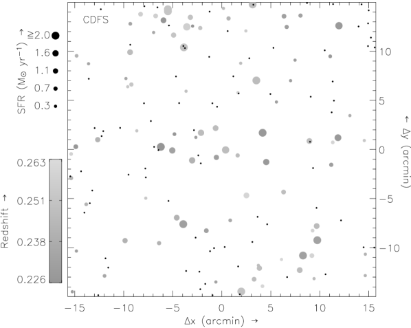
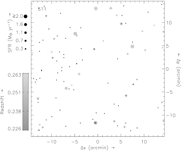
Figure 14: Spatial distribution of the spectrally confirmed H$\alpha$ galaxies in both our fields (solid circles). The size of the circles indicates the star formation rate of the galaxy derived from the narrowband flux and the grey-scale the redshift. The black dots are galaxies that have not been spectroscopically confirmed yet and have a colour $0.5\leq(B-R){}\leq 1.3$, which corresponds to the colour interval of our confirmed H$\alpha$ galaxies (Figure 2).

To examine the apparent relationship between star formation rate and projected density of star forming galaxies, we plot the spatial distribution of our spectrally confirmed H$\alpha$ galaxies in Figure 14. The size of the points indicates their star formation rate and their shade of grey the redshift. Probable (but unconfirmed) H$\alpha$ candidates are also shown. These were selected on the basis of colour ($0.5\leq(B-R){}\leq 1.3$; see Figure 2) and having either indeterminate or non-existent spectra.

The distribution of star forming galaxies in the CDFS field (Figure 13b) suggests a tendency for grouping of the star forming galaxies. However, the eye is remarkably good at making out patterns in noisy distributions and thus we should be cautious in these interpretations (e.g. p35 of Peebles, 1993). On the other hand, the distribution of star forming galaxies at $z\sim 0.24$ in the S11 field (Figure 14) is apparently less structured than the CDFS. Because of this, we infer that the trend of increasing star formation with rising density of star forming galaxies is largely attributable to the data from the CDFS field. This contrast between the fields can also be seen in differences in the H$\alpha$ space-densities given by the two luminosity functions in Figure 7. As a consequence, the star formation density of the S11 field is lower than that of the CDFS (Figure 8). This is due to the lower H$\alpha$ fraction in the S11 field compared to the CDFS field (Figure 5), to the extend that can be seen given the more limited spectroscopy on the former.

A more robust approach would be the derivation of two-point correlation statistics of the star forming galaxies, which could directly test for clustering tendencies in the CDFS field compared to S11. Such analyses are beyond the scope of this paper, but will be addressed in a future work.

6 Summary and conclusions

In this paper we report the results of a survey for H$\alpha$ emitting galaxies at $z\sim 0.24$. We used two fields from the Wide Field Imager Lyman Alpha Search (WFILAS). It consists of imaging in three narrowband filters (FWHM $=70$ Å), an encompassing intermediate band filter (FWHM $=220$ Å), supplemented with broadband $B$ and $R$. The narrowband filters cover a redshift range of $0.23\lesssim z\lesssim 0.26$ for H$\alpha$ galaxies. These galaxies were selected by having an excess flux in one of the narrowband over to the other two, while also being detected in the intermediate and broadband $R$ filters. This yielded a total of 707 candidate emission line galaxies (after the removal of stellar contaminants) for both fields.

Of the 372 and 335 candidates, we observed 301 and 255 through spectroscopic follow-up for the CDFS and S11 fields, respectively. We have identified emission in 189 and 117 candidates and confirmed that around half of these galaxies are H$\alpha$ at $z\sim 0.24$. A significant number of galaxies were also found at $z\sim 0.21$ by means of their [S ii] emission. Other galaxies found were [Oii] and H$\beta$/[Oiii] emitters at $z\sim 1.2$ and $z\sim 0.6-0.7$, respectively. Through use of the spectroscopy, we refined our colour selection to account for galaxies with a single emission line, leading to a measure of the fraction of H$\alpha$ galaxies as a function of narrowband flux in both of these regions of the sky. We also used the spectroscopy to determine a generic extinction correction using the Balmer decrement.

We have determined the H$\alpha$ luminosity function at $z\sim 0.24$ separately for both of our fields after correcting for imaging and spectroscopic incompleteness, extinction and contamination from interlopers. We find small differences in their slope and turn-over luminosity while their normalisations were the same. When compared to recent H$\alpha$ surveys, there is remarkable agreement between the luminosity function of our CDFS field with that one the Fabry-Perot imaging survey of Hippelein et al. (2003). Differences between our fields were of the order expected by cosmic variance but less than the scatter between the H$\alpha$ luminosity functions of recent surveys. We surmise that while cosmic variance is a major contributor to this scatter, it is differences in methodology between surveys (mainly differences in selection criteria) that dominate discrepancies between H$\alpha$ luminosity functions and its related observables at $z\sim 0.24$. A survey that covers $10-20\times$ the volume of one of our fields is required to get the uncertainty due to cosmic variance to the levels of Gallego et al. (1995).

We estimated the star formation density for both our fields to be $\log\dot{\rho}=-1.93^{+0.08}_{-0.10}$ and $-2.24^{+0.11}_{-0.14}$ ($\dot{\rho}$ in M_⊙ yr^-1) for the CDFS and S11 fields, respectively, down to our survey limit of $\log F_{\mathrm{line}}=-16.0$ ($F_{\mathrm{line}}$ in erg s^-1 cm^-2) or $\log L_{\mathrm{line}}=40.6$ ($L_{\mathrm{line}}$ in erg s^-1). These values are comparable to other surveys at this redshift when calculated to the same flux limit. Correcting for AGN would decrease these values by 0.02 to 0.04 depending on exactly how much of the H$\alpha$ flux is contributed by the active nucleus rather than by normal star formation.

Furthermore, we determined the star formation density in the hypothetical case where [S ii] emitters at $z\sim 0.21$ were classified as H$\alpha$ to illustrate the problems associated with solely relying colour selections. The star formation density $\log\dot{\rho}$ of the S11 field does not change by much (+0.02). On the other hand, the star formation density in the CDFS increases by 0.12, due to the large number of foreground [S ii] galaxies at $z\sim 0.21$.

We explored the amount of star formation with respect to the local environment and found that the star formation rates were typical for the field galaxy densities probed, in agreement with the results of previous work. However, we also found tentative evidence of an increase in star formation rate per galaxy with increasing density of the star forming galaxies. This supports scenarios where merger events are triggers for enhanced star formation, provided it can be demonstrated to be occurring on the smallest scales. We explored this trend by examining the spatial distribution of our fields individually and found that it was largely attributable to one field. A formal study of the clustering statistics of this field is required to confirm this and will be the subject of a future study.

References

- Ajiki et al. (2003) Ajiki M., Taniguchi Y., Fujita S. S., Shioya Y., Nagao T., Murayama T., Yamada S., Umeda K., Komiyama Y., 2003, AJ, 126, 2091
- Alonso et al. (2004) Alonso M. S., Tissera P. B., Coldwell G., Lambas D. G., 2004, MNRAS, 352, 1081
- Baldry & Glazebrook (2003) Baldry I. K., Glazebrook K., 2003, ApJ, 593, 258
- Baldwin et al. (1981) Baldwin J. A., Phillips M. M., Terlevich R., 1981, PASP, 93, 5
- Balogh et al. (1997) Balogh M. L., Morris S. L., Yee H. K. C., Carlberg R. G., Ellingson E., 1997, ApJ, 488, L75+
- Balogh et al. (1998) Balogh M. L., Schade D., Morris S. L., Yee H. K. C., Carlberg R. G., Ellingson E., 1998, ApJ, 504, L75+
- Bertin & Arnouts (1996) Bertin E., Arnouts S., 1996, A&AS, 117, 393
- Bessell (1999) Bessell M. S., 1999, PASP, 111, 1426
- Bruzual & Charlot (2003) Bruzual G., Charlot S., 2003, MNRAS, 344, 1000
- Calzetti (2001) Calzetti D., 2001, PASP, 113, 1449
- Calzetti et al. (2000) Calzetti D., Armus L., Bohlin R. C., Kinney A. L., Koornneef J., Storchi-Bergmann T., 2000, ApJ, 533, 682
- Cardelli et al. (1989) Cardelli J. A., Clayton G. C., Mathis J. S., 1989, ApJ, 345, 245
- Cole et al. (2001) Cole S., Norberg P., Baugh C. M., Frenk C. S., Bland-Hawthorn J., Bridges T., Cannon R., Colless M., Collins C., Couch W., Cross N., Dalton G., De Propris R., Driver S. P., Efstathiou G., et al. 2001, MNRAS, 326, 255
- Condon (1992) Condon J. J., 1992, ARA&A, 30, 575
- Couch et al. (2001) Couch W. J., Balogh M. L., Bower R. G., Smail I., Glazebrook K., Taylor M., 2001, ApJ, 549, 820
- Cowan (1998) Cowan G., 1998, Statistical data analysis. Oxford University Press
- Cowie et al. (1996) Cowie L. L., Songaila A., Hu E. M., Cohen J. G., 1996, AJ, 112, 839
- Daigne et al. (2006) Daigne F., Olive K. A., Silk J., Stoehr F., Vangioni E., 2006, ApJ, 647, 773
- Doherty et al. (2006) Doherty M., Bunker A., Sharp R., Dalton G., Parry I., Lewis I., 2006, MNRAS, 370, 331
- Dressler (1980) Dressler A., 1980, ApJ, 236, 351
- Efron & Gong (1983) Efron B., Gong G., 1983, The American Statistician, 37, 36
- Fardal et al. (2006) Fardal M. A., Katz N., Weinberg D. H., Dav’e R., 2006, astro-ph/0604534
- Fujita et al. (2003) Fujita S. S., Ajiki M., Shioya Y., Nagao T., Murayama T., Taniguchi Y., Umeda K., Yamada S., Yagi M., Okamura S., Komiyama Y., 2003, ApJ, 586, L115
- Gal-Yam & Maoz (2004) Gal-Yam A., Maoz D., 2004, MNRAS, 347, 942
- Gallego et al. (2002) Gallego J., García-Dabó C. E., Zamorano J., Aragón-Salamanca A., Rego M., 2002, ApJ, 570, L1
- Gallego et al. (1995) Gallego J., Zamorano J., Aragon-Salamanca A., Rego M., 1995, ApJ, 455, L1+
- Gawiser et al. (2006) Gawiser E., van Dokkum P. G., Gronwall C., Ciardullo R., Blanc G. A., Castander F. J., Feldmeier J., Francke H., Franx M., Haberzettl L., Herrera D., Hickey T., Infante L., Lira P., et al. 2006, ApJ, 642, L13
- Glazebrook et al. (1999) Glazebrook K., Blake C., Economou F., Lilly S., Colless M., 1999, MNRAS, 306, 843
- Gómez et al. (2003) Gómez P. L., Nichol R. C., Miller C. J., Balogh M. L., Goto T., Zabludoff A. I., Romer A. K., Bernardi M., Sheth R., Hopkins A. M., Castander F. J., Connolly A. J., Schneider D. P., Brinkmann J., Lamb D. Q., SubbaRao M., York D. G., 2003, ApJ, 584, 210
- Gray et al. (2004) Gray M. E., Wolf C., Meisenheimer K., Taylor A., Dye S., Borch A., Kleinheinrich M., 2004, MNRAS, 347, L73
- Heavens et al. (2004) Heavens A., Panter B., Jimenez R., Dunlop J., 2004, Nature, 428, 625
- Hippelein et al. (2003) Hippelein H., Maier C., Meisenheimer K., Wolf C., Fried J. W., von Kuhlmann B., Kümmel M., Phleps S., Röser H.-J., 2003, A&A, 402, 65
- Hopkins (2004) Hopkins A. M., 2004, ApJ, 615, 209
- Hopkins & Beacom (2006) Hopkins A. M., Beacom J. F., 2006, ApJ, 651, 142
- Hopkins et al. (2003) Hopkins A. M., Miller C. J., Nichol R. C., Connolly A. J., Bernardi M., Gómez P. L., Goto T., Tremonti C. A., Brinkmann J., Ivezić Ž., Lamb D. Q., 2003, ApJ, 599, 971
- Hu et al. (2004) Hu E. M., Cowie L. L., Capak P., McMahon R. G., Hayashino T., Komiyama Y., 2004, AJ, 127, 563
- Jansen et al. (2001) Jansen R. A., Franx M., Fabricant D., 2001, ApJ, 551, 825
- Jones & Bland-Hawthorn (2001) Jones D. H., Bland-Hawthorn J., 2001, ApJ, 550, 593
- Jones et al. (2006) Jones D. H., Peterson B. A., Colless M., Saunders W., 2006, MNRAS, 369, 25
- Jones et al. (2004) Jones D. H., Saunders W., Colless M., Read M. A., Parker Q. A., Watson F. G., Campbell L. A., Burkey D., Mauch T., Moore L., Hartley M., Cass P., James D., Russell K., Fiegert K., Dawe J., Huchra J., Jarrett T., Lahav O., et al. 2004, MNRAS, 355, 747
- Juneau et al. (2005) Juneau S., Glazebrook K., Crampton D., McCarthy P. J., Savaglio S., Abraham R., Carlberg R. G., Chen H.-W., Le Borgne D., Marzke R. O., Roth K., Jørgensen I., Hook I., Murowinski R., 2005, ApJ, 619, L135
- Kauffmann et al. (2003) Kauffmann G., Heckman T. M., Tremonti C., Brinchmann J., Charlot S., White S. D. M., Ridgway S. E., Brinkmann J., Fukugita M., Hall P. B., Ivezić Ž., Richards G. T., Schneider D. P., 2003, MNRAS, 346, 1055
- Kennicutt (1992) Kennicutt Jr. R. C., 1992, ApJ, 388, 310
- Kennicutt (1998) Kennicutt Jr. R. C., 1998, ARA&A, 36, 189
- Kewley et al. (2001) Kewley L. J., Dopita M. A., Sutherland R. S., Heisler C. A., Trevena J., 2001, ApJ, 556, 121
- Kewley et al. (2004) Kewley L. J., Geller M. J., Jansen R. A., 2004, AJ, 127, 2002
- Kodama et al. (2004) Kodama T., Balogh M. L., Smail I., Bower R. G., Nakata F., 2004, MNRAS, 354, 1103
- Kodama et al. (2001) Kodama T., Smail I., Nakata F., Okamura S., Bower R. G., 2001, ApJ, 562, L9
- Lewis et al. (2002) Lewis I., Balogh M., De Propris R., Couch W., Bower R., Offer A., Bland-Hawthorn J., Baldry I. K., Baugh C., Bridges T., Cannon R., Cole S., Colless M., Collins C., Cross N., Dalton G., et al. 2002, MNRAS, 334, 673
- Lewis et al. (2002) Lewis I. J., Cannon R. D., Taylor K., Glazebrook K., Bailey J. A., Baldry I. K., Barton J. R., Bridges T. J., Dalton G. B., Farrell T. J., Gray P. M., Lankshear A., McCowage C., Parry I. R., Sharples R. M., Shortridge K., Smith G. A., et al. 2002, MNRAS, 333, 279
- Lilly et al. (1996) Lilly S. J., Le Fevre O., Hammer F., Crampton D., 1996, ApJ, 460, L1+
- Ly et al. (2007) Ly C., Malkan M. A., Kashikawa N., Shimasaku K., Doi M., Nagao T., Iye M., Kodama T., Morokuma T., Motohara K., 2007, ApJ, 657, 738
- Madau et al. (1996) Madau P., Ferguson H. C., Dickinson M. E., Giavalisco M., Steidel C. C., Fruchter A., 1996, MNRAS, 283, 1388
- Madgwick et al. (2002) Madgwick D. S., Lahav O., Baldry I. K., Baugh C. M., Bland-Hawthorn J., Bridges T., Cannon R., Cole S., Colless M., Collins C., Couch W., Dalton G., De Propris R., Driver S. P., Efstathiou G., et al. 2002, MNRAS, 333, 133
- Massarotti et al. (2001) Massarotti M., Iovino A., Buzzoni A., 2001, ApJ, 559, L105
- Mendoza (1983) Mendoza C., 1983, in Flower D. R., ed., Planetary Nebulae Vol. 103 of IAU Symposium, Recent advances in atomic calculations and experiments of interest in the study of planetary nebulae. pp 143–172
- Miszalski et al. (2006) Miszalski B., Shortridge K., Saunders W., Parker Q. A., Croom S. M., 2006, MNRAS, 371, 1537
- Oke & Gunn (1983) Oke J. B., Gunn J. E., 1983, ApJ, 266, 713
- Osterbrock (1989) Osterbrock D. E., 1989, Astrophysics of gaseous nebulae and active galactic nuclei. Research supported by the University of California, John Simon Guggenheim Memorial Foundation, University of Minnesota, et al. Mill Valley, CA, University Science Books, 1989, 422 p.
- Panter et al. (2003) Panter B., Heavens A. F., Jimenez R., 2003, MNRAS, 343, 1145
- Pascual et al. (2001) Pascual S., Gallego J., Aragón-Salamanca A., Zamorano J., 2001, A&A, 379, 798
- Pascual et al. (2007) Pascual S., Gallego J., Zamorano J., 2007, PASP, 119, 30
- Peebles (1993) Peebles P. J. E., 1993, Principles of physical cosmology. Princeton Series in Physics, Princeton, NJ: Princeton University Press, —c1993
- Pei & Fall (1995) Pei Y. C., Fall S. M., 1995, ApJ, 454, 69
- Pei et al. (1999) Pei Y. C., Fall S. M., Hauser M. G., 1999, ApJ, 522, 604
- Perez et al. (2006) Perez M. J., Tissera P. B., Lambas D. G., Scannapieco C., 2006, A&A, 449, 23