Detection of Spin Correlations in Optical Lattices by Light Scattering

Abstract

We show that spin correlations of atoms in an optical lattice can be reconstructed by coupling the system to the light, and by measuring correlations between the emitted photons. This principle is the basis for a method to characterize states in quantum computation and simulation with optical lattices. As examples, we study the detection of spin correlations in a quantum magnetic phase, and the characterization of cluster states.

Ultracold atoms in optical lattices open exciting prospects for the investigation of quantum many–body phases in a highly controllable setup. For example, spin–spin interactions between atoms in a Mott insulator state can be tuned in such a way that one can simulate a rich variety of models from quantum magnetism DDL . Furthermore, this system is ideally suited to implement a quantum register for quantum computation DJ98 , and to realize multiparticle entangled states with cold controlled collisions BCJD99 ; JBCGZ99 . An important benchmark in this direction has been the creation of a cluster state MGWRHB03 , since it can be used as a resource for measurement based universal quantum computation RB01 ; RBB03 .

A major disadvantage of this setup is the fact that atoms are separated by optical wavelengths, and thus it is difficult to address them individually. This impedes one to measure directly the spatial dependence of spin–spin correlations, which is essential in the characterization of quantum phases. For these reasons the development of accurate methods to measure properties of atomic operators is basic to the usefulness of optical lattices for quantum computation and simulation. A possible solution relies on the detection of the atom number distribution in time of flight (TOF) imaging. Within this technique atomic density operators in momentum space are measured by taking absorption images of the expanding cloud, after having switched off the trapping potentials. From TOF images density–density correlation functions in momentum space ADL04 ; FGWMGB05 ; GRSJ05 are reconstructed by detecting statistical correlations between different images. On the other hand, one may use quantum non-demolition techniques on the atom–light interaction in order to determine certain atomic collective observables EZS07 ; ERRLPA07 .

In this letter we describe an alternative approach which allows one to measure spin correlations without switching off the optical potential. Furthermore, it is not necessary to drive the atoms out of the strongly correlated regime, thus avoiding certain complications that are met in TOF measurements of interacting fermions. Our method is based on off–resonant scattering of an incident laser with the trapped atoms. Scattered photons with a certain polarization are coupled to certain spin operators. In that way correlations between photons emitted in different directions are proportional to ground state correlations of spin operators in momentum space. Different detection schemes, such as photon counting or homodyne detection, may give information of different types of correlations. One of the strengths of the method is that it is based on photon detection, and not on atom detection. For this reason, detection of any possible spin–spin correlation is achieved here naturally, just by controlling the polarization of the lasers and of the detected photons. The correlation of an arbitrary number of spin operators can be achieved by considering correlations of different detections.

We consider an optical lattice filled with $N$ atoms in a Mott insulator state with at most one atom per site. Each atom carries an arbitrary ground state hyperfine spin $J$, and has an optical dipole transition of frequency $\omega_{0}$ to an excited states manifold of spin $J^{\prime}$. This transition is coupled with an off–resonant laser of frequency $\omega_{L}$, wavevector ${\bf k}_{L}$, and a certain linear polarization $\sigma_{L}$. Photons are then scattered with momentum ${\bf k}$ and two different polarizations $\beta$, such that $\beta\neq\sigma_{L}$. Light modes with momentum ${\bf k}$ are coupled to atomic operators $J^{\Delta{\bf k}}_{\beta}=1/\sqrt{N}\sum_{j}J_{\beta}^{j}e^{i{\Delta{\bf k}}\cdot{\bf r}_{j}}$, with $\Delta{\bf k}={\bf k}-{\bf k}_{L}$, where $J_{\beta}^{j}$ are atomic spin operators, and the vector ${\bf r}_{j}$ denotes the position of the atoms in the lattice. This allows us to describe correlations of spin operators with different momentum, which as it will be later discussed provides us in principle with full information to reconstruct spin correlations in the position space. We present the following results: (i) By measuring correlations between photons with momenta ${\bf k}$ we reconstruct correlations between atomic spin operators $J^{\Delta{\bf k}}_{\beta}$, such that $k=k_{\textmd{L}}$. Full access to correlations both in momentum and position space requires that $k_{L}r_{0}>\sqrt{2}\pi$ ($\sqrt{3}\pi$) in $2D$ ($3D$) square lattices, where $r_{0}$ is the lattice constant. However, these conditions are not always necessary to characterize a state in the momentum space. (ii) Measured correlations are in the ground state provided that the measurement time $T\ll 1/\Gamma$, where $\Gamma$ is the spontaneous emission rate. The validity of this approximation is studied by simulating the emission properties of interacting atoms in a lattice by means of a bosonic description of spin excitations. (iii) As an illustration of applications, we discuss the measurement of a magnetic phase, an example that is relevant to quantum simulation, as well as a measurement of a cluster state in a $2D$ lattice, which has an important application in quantum computation.

The incident laser has a large detuning $\Delta=\omega_{J^{\prime}}-\omega_{L}$, with respect to the uppermost level of $J^{\prime}$, with frequency $\omega_{J^{\prime}}$. In that situation, the excited manifold can be adiabatically eliminated K05 ; J03 , and the evolution of any operator $A$ acting on the spin $J$ manifold, can be written in terms of an effective Hamiltonian for light–matter interaction $(d/dt)A=i/\hbar[H^{\textmd{eff}}_{\textmd{lm}},A]$. Along the same lines as in K05 ; J03 ; EZS07 , the effective Hamiltonian can be written as

$$H^{\textmd{eff}}_{\textmd{lm}}=ig\sum_{j}\left({\bf E}_{\textmd{tot}}^{j\dagger}\cdot({\bf J}_{j}\times{\bf E}_{\textmd{tot}}^{j})+h.c.\right),$$ (1)

where $g=d^{2}a_{1}/\Delta$, $d$ is the atomic dipole matrix element, and $a_{1}$ is a constant that depends on the particular transition considered. The electromagnetic field is usually expressed in terms of the two orthonormal polarization vectors $\hat{\bf e}_{{\bf k}l}\bot{\bf k}$ ($l=1,2$) and the corresponding creation (annihilation) operators $a^{\dagger}_{{\bf k}l}$ ($a_{{\bf k}l}$). Nevertheless, it is more convenient for us to express ${\bf E}_{\textmd{tot}}^{j}$ in the laboratory frame. We decompose the field in the following way: ${\bf E}_{\textmd{tot}}^{j}=\sum_{\sigma}(\widetilde{{\bf E}}_{\sigma}^{j-}+\widehat{{\bf E}}_{\sigma}^{j+}+{\bf E}^{j+}_{L})$, where $\widetilde{{\bf E}}_{\sigma}^{j+}=\sum_{{\bf k}}\epsilon_{{\bf k}}a_{{\bf k}\sigma}e^{-i\Delta^{+}_{k}t+i{\bf k}\cdot{\bf r}_{j}}\hat{\bf\sigma}$, and $\widehat{{\bf E}}_{\sigma}^{j+}=\sum_{{\bf k}}\epsilon_{{\bf k}}a_{{\bf k}\sigma}e^{-i\Delta^{-}_{k}t+i{\bf k}\cdot{\bf r}_{j}}\hat{\bf\sigma}$ are fast and slowly rotating terms respectively rot , and ${\bf E}^{j+}_{L}=\epsilon_{L}e^{-i{\bf k}_{L}\cdot{\bf r}_{j}}{\hat{\bf\sigma}}_{L}$ is the laser field. The constants are $\epsilon_{k}=\sqrt{\hbar\omega_{k}/(2\epsilon_{0}\upsilon)}$, $\Delta^{\pm}_{k}=\omega_{k}\pm\omega_{L}$, and ${\sigma}_{L},\sigma=x,y,z$. In addition, we have defined photon operators in the laboratory frame, $a_{{\bf k}x}=\cos\theta\cos\phi a_{{\bf k}1}+\sin\phi a_{{\bf k}2}$, $a_{{\bf k}y}=\cos\theta\sin\phi a_{{\bf k}1}-\cos\phi a_{{\bf k}2}$ and $a_{{\bf k}z}=-\sin\theta a_{{\bf k}1}$, with $\theta$ and $\phi$ the angular coordinates of the wave vector ${\bf k}$ in the laboratory frame.

Let us consider as an example the $H^{\textmd{eff}}$ when the laser polarization is $\sigma_{L}=z$,

$$H^{\textmd{eff}}=ig\sum_{j}\left[J^{j}_{x}(E^{j-}_{y}-E^{j+}_{y})-J^{j}_{y}(E^{j-}_{x}-E^{j+}_{x})\right]$$ (2)

where $E^{j-}_{\sigma}=\widetilde{E}^{j-}_{\sigma}e^{-i{\bf k}_{L}\cdot{\bf r}_{j}}-\widehat{E}^{j-}_{\sigma}e^{i{\bf k}_{L}\cdot{\bf r}_{j}}$, for $\sigma=x,y$. The Hamiltonian (2) describes a coupling between the emitted $y$-polarized ($x$-polariced) photons and the spin operators $J^{j}_{x}$ ($J^{j}_{y}$). Different laser polarizations give rise to the scattering of photons that are coupled to other spin operators.

We show first how the light–matter coupling (2) allows us to measure equal–time spin correlations of the kind $\langle J^{\Delta{\bf k}}_{\alpha}J^{-\Delta{\bf k}}_{\beta}\rangle$, which are very useful in the characterization of many–body spin phases. As we show below they are related to $N^{{\bf\hat{k}}}_{\alpha\beta}(T)=v/(2\pi)^{3}\int dkk^{2}\langle a^{\dagger}_{{\bf k}\alpha}(T)a_{{\bf k}\beta}(T)\rangle$, where $v$ is the quantization volume. The diagonal elements of this quantity are the number of photons emitted in the direction $\hat{{\bf k}}$ during a time $T$, whereas nondiagonal terms may be readily obtained by rotating the polarizations of the photons prior to the measurement. From the Heisenberg equations of the field operators, we find

$$N^{{\bf\hat{k}}}_{\alpha\beta}(T)=N\left(\frac{L}{2\pi}\right)^{3}\int dkk^{2}(g\epsilon_{k}\epsilon_{L})^{2}\sum_{\alpha^{\prime}\beta^{\prime}}\mathcal{M}_{\alpha\alpha^{\prime}}^{\bf k}\mathcal{M}_{\beta\beta^{\prime}}^{\bf k}$$

$$\int^{T}_{-T}d\tau\int_{0}^{T}dte^{-i\Delta_{\bf k}\tau}\langle J^{\Delta{\bf k}}_{\alpha^{\prime}}(t+\tau/2)J^{-\Delta{\bf k}}_{\beta^{\prime}}(t-\tau/2)\rangle,$$ (3)

where the sum goes over $\alpha^{\prime},\beta^{\prime}=x,y,z$, and we have defined $\mathcal{M}^{\bf k}_{\alpha\alpha^{\prime}}=\sum_{\beta}\epsilon^{\sigma_{L}\alpha\alpha^{\prime}}[a_{{\bf k}\alpha^{\prime}},a_{{\bf k}\beta}^{\dagger}]$, where $\epsilon^{\sigma_{L}\alpha\alpha^{\prime}}$ is the Levi–Civita symbol. A few approximations can be considered in order to simplify the expression (3). First, the evolution of the atomic correlation due to the atomic Hamiltonian $H_{\textmd{at}}$ occurs in a time scale $T_{A}=1/\epsilon$ (where $\epsilon$ is a typical eigenenergy of $H_{\textmd{at}}$), that is much larger than the light-matter interaction processes that are here considered, and can therefore be neglected. Second, $T$ can be made short enough as to ensure that the dependency of the correlation over $\tau$ can be neglected. Finally, the condition $T\gg\tau_{C}$ (where $\tau_{C}$ is the environmental decaying time), allows us to extend to infinity the integration limits of the first integral. Hence, we can write

$$N^{{\bf\hat{k}}}_{\alpha\beta}(T)\approx N\Gamma_{0}\sum_{\alpha^{\prime}\beta^{\prime}}\mathcal{M}_{\alpha\alpha^{\prime}}^{\bf k}\mathcal{M}_{\beta\beta^{\prime}}^{\bf k}\int_{0}^{T}dt\langle J^{\Delta{\bf k}}_{\alpha^{\prime}}(t)J^{-\Delta{\bf k}}_{\beta^{\prime}}(t)\rangle,$$ (4)

where the constant $\Gamma_{0}=g^{2}\left(\frac{L}{2\pi}\right)^{3}\pi\epsilon_{L}\int dkk^{2}\epsilon^{2}_{k}\delta(k-k_{L})$ is the spontaneous emission rate of a single atom. Moreover, if $T\ll 1/\Gamma$, where $1/\Gamma$ is an estimate of the spontaneous emission decaying time of the system that may be renormalized by collective effects, we can write

$$\tilde{N}^{{\bf\hat{k}}}_{\alpha\beta}(T)\approx N\Gamma_{0}\sum_{\alpha^{\prime}\beta^{\prime}}\mathcal{M}_{\alpha\alpha^{\prime}}^{\bf k}\mathcal{M}_{\beta\beta^{\prime}}^{\bf k}T\langle J^{\Delta{\bf k}}_{\alpha^{\prime}}(0)J^{\Delta{\bf k}}_{\beta^{\prime}}(0)\rangle.$$ (5)

The validity of this approximation will be later studied in more detail, since the measuring time $T$ has to be also long enough as to ensure that a sufficient number of photons to characterize the state is detected.

Apart from the photon number, other operators like the field quadratures are linked to spin observables. Let us consider detection in the far field limit, so that the detector is placed at a position R such that $k_{L}R\gg 1$. In that case, it can be shown that the modes that contribute more to the field are those with wavevector in directions ${\bf\hat{k}}={\bf\hat{R}}$, with ${\bf\hat{R}}$ a unit vector in the direction of the detector L70 . In addition, due to energy conservation, the largest contribution to the emitted field comes from $k=k_{L}$. Hence, the positive component of the emitted field corresponding to the $\alpha$ polarization ca be written as $E^{+}_{\alpha}({\bf r},T)\approx\sqrt{N}\frac{\Gamma_{0}}{g}e^{-i\omega_{L}t+ik_{L}R}\sum_{\beta}M^{\bf\hat{R}}_{\beta\alpha}J^{-\Delta{\bf R}}_{\beta}(0)$, where $\Delta{\bf R}=k_{L}{\bf\hat{R}}-{\bf k}_{L}$. Here we have followed similar approximations as in the derivation of (4), and also that $J^{\Delta{\bf k}}_{\beta}(\tau)\approx J^{\Delta{\bf k}}_{\beta}(0)$ for $\tau\epsilon[0,T]$, provided again that $T\ll 1/\Gamma$. By performing homodyne detection one may, for example, measure the quadrature ${\mathcal{X}}_{\alpha}^{\bf k}=\epsilon_{\bf k}(a^{\dagger}_{{\bf k}\alpha}+a_{{\bf k}\alpha})$, which is related to the spin–operators in the following way:

$${\mathcal{X}}_{\alpha}^{\bf k}(T)=2\sqrt{N}\frac{\Gamma_{0}}{g}\sum_{\beta}\mathcal{M}^{\bf k}_{\alpha\beta}J^{\Delta{\bf k}}_{C\beta}(0),$$ (6)

where ${\bf k}=k_{L}{\bf\hat{R}}$, and $\beta=x,y,z$. We have defined $J^{\Delta{\bf k}}_{C\beta}(0)=(J^{\Delta{\bf k}}_{\beta}(0)+J^{-\Delta{\bf k}}_{\beta}(0))/2=\sum_{j}\cos(\Delta{\bf k}\cdot{\bf r}_{j})J^{j}_{\beta}/\sqrt{N}$. From (6), we see that a certain quadrature is proportional to a combination of system spin operators. If we want to detect only a certain spin component, for instance $J^{\Delta{\bf k}}_{Cx}$, we should fix the detector in $\theta$ and $\phi$ such that only $\mathcal{M}_{\alpha x}\neq 0$. Different values of $\Delta{\bf k}$ are scanned by changing ${\bf\hat{k}}_{L}$, what would provide us with information of atomic spins (and their correlations) within a $2D$ slice in momentum space. Spin operators in the whole $3D$ momentum space, may be obtained by considering measurements in which both the detector and the laser are moved. Note that to extract information on spin operators from optical measurements requires to invert the matrix ${\bf\mathcal{M}}^{\bf k}=\{\mathcal{M}^{\bf k}_{\alpha,\beta}\}$, what in general can be done except for some particular values of $\theta$ and $\phi$ such that $det[{\bf\mathcal{M}}]\neq 0$.

We now turn to study further the approximation $N_{\alpha,\beta}(T)\approx\tilde{N}_{\alpha,\beta}(T)$, which allows us to reconstruct ground state correlations from the emitted photons. The idea is to calculate how much of the information we get from the atoms corresponds to their ground state. The study of the radiative emission of an ensemble of interacting atoms poses a complicated many–body problem. We address it here by considering that atoms have a well defined magnetic ordering along the $z$ axis, such that $[J^{j}_{x},J^{l}_{y}]=i\delta_{j,l}$, in a Holstein–Primakoff (HP) approximation. Our detection method relies on $E^{\alpha}_{R}$ being small up to $T$ such that a sufficient number of photons has been emitted to ensure a good detection efficiency. Within the HP approximation, Hamiltonian (2) yields the following system of evolution equations:

$$\frac{\partial\langle J^{\bf q}_{x}\rangle}{\partial t} = -U\int d\Omega_{\bf k}\delta_{1/L}^{{\bf q}-\Delta{\bf k}}\left[M^{\bf k}_{xy}\langle J^{\Delta{\bf k}}_{y}\rangle+M^{\bf k}_{xx}\langle J^{\Delta{\bf k}}_{x}\rangle\right],$$

$$\frac{\partial\langle J^{\bf q}_{y}\rangle}{\partial t} = U\int d\Omega_{\bf k}\delta_{1/L}^{{\bf q}+\Delta{\bf k}}\left[M^{\bf k}_{yy}\langle J^{-\Delta{\bf k}}_{y}\rangle+M^{\bf k}_{yx}\langle J^{-\Delta{\bf k}}_{x}\rangle\right],$$ (7)

where $U=4g^{2}\Gamma_{0}$, and the spin dynamics induced by $H_{\textmd{at}}$ during the radiative time scale has been neglected. We have also assumed that atoms are distributed in a lattice with single occupation, something that does not alter the qualitative features of the emission process. $\delta_{1/L}^{{\bf q}}=\sum_{j}e^{i{\bf q}\cdot{\bf r}_{j}}$ is a function centered at ${\bf q}=0$ with width $1/L$. In the limit $1/L\ll d_{0}$, spin operators vary much more slowly than $\delta_{1/L}^{{\bf q}}$ in momentum space, such that one can approximate $\int d\Omega_{\bf k}{\cal M}^{\bf k}_{\alpha\beta}\delta_{1/L}^{{\bf q}\mp\Delta{\bf k}}\langle J^{\pm\Delta{\bf k}}_{\beta}\rangle\approx\langle J^{\pm{\bf q}}_{\beta}\rangle\int d\Omega_{\bf k}{\cal M}^{\bf k}_{\alpha\beta}\delta_{1/L}^{{\bf q}\mp\Delta{\bf k}}$, and (7) becomes a closed system for each atomic operator with momentum ${\bf q}$. Finally, from the quantum regression theorem, (7) can be used to evolve two operator averages, and calculate the emission pattern by means of Eq. (4).

To present a definite situation, we consider atoms with spin $1/2$, with $H_{\textmd{at}}=B\sum_{j}J^{j}_{z}+J\sum_{<ij>}J_{x}^{i}J_{x}^{j}$, where $B$ is an external magnetic field, we consider a ferromagnetic interaction ($J<0$), and $<ij>$ refers to nearest neighbors. In the regime $B>|J|$, and far from the critical point, the system is in a paramagnetic phase with spins aligned along the $\hat{z}$ axis. The HP approximation yields an adequate description of the quantum fluctuations in the ground state. Within this approximation the problem can be rewritten in momentum space, $H_{\textmd{at}}=\sum_{\bf q}(2B+J_{\bf q})J^{\bf q}_{x}J^{-{\bf q}}_{x}+J^{\bf q}_{y}J^{-{\bf q}}_{y}$, where we have used the Fourier transformed spin–spin interaction, $J_{\bf q}=2J(\cos(q_{x}r_{0})+\cos(q_{y}r_{0})+\cos(q_{z}r_{0}))$. Note that the description of the many–body problem in terms of spin–waves suits perfectly our purpose, since it also allows us to describe the emission process. The ground state correlations within this approximation are $\langle J^{\bf q}_{y}J^{-{\bf q}}_{y}\rangle=\sqrt{1+J_{\bf q}/4B}$, $\langle J^{\bf q}_{x}J^{-{\bf q}}_{x}\rangle=1/2\sqrt{1+J_{\bf q}/4B}$, $\langle J^{\bf q}_{x}J^{-{\bf q}}_{y}\rangle=i/2$, and $\langle J^{\bf q}_{y}J^{-{\bf q}}_{x}\rangle=-i/2$. They are used as initial condition to the set of equations obtained by means of the evolution equations (7).

As an example of measurement, we show in Fig. (1) the quantity ${\cal N}^{\Omega_{\theta,\phi=0}}_{yy}$, for a certain small $T$ such that most of the photons come from the system ground state. In addition, the relative error,

$$(E^{y}_{R})^{2}=\int d\cos(\theta)({\cal N}^{\Omega_{\theta,\phi}}_{yy}-\tilde{N}^{\Omega_{\theta,\phi}}_{yy})^{2}/\int d\cos(\theta)({\cal N}^{\Omega_{\theta,\phi}}_{yy})^{2},$$ (8)

where we have fixed $\phi=0$, is plotted in Fig. (1) with respect to the number of emitted photons (proportional to $T$). It can be seen that the error remains relatively small when enough number of photons (of the order of $600$) have been emitted. We stress that the radiative emission from an interacting spin system is indeed an interesting problem by its own, which shows the interplay between quantum dissipation and many–body effects.

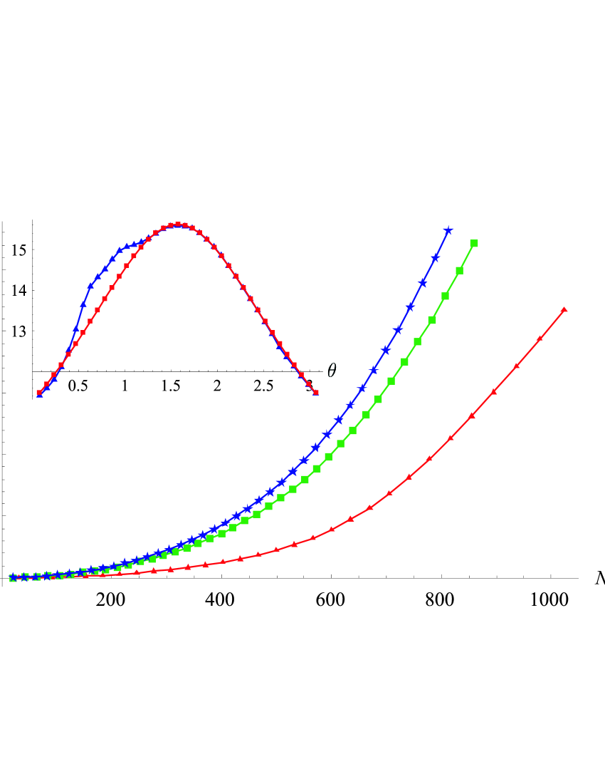
Figure 1: Relative error between ${\cal N}^{\Omega_{\theta,\phi=0}}_{yy}$ and $\tilde{N}^{\Omega_{\theta,\phi=0}}_{yy}(T)$, with respect to the number of emitted photons with $\alpha=y$, integrating all over $\theta$ for $\phi=0$. Triangles: $J/B=-0.5$, Boxes: $J/B=-0.1$, Stars: $J/B=-0.01$.; Inset: Number of $y$-polarized photons for each value of $\theta$ with $\phi=0$, with $T=0.001$ (units of $\Gamma_{0}=1$), and $J/B=-0.5$. Triangles: ${\cal N}^{\Omega_{\theta,\phi=0}}_{yy}=\Gamma_{0}N\int_{0}^{T}dt\langle J^{\theta,\phi=0}_{x}(t)J^{\theta,\phi=0}_{x}(t)\rangle$ (Emitted photons). Squares: $\tilde{N}^{\Omega_{\theta,\phi=0}}_{yy}(T)=\Gamma_{0}NT\langle J^{\theta,\phi=0}_{x}(0)J^{\theta,\phi=0}_{x}(0)\rangle$ (Emitted photons that correspond to ground state)

The information gathered by measuring in different directions, may be used to reconstruct atomic correlations in the position space. To study the conditions which are required for this task, we focus on the particular example of a $2D$ optical lattice. This case is relevant to the characterization of cluster states and experiments which simulate high–Tc superconductors. Consider also for concreteness that the incident laser propagates along the $z$ direction, and that the lattice is defined within the $x$-$y$ plane. Following (6), an homodyne detection of the quadrature $\mathcal{X}^{\bf k}_{\alpha}$ allows one to measure the operator $J_{C\beta}^{\Delta{\bf k}}$, where now we have that $\Delta{\bf k}=k_{\textmd{L}}(\sin\theta\cos\phi,\sin\theta\sin\phi,\cos\theta-1)$. Then the spin operator $J^{(n,m)}_{C\beta}=J_{\beta}^{(n,m)}+J_{\beta}^{(-n,-m)}$ in the position space, with $(n,m)$ denoting a particular site within the lattice, can be obtained as an inverse Fourier transform of $J_{C\beta}^{\Delta{\bf k}}$,

$$J^{(n,m)}_{C\beta}=C\int^{1}_{-1}d\tilde{k}_{x}\int^{1}_{-1}d\tilde{k}_{y}\cos(\tilde{k}_{x}n\pi+\tilde{k}_{y}m\pi)J_{C\beta}^{\Delta{\bf k}},$$ (9)

where we have defined $C=\sqrt{N}/2$, and the integration variables as $\tilde{\bf k}=(r_{0}/\pi)\Delta{\bf k}$. By changing the detection angles ($\theta,\phi$), it is possible to measure the quantity $J_{C\beta}^{\Delta{\bf k}}$ for values of ${\Delta{\bf k}}$ that lie within a circle of radius $R_{0}=2k_{\textmd{L}}r_{0}/\pi$. The integral (9) has to be sampled with a set of values of $J_{C\beta}^{\Delta{\bf k}}$ within the region of integration defined by the square $\tilde{k}_{x}\epsilon[-1,1]$, and $\tilde{k}_{y}\epsilon[-1,1]$. Therefore, a basic requirement to obtain $J^{(n,m)}_{C\beta}$ is to chose $r_{0}k_{L}\geq\sqrt{2}\pi$, so that the integration region is contained within the circle $R_{0}$. Note that this implies that $k_{L}/k_{latt}\geq\sqrt{2}$, where $k_{latt}$ is wavelength of the standing wave lasers. An additional homodyne detection of the quadrature $\mathcal{P}_{\alpha}^{\bf k}=i\epsilon_{\bf k}(a^{\dagger}_{{\bf k}\alpha}-a_{{\bf k}\alpha})$, allows one to obtain the quantity $J^{(n,m)}_{S\beta}=J_{\beta}^{(n,m)}-J_{\beta}^{(-n,-m)}$, which combined with (9) can be used to measure the operator $J_{\beta}^{(n,m)}$. Correlations in 3D can be obtained provided that both the direction of photon detection, and the direction of the incident laser are tuned to scan the whole momentum space. Following the same argument as before, the condition to get spatial information is $r_{0}k_{L}\geq\sqrt{3}\pi$.

Once the operators $J_{\beta}^{(n,m)}$ are obtained as the inverse Fourier transforms of field quadratures, it is straightforward to calculate their correlations. These spatial correlations are useful to characterize some interesting states, like for instance cluster states $|\phi\rangle_{cl}$. The later are defined by a set of eigenvalue equations for the operator $K^{j}=\sigma_{x}^{j}\bigotimes_{l\epsilon neigh(j)}\sigma_{z}^{l}$, such that $K^{j}|\phi\rangle_{cl}=\pm|\phi\rangle_{cl}$ RB01 ; RBB03 , where $neigh(j)$ specifies the sites of all atoms $l$ that interact with an atom $j$. With this definition at hand, a cluster state in a $2D$ lattice can be characterized by checking that the spatial correlation $\langle J^{(n_{1},m_{1})}_{z}J^{(n_{1},m_{2})}_{z}J^{(n_{3},m_{3})}_{x}J^{(n_{4},m_{4})}_{z}J^{(n_{5},m_{5})}_{z}\rangle$ is equal to $\pm 1$ when the operators $J_{z}$ are next neighbors of $J_{x}$. These spatial correlations can be obtained by making an inverse Fourier transform of the quantity $\langle J_{z}^{\Delta{\bf k}_{1}}J_{z}^{\Delta{\bf k}_{2}}J_{x}^{\Delta{\bf k}_{3}}J_{z}^{\Delta{\bf k}_{4}}J_{z}^{\Delta{\bf k}_{5}}\rangle$, that may be measured by considering a $y$ polarized laser and correlations of different homodyne detections of quadratures. Then, the inverse transform can be made following the basic relation (9), and the analogous relation that exists for $J^{(n,m)}_{S\beta}$. This scheme can be readily extended to measure many operator averages which characterize magnetic quantum phases, like for example, the valence bond strength, $\langle{\bf J}_{j}\cdot{\bf J}_{l}\rangle$, where $j$, $l$ are nearest neighbors.

One of the main limitations of the method is the fact that we need a good detection efficiency. The reason is that only a few photons are emitted at each solid angle (see Fig. (1)), because the measurement time $T$ has to be small enough to ensure that only a few atoms produce scattering and the measured state is preserved. Also, just as in TOF imaging, the reconstruction of atomic correlation functions, requires to perform each measurement $M$ times, with $M$ large so that the quantity $1/\sqrt{M}$ that characterizes the statistical error for the measurement is small. Nevertheless, one important difference with respect to TOF is that there are no limitations regarding the laser shot noise. In TOF experiments, the atomic noise has to exceed the shot noise of the prove laser. Here, the fluctuations of the prove laser can be easily distinguished and eliminated, since the laser polarization is different from the polarization of the emitted photons that we measure. Since our model is valid for measuring atoms in a Mott state, a further source of error would be the appearance of a superfluid region in the borders of the atomic cloud. This problem can be overcome by focusing the scattering laser to the center of the ensemble.

In summary, we have shown how to detect spin correlations of an atom lattice within a Mott insulator state without switching off the potential. The detection scheme is based on the fact that spin correlations in the momentum space are proportional to correlations of the photons that are emitted in an off-resonant scattering process. Using different photon detection techniques allows to measure different types of spin correlations that are useful to characterize certain many body states, like magnetic phases. A complete sampling of these correlations in the momentum space can be used to obtain spatial correlations, which are useful to characterize some other phases like cluster states.

We would like to thank Miguel Aguado for helpful discussions. Work supported by EU projects (SCALA and CONQUEST), and Cluster of Excelence Munich-Centre for Advanced Photonics (MAP). I.D.V acknowledges support from Ministerio de Educación y Ciencia.

References

(1) L.-M. Duan, E. Demler, and M.D. Lukin, Phys. Rev. Lett. 91,
090402 (2003).
(2) I. H. Deutsch, P.S. Jessen, Phys. Rev. A 57, 1972 (1998).
(3) G.K. Brennen et al. Phys. Rev. Lett. 82, 1060 (1999).
(4) D. Jacks et al., Phys. Rev. Lett. 82, 1975 (1999).
(5) O. Mandel et al. Nature 425, 937 (2003).
(6) R. Raussendorf et al. Phys. Rev. Lett. 86, 5188 (2001).
(7) R. Raussendorf et al. Phys. Rev. A 68, 022312 (2003).
(8) E. Altman et al., Phys. Rev. A 70, 013603 (2004).
(9) S. Fölling et al. Nature, 434, 481 (2005).
(10) M. Greiner et al. Phys. Rev. Lett. 94, 110401 (2005).
(11) K. Eckert et al., Phys. Rev. Lett. 98, 100404 (2007).
(12) K. Eckert et al. cond-mat/0709.0527, to be published in Nature for Physics, (2007).
(13) K. Hammerer, PHD thesis (2005).
(14) B. Julsgaard, PHD thesis (2003).
(15) The fast rotating term shall be included here to describe correctly the dipole-dipole interactions L70 .
(16) D.F. Walls, and G.J. Milburn, Quantum Optics, Springer-Verlag (1994).
(17) R. H. Lehmberg, Phys. Rev. A, 70, 883 (1970).