Coupling Lattice Boltzmann with Atomistic Dynamics for the multiscale simulation of nano-biological flows

Abstract

We describe a recent multiscale approach based on the concurrent coupling of constrained molecular dynamics for long biomolecules with a mesoscopic lattice Boltzmann treatment of solvent hydrodynamics. The multiscale approach is based on a simple scheme of exchange of space-time information between the atomistic and mesoscopic scales and is capable of describing self-consistent hydrodynamic effects on molecular motion at a computational cost which scales linearly with both solute size and solvent volume. For an application of our multiscale method, we consider the much studied problem of biopolymer translocation through nanopores: we find that the method reproduces with remarkable accuracy the statistical scaling behavior of the translocation process and provides valuable insight into the cooperative aspects of biopolymer and hydrodynamic motion.

I Introduction

Modeling biological systems in an efficient and reliable way is a delicate task, which calls for the development of innovative computational methods, often requiring sophisticated upgrades and extensions of techniques originally developed for physical and/or chemical stand-alone applications. Indeed, biological systems exhibit a degree of complexity and diversity straddling across many decades in space-time resolution, to the point that, for many years, biological systems served as a paradigm of the kind of complexity which can only be handled in qualitative or descriptive terms. Advances in computer technology, combined with constant progress and breakthroughs in simulational methods, are closing the gap between quantitative models and actual biological behavior. The main computational challenge raised by biological systems remains the wide and disparate range of spatio-temporal scales involved in their dynamical evolution, with protein folding, morphogenesis, intra- and extra-cellular communication, being just a few examples.

In response to this challenge, various strategies have been developed recently, which are in general referred to as multiscale modeling. These methods are based on composite computational schemes which rely upon multiple levels of description of a given biological system, most typically the atomistic and continuum levels. The multiple descriptions are then glued together, through suitable ’hand-shaking’ procedures, to produce the final composite multiscale algorithm. To date, the mainstream multiscale modeling is based on the coupling between atomistic and continuum models. This choice reflects the historical developments of statistical mechanics and computational physics. In essence, continuum methods reduce the information to a small number of distributed properties (fields), whose space-time evolution is computed by solving a corresponding set of partial differential equations, such as reaction-diffusion-advection equations. Atomistic models, on the other hand, rely on the well established approach of molecular dynamics, possibly including extensions capable of dealing with a quantum description. It is perhaps interesting to notice that this two-stage continuum-to-atomistic representation overlooks a third, intermediate, level of description, that is the mesoscopic level, as typically represented by Boltzmann kinetic theory and its extensions. Kinetic theory lies between the continuum and atomistic descriptions, and it is thereby natural to expect that it should provide an appropriate framework for the development of robust multiscale methodologies.

Until recently, this approach has been hindered by the fact that the central equation of kinetic theory, the Boltzmann equation, was typically perceived computationally nearly as demanding as molecular dynamics, and yet of very limited use for dense fluids (water being the typical biological medium), due to the lack of many-body correlations. Recent developments in lattice kinetic theory LBE ; LBEORIG are making this view obsolete. Over the last decade, such developments have provided solid evidence that suitably discretized forms of minimal kinetic equations, and most notably the Lattice Boltzmann equation, are giving rise to very efficient algorithms capable of handling complex flowing systems across many scales of motion. The behavior of fluid flow is described through minimal forms of the Boltzmann equation, living on a discrete lattice. The lattice dynamics is designed in such a way as to reflect the basic conservation laws of continuum mechanics, and also to host additional (mesoscopic) physics which is not easily accommodated by continuum models. Remarkably, both tasks can be achieved within the same algorithm, which proves often computationally advantageous over the continuum approach based on the Navier-Stokes equations. It is only very recently that LB advances have started to be incorporated within a new class of mesoscopic multiscale solvers MULBE . In this work, we address precisely such mesoscopic multiscale solvers, with specific focus on the biologically important problem of biopolymer translocation through nanopores. Our procedure is based on the assumption that, in order to capture the essential aspects of the translocation process, it is not necessary to resolve all underlying atomistic details. As a result, both solvent and solute degrees of freedom are treated through appropriate coarse-graining. Due to the intrinsic coarse-graining nature of our methodology, the direct mapping to experimental conditions has to proceed through the adjustment of appropriate parameters.

II Multiscale coupling methodology

We will discuss the implementation of how a mesoscopic fluid solver, the lattice Boltzmann method (LB), can be coupled concurrently to the atomistic scale employing explicit atomistic dynamics which, for simplicity, will be named molecular dynamics (MD) in a broad sense. This procedure involves different levels of the statistical description of matter (continuum and atomistic) and is able to handle different scales through the spatial and temporal coupling between the constrained molecular dynamics for the polymer evolution and the lattice Boltzmann treatment of the explicit solvent dynamics. This multiscale framework is well suited to address a class of biologically related problems.

The solvent dynamics does not require any form of statistical ensemble averaging, as it is represented through a discrete set of pre-averaged probability distribution functions (the single-particle Boltzmann distributions), which are propagated along straight particle trajectories. At variance with Brownian dynamics, the lattice Boltzmann approach handles the fluid-mediated solvent-solvent interactions through an explicit representation of local collisions between the solvent and solute molecules. By leveraging space-time locality, the corresponding algorithm scales linearly with the number of beads, as opposed to the (super)quadratic dependence of Brownian dynamics. This dual field/particle nature greatly facilitates the coupling between the mesoscopic and atomistic levels, both on conceptual and computational grounds. Full details on this scheme are reported in Ref. ourLBM . It should be noted that, LB and MD have been coupled before for the investigation of single-polymer dynamics DUN , but here this coupling is extended to long molecules of biological interest.

A word of caution is in order with the Stokes limit $Re\rightarrow 0$. In this limit, the scale separation between atomistic and hydrodynamic degrees of freedom becomes opaque, as the atomic mean free path becomes comparable with hydrodynamic scales. However, it has been shown that finite Reynolds corrections to hydrodynamics have very negligible effects on the solvent-mediated forces between suspended bodies, e.g. Oseen-level hydrodynamics is satisfactorily recovered LADDVERBERG ; CATES ; ourLBM ; PREPA .

We first turn to the atomistic part within our approach and consider a polymer consisting of $N$ monomer units (also referred to as beads). Each bead of the polymer is advanced in time according to the following set of Molecular Dynamics equations:

$$\vec{F}_{tot,i}=\vec{F}_{c,i}+\vec{F}_{drag,i}+\vec{F}_{r,i}+\vec{F}_{\kappa,i}$$ (1)

where the index $i$ runs over all beads. In this expression, $\vec{F}_{c,i}$ is a conservative force describing bead-bead interactions, represented here by a Lennard-Jones potential:

$$V_{LJ}(r)=4\varepsilon\left[\left(\frac{\sigma}{r}\right)^{12}-\left(\frac{\sigma}{r}\right)^{6}\right]$$ (2)

This potential is truncated at a distance of r=$2^{1/6}\sigma$ and augmented by an angular harmonic term to account for distortions of the angle between consecutive bonds:

$$V_{ang}(\phi)=\frac{\kappa_{\phi}\phi^{2}}{2}$$ (3)

with $\phi$ the relative angle between two consecutive bonds, and $\kappa_{\phi}$ a constant. Torsional motions are not included in the present model, but can easily be incorporated if needed. The second term in Eq.(1), $\vec{F}_{drag,i}$, represents the dissipative drag force due to polymer-fluid coupling given by

$$\vec{F}_{drag,i}=-m\gamma(\vec{v}_{i}-\vec{u}_{i})$$ (4)

with $\vec{v}_{i}$, $\vec{u}_{i}$ the bead and fluid velocity evaluated at the bead position $\vec{r}_{i}$ of bead $i$ with a mass $m$; $\gamma$ is the friction coefficient. In addition to mechanical drag, the polymer feels the effects of stochastic fluctuations of the fluid environment, which is related to the third term in Eq.(1), $\vec{F}_{r,i}$, an uncorrelated random force with zero mean acting on bead $i$. The term $\vec{F}_{\kappa,i}$ in Eq.(1) is the reaction force resulting from $N-1$ holonomic constraints for molecules modelled with rigid covalent bonds. The usage of constraints instead of flexible bond lengths makes it possible to eliminate unimportant high-frequency intra-molecular motion which might lead to numerical instabilities. In order to avoid spurious dissipation, the bead velocities are required to be strictly orthogonal to the relative displacements. The constraints on both positions and velocities are enforced over positions and momenta separately via the SHAKE and RATTLE algorithms SHAKE ; RATTLE .

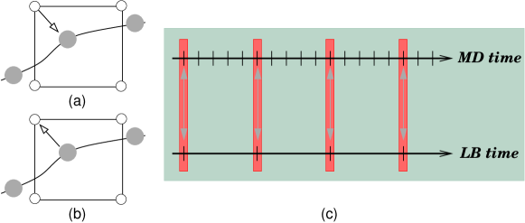
Figure 1: Transfer of spatial information (a) from grid to particle, and (b) from particle to grid. Grey spheres denote beads, while in white are the lattice sites. In (c) the information exchange (LB-MD couling) is sketched through the vertical highlighted regions between the two different scales of our multiscale approach. The MD marches in time on a finer time-scale (by a factor of 5 in the sketch and our simulations) than the LB solver.

The LB equation is a minimal form of the Boltzmann kinetic equation in which all details of molecular motion are removed except those that are strictly needed to recover hydrodynamic behavior at the macroscopic scale (mass-momentum and energy conservation). The result is an elegant equation for the discrete distribution function $f_{p}(\vec{x},t)$ describing the probability to find a LB particle at lattice site $\vec{x}$ at time $t$ with a discrete speed $\vec{c}_{p}$. Specifically, in this work we are dealing with nanoscale flows and will consider the fluctuating Lattice Boltzmann equation which takes the following form adhikari :

$$f_{p}(\vec{x}+\vec{c}_{p}\Delta t,t+\Delta t)=f_{p}(\vec{x},t)-\omega\Delta t(f_{p}-f_{p}^{eq})(\vec{x},t)+F_{p}\Delta t+S_{p}\Delta t$$ (5)

The particles can only move along the links of a regular lattice defined by the discrete speeds, so that the synchronous displacements $\Delta\vec{x}_{p}=\vec{c}_{p}\Delta t$ never take the fluid particles away from the lattice. For the present study, the standard three-dimensional 19-speed lattice is used (see Fig.1 in Ref. MULBE ). The right hand side of Eq. 5 represents the effect of intermolecular solvent-solvent collisions, through a relaxation toward local equilibrium, $f_{p}^{eq}$, typically a second order (low-Mach) expansion in the fluid velocity of a local Maxwellian with speed $\vec{u}$:

$$f_{p}^{eq}=w_{p}\rho\{1+\frac{\vec{u}\cdot\vec{c}_{p}}{c_{s}^{2}}+\frac{1}{2c_{s}^{4}}[\vec{u}\vec{u}:(\vec{c}_{p}\vec{c}_{p}-c_{s}^{2}{\rm\vbox{\halign{#\cr$\leftrightarrow$\crcr \kern-1.0pt\nointerlineskip\cr$\hfil\displaystyle{I}\hfil$\crcr}}})]\}$$ (6)

where $c_{s}$ is the sound speed of the solvent, $w_{p}$ is a set of weights normalized to unity, $\leftrightarrow$ $\hfil\displaystyle{I}\hfil$ is the unit tensor in configuration space, and $\rho$ is the local density. The relaxation frequency $\omega$ controls the fluid kinematic viscosity $\nu$, through the relation $\nu=c_{s}^{2}(1/\omega-\Delta t/2)$ MULBE and $\Delta t$ the LB time-step. Knowledge of the discrete distributions $f_{p}$ allows the calculation of the local density $\rho$, flow speed $\rho\vec{u}$ and momentum-flux tensor $\leftrightarrow$ $\hfil\displaystyle{P}\hfil$ , by a direct summation upon all discrete distributions:

$$\rho(\vec{x},t) = \sum_{p}f_{p}(\vec{x},t)$$ (7)

$$\rho\vec{u}(\vec{x},t) = \sum_{p}f_{p}(\vec{x},t)\vec{c}_{p}$$ (8)

$$\vbox{\halign{#\cr$\leftrightarrow$\crcr \kern-1.0pt\nointerlineskip\cr$\hfil\displaystyle{P}\hfil$\crcr}}(\vec{x},t) = \sum_{p}f_{p}(\vec{x},t)\vec{c}_{p}\vec{c}_{p}$$ (11)

The diagonal component of the momentum-flux tensor gives the fluid pressure, while the off-diagonal terms give the shear-stress. Both quantities are available locally and at any point in the simulation. Thermal fluctuations are included through the source term $F_{p}$ in Eq. (5), which is consistent with the fluctuation-dissipation theorem at all scales. In the same equation, the polymer-fluid back reaction is described through the source term $S_{p}$, which represents the momentum input per unit time due to the reaction of the polymer on the fluid populations. This back reaction is given by the following expression:

$$S_{p}(\vec{x},t)=\frac{w_{p}}{c_{s}^{2}}\sum_{i\in D(x)}[\vec{F}_{drag,i}+\vec{F}_{r,i}]\cdot\vec{c}_{p}$$ (12)

where $D(x)$ denotes the mesh cell to which the i^th bead belongs. All quantities in this equations have to reside on the lattice nodes, thereby the frictional and random forces need to be extrapolated from the particle to the grid location.

In the LB solver, free-streaming proceeds along straight trajectories which secures exact conservation of mass and momentum of the numerical scheme, but also greatly facilitates the imposition of geometrically complex boundary conditions. There is no need to solve the computationally expensive Poisson equations, since the pressure field is locally available. All interactions are local, rendering the LB scheme ideal for parallel computing. More advanced Lattice Boltzmann models karlin also have been developed and could equally well be suited for coupling to atomic scale dynamics.

The Molecular Dynamics solver is marched in time with a stochastic integrator (due to extra non-conservative and random terms) melchJCP , proceeding at a fraction $1/M$ of the LB time-step $\Delta t$: $\Delta t_{MD}=\Delta t/M$. The time-step ratio $M>1$ controls the scale separation between the solvent and solute timescales and should be chosen as small as possible, consistent with the requirement of providing a realistic description of the polymer dynamics. The MD cycle is repeated $M$ times, with the hydrodynamic field frozen at each LB time-stamp $t_{n}=n\Delta t$, at which the transfer of spatial information from grid to particle locations (and conversely) is performed. For this transfer, a simple nearest grid point interpolation scheme is used (see Fig.1(a), (b)), on account of its simplicity. At a time step $t_{n}=n\Delta t$, the pseudo-algorithm describing single LB time-step, will be:

1. Interpolation of the velocity: $\vec{u}(\vec{x})\rightarrow\vec{u}_{i}$

2. For $k=1,M$: Advance the molecular state from $t$ to $t+\Delta t_{MD}$

3. Extrapolation of the forces: $\vec{F_{i}}\rightarrow\vec{F}(\vec{x})$

4. Advance the Boltzmann populations from $t$ to $t+\Delta t$

A sketch of this scheme is presented in Fig. 1. In terms of computational efficiency, $\Delta t_{MD}$ is largely independent of the number of beads $N$ because (i) the LB-MD coupling is local, (ii) the forces are short ranged and (iii) the SHAKE/RATTLE algorithms are empirically known to scale linearly with the number of constraints. Up to this point we described a scheme that is general and applicable to any situation where a long polymer is moving in a solvent. This motion is of great interest for a fundamental understanding of polymer dynamics in the presence of the solvent and crucial in relevant biophysical processes.

III Biopolymer translocation through nanopores

We next turn to an application of the multiscale scheme described in the previous section. We were motivated by recent experimental studies which have focused on the translocation of biopolymers such as RNA or DNA through nanometer sized pores. These explore in vitro the translocation process through micro-fabricated channels under the effects of an external electric field, or through protein channels across cellular membranes EXPRM . In particular, recent experimental work has focussed on the possibility of fast DNA-sequencing through electronic means, that is, by reading the DNA sequence while it is moving through a nanopore under the effect of a localized electric field EXPRM . This type of biophysical processes are important in phenomena like viral infection by phages, inter-bacterial DNA transduction or gene therapy TRANSL . Some universal features of DNA translocation have also been analyzed theoretically, by means of suitably simplified statistical schemes statisTrans , and non-hydrodynamic coarse-grained or microscopic models DynamPRL ; coarse . However, these complex phenomena involve the competition between many-body interactions at the atomic or molecular scale, fluid-atom hydrodynamic coupling, as well as the interaction of the biopolymer with wall molecules in the region of the pore. Resolving these interactions is essential in understanding the physics underlying the translocation process. To this end, we model the dynamics of biopolymer translocation through narrow pores, using the multiscale scheme described above.

Our numerical simulations are performed in a three-dimensional box of size $N_{x}\times N_{y}\times N_{z}$ in units of the lattice spacing $\Delta x$. The box contains both the solvent and the polymer. We take $N_{x}=2N_{y}$, $N_{y}=N_{z}$; a separating wall is located in the mid-section of the $x$ direction, at $x=N_{x}/2$. For polymers with less than $500$ beads we use $N_{x}=80$ while for larger polymers $N_{x}=100$. At $t=0$ the polymer resides entirely in the right chamber at $x>N_{x}/2$. At the center of the separating wall, a square hole of side $d=3\Delta x$ is opened up, through which the polymer can translocate from one chamber to the other. A 3-D representation of a typical translocation event is shown in Fig.2. The magnitude of the fluid speed is also mapped on different planes and as a 3-D contour surface surrounding the polymer beads.

Figure 2: A typical translocation event: The 3-D box including the fluid and the polymer, as well as the wall (not shown) that separates the box into two chambers. A polymer (red beads) representing double-stranded DNA is shown at an instant where about $60$% of the beads have translocated. The fluid is also shown as a 3-D representation of the velocity magnitude at the vicinity of the beads and on 2-D planes (red denotes high value). Translocation is induced by means of a pulling force $F_{drive}$ with a direction from right to left.

We elaborate next on the main parameters involved in the simulation (additional details are provided in Ref. ourLBM ). All parameters are measured in units of the lattice Boltzmann time-step $\Delta t$ and spacing $\Delta x$, which are set equal to 1. The parameters for the Lennard-Jones potential are $\sigma=1.8$, and $\epsilon=2\times 10^{-3}$ and the bond length among the beads is set to $b=1.2$. The solvent density and kinematic viscosity are $1$ and $0.1$, respectively, and the inverse temperature is $\beta=10^{4}$. It must be noted that the friction coefficient taken as $\gamma=0.1$ is a parameter governing both the structural relation of the polymer towards equilibrium and the strength of the coupling with the surrounding fluid. The MD time-step is a $1/M$ fraction of the LB time-step, as mentioned previously, and we set $M=5$.

Translocation is induced by a constant electric force, $\vec{F}_{drive,i}$, which acts along the $x$ direction and is confined in a rectangular channel of size $3\Delta x\times\Delta x\times\Delta x$ along the streamwise ($x$ direction) and cross-flow ($y,z$ directions). This force is included as an additional term in Eq.(1), and is the driving force representing the effect of the external field in the experiments. We use $F_{drive,i}=0.02$. This choice of parameter values implies that we are describing the fast translocation regime, in which the translocation time is much smaller than the Zimm time, which is the typical relaxation time of the polymer towards its native (minimum energy, maximum entropy) configuration. Under these conditions, the many-body aspects of the polymer dynamics cannot be ignored because the beads along the chain do not move independently.

Here, we model DNA as a polymeric chain of a number of segments (the beads) and trace its dynamic evolution interacting with a fluid solvent as it passes through a narrow hole that is comparable with the bead size. Each bead maps to a number of base-pairs (bp), ranging from about 8 (similar to the hydrated diameter of B-DNA in physiological conditions) to $\sim 10^{3}$ beadParam1 ; beadParam2 . In order to estimate this number for our simulations and interpret our results in terms of physical units we examine the persistence length ($l_{p}$) of the semiflexible polymers used in our simulations. We use the formula for the fixed-bond-angle model of a worm-like chain lpWCL :

$$l_{p}=\frac{b}{1-\cos\langle\theta\rangle}$$ (13)

where $\langle\theta\rangle$ is complementary to the average bond angle between adjacent bonds. In lattice units ($\Delta x$) an average persistence length for the polymers considered was found to be approximately $12$. For $\lambda$-phage DNA, $l_{p}\sim 50$ nm lpDNA , which is set equal to $l_{p}$ for our polymers. Thereby, the lattice spacing is $\Delta x\sim 4$ nm, which is also the size of one bead. Given that the base-pair spacing is $\sim 0.34$ nm, one bead maps to approximately $12$ base pairs. With this mapping, the pore size is about $\sim 12$ nm, close to the experimental pores which are of the order of $10$ nm. The polymers presented here with $N=20-500$ beads correspond to DNA lengths in the range $0.2-6\times 10^{3}$ bp. The DNA lengths used in the experiments are larger (up to $\sim 10^{5}$ bp); with appropriate computational resources, our multiscale scheme could handle these lengths.

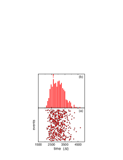
Figure 3: (a) The variety of different translocation events and the corresponding translocation times; (b) from the events in (a) the duration histogram is extracted for a molecule with 100 beads, which represents double-stranded DNA with $1.2$ kbp. Time is given in units of the LB time-step $\Delta t$.

Having established the quantitative mapping of DNA base-pairs to the simulated beads, we seek a comparison of the statistical features of the simulated translocation process to experimental studies. The ensemble of our simulations is generated by different realizations of the initial polymer configuration to account for the statistical nature of the process. We performed extensive simulations of a large number of translocation events over $100-1000$ initial polymer configurations for each polymer length. The various events for a given length are depicted in Fig. 3(a). The projected duration histograms are shown in Fig. 3(b) in LB units. Similar distributions were obtained for all the polymer lengths considered here, by accumulating all events for each length. By choosing lengths that match experimental data we compare the corresponding experimental duration histograms (see Fig. 1c of Ref. NANO ) to the theoretical ones. This comparison sets the LB time-step to $\Delta t\sim 8$ nsec. In Fig. 4 we show the time distributions for representative DNA lengths simulated here. In this figure, physical units are used according to the mapping described above for direct comparison to similar experimental data NANO . The MD time-step for $M=5$ will then be $\Delta t_{MD}\sim 1.6$ nsec indicating that the MD timescale related to the coarse-grained model that handles the DNA molecules is significantly stretched over the physical process. Exact match to all the experimental parameters is of course not feasible with coarse-grained simulations. Nevertheless, essential features of DNA translocation are reasonably well reproduced, allowing the use of the current approach to model similar biophysical processes that involve biopolymers in solution. This can become more efficient by exploiting the freedom of further fine-tuning the parameters used in the multiscale model.

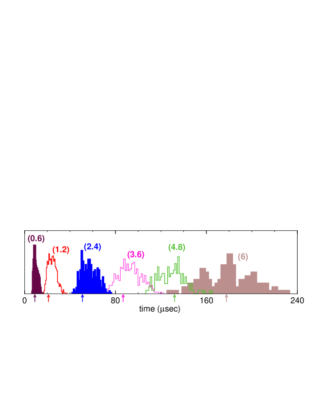
Figure 4: Histograms of calculated translocation times for a large number of events and various DNA lengths shown in parentheses in kbp ($10^{3}$ bp). The arrows point to the most probable time for each polymer size.

The variety of all the different initial polymer realizations produce a scaling law dependence of the translocation times on length coarse ; NANO . The duration histograms are not simple gaussians, but are rather skewed towards longer times. Accordingly, we use the most probable time (peak of the distribution shown by the arrow in Fig. 3(b)) as the representative translocation time for every distribution; this is also the definition of the translocation time in experiments, to which we compare our results. Calculating the most probable times for each length leads to the nonlinear relation between the translocation time $\tau$ and the number of beads $N$: $\tau(N)\propto N^{\alpha}$, with an exponent $\alpha\sim 1.28\pm 0.01$. The scaling law is reported in Fig. 5 and is in very good agreement with a recent experimental study of double-stranded DNA translocation, that reported $\alpha\simeq 1.27\pm 0.03$ NANO . In the absence of a solvent the exponent rises to $1.36\pm 0.03$. Such a difference indicates a significant acceleration of the process due to hydrodynamic interactions.

III.1 Dynamics of the translocation process

We next turn to the dynamics of the biopolymer as it passes through the pore. The simulations confirm that the polymer moves through the pore in the form of two almost compact blobs on either side of the wall. One of the blobs (the untranslocated part, denoted by $U$) is contracting and the other (the translocated part, denoted by $T$) is expanding. This behavior is visible in Fig. 2 for a random event and holds throughout the process, apart from the end points (initiation and completion of the translocation). A radius of gyration $R_{I}(t)$ (with $I=U,T$) can be assigned to each of these blobs, following a static scaling law with the number of beads $N_{I}$: $R_{I}(t)\sim N_{I}^{\mu}(t)$ with $\mu\simeq 0.6$ being the Flory exponent for a three-dimensional self-avoiding random walk. Based on the conservation of polymer length, $N_{U}+N_{T}=N$, an effective translocation radius can be defined as

$$R_{E}(t)=[R_{T}^{1/\mu}(t)+R_{U}^{1/\mu}(t)]^{\mu}$$ (14)

which should be constant when the static scaling applies. We deduce from our simulations that $R_{E}(t)$ is approximately constant for all times throughout the process except near the end points, at which the polymer can no longer be represented as two uncorrelated compact blobs and the static scaling no longer holds.

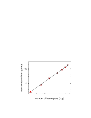
Figure 5: Scaling law of the translocation time with the DNA length.

In Fig. 6(a), we represent the time evolution of all radii as averages over hundreds of events for a specific polymer length. The time shown is scaled so that $t=1$ denotes the total translocation time for an event. By definition, $R_{U}(t)$ vanishes at $t=1$, while $R_{T}$ increases monotonically from $t=0$ up to $t=1$, although it never reaches the value $R_{U}(t=0)$ (we elaborate on this below).

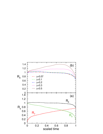
Figure 6: (a) Radii of gyration (translocated, untranslocated and effective) for a polymer representing $4.8$ kbp as a function of time. (b) Effective radii of gyration with time for different values of the coupling $\gamma$ ($N=200\sim 2.4~{}kbp$). Time and $R_{E}$ are scaled with respect to the total translocation time and $R_{U}(t=0)$ for each case.

It is essential to check the validity of the static scaling with respect to the strength of the hydrodynamic field. To this end, the effective radii of gyration are further explored in relation to the parameter $\gamma$. We fixed the length to $N=200$ beads and generated about 100 different initial configurations for each value of $\gamma$. We present the variation of $R_{E}$ with this coefficient in Fig. 6(b): It is clearly visible in this figure that $R_{E}$ is almost constant for small $\gamma$ but as $\gamma$ increases, the radii are no more constant not only at the end points, but also throughout the translocation. Large values of the parameter $\gamma$ are interpreted as a strong molecule-fluid coupling. The influence of the fluid on the beads, experienced by the back reaction, is large and suppresses the polymer fluctuations in such a way that the translocating biopolymer can no longer be represented as a pair of compact blobs, and the static scaling no longer holds.

Inspection of all the biopolymers at the end of the event reveals that they become more compact after their passage through the pore. This is quantitatively checked through the values of the radii of gyration: the radius of gyration is considerably smaller at the end than it was initially: $R_{T}(t=1)<R_{U}(t=0)$. The fact that as the polymer passes through the pore it becomes more compact than it was at the initial stage of the event may be related to incomplete relaxation, but this remains to be investigated. In Fig. 6(b), all effective radii of gyration at the final stage of the translocation decrease to a value smaller than the initial $R_{U}(t=0)$. The ratio $R_{T}(t=1)/R_{U}(t=0)$ is always smaller than 1 and ranges from $0.72$ for $\gamma$=0.1 to $0.90$ for $\gamma$=0.5.

Throughout its motion the polymer continuously interacts with the fluid environment. The forces that essentially control the process are the electric drive $\vec{F}_{drive,i}$ and the hydrodynamic drag $\vec{F}_{drag,i}$ which act on each bead. However, at the end points (initiation and completion of the passage through the pore) entropic forces become important blob . The fluctuations experienced by the polymer due to the presence of the fluid are correlated to these entropic forces which, at least close to equilibrium, can be expressed as the gradient of the free energy with respect to the fraction of translocated beads. At the final stage of a translocation event, the radius of the untranslocated part undergoes a visible deceleration (see Fig. 6(a)), the majority of the beads having already translocated. It is, thus, entropically more favorable to complete the passage through the hole rather than reverting it, that is, the entropic forces cooperate with the electric field and the translocation is accelerated.

The entropic forces can also lead to rare events, such as retraction, which occur in our simulations at a rate less than 2% and depend on length, initial polymer configuration and parameter set. A retraction event is related to a polymer that anti-translocates after having partially passed through the pore. We have visually inspected the retraction events and associate them with the translocated part entering a low-entropy configuration (hairpin-like) subject to a strong entropic pull-back force from the untranslocated part: The translocated part of the polymer assumes an elongated conformation, which leads to an increase of the entropic force from the coiled, untranslocated part of the chain. As a result, the translocation is delayed and eventually the polymer is retracted.

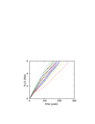
Figure 7: Time evolution of the number of translocated beads $N_{T}(t)$ for DNA with $6$ kbp. Curves correspond to translocation events for a variety of different initial configurations.

The fact that the entropic forces are related to the number of translocated monomers $N_{T}(t)$ led us to investigate in more detail the time evolution of this quantity. The number of translocated monomers is plotted in Fig.7 for various initial configurations of the polymer. Each curve corresponds to a different completed translocation event. The translocation for a given polymer proceeds along a curve closely related to its initial configuration and its interactions with the fluid; each polymer follows a distinct trajectory as indicated by the variety of curves. It is not possible to predict the ensuing behavior from the initial polymer configuration in a simple and unique manner.

III.2 Energetics of the translocation process

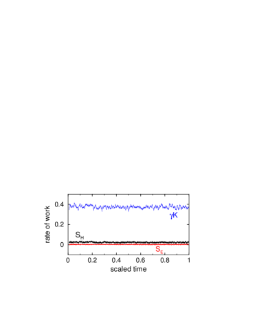
Figure 8: Rates of work ($S_{H}$, $S_{E}$) and kinetic energy ($\gamma K$) as functions of time for one translocation event of a polymer consisting of $N=300$ beads ($3.6$ kbp). Time is scaled with respect to the total time of this event.

As a final step, we study the work performed on the biopolymer throughout its translocation. On general grounds, hydrodynamic interactions are expected to minimize frictional effects and form a cooperative background that assists the passage of the polymer through the pore. We investigate the cooperativity of the hydrodynamic field through the synergy factor $S_{H}(t)$ defined as the work made by the fluid on the polymer per unit time:

$$S_{H}(t)=\frac{dW_{H}}{dt}=\gamma\Big{\langle}\sum_{i}^{N}\vec{v}_{i}(t)\cdot\vec{u}_{i}(t)\Big{\rangle}$$ (15)

where $W_{H}$ is the work of the fluid on the polymer. Through this definition, positive values of this hydrodynamic work rate indicate a cooperative effect of the solvent, while negative values indicate a competitive effect by the solvent. The work done per timestep by the electric field ($S_{E}(t)$) on the polymer can also be easily obtained through the expression:

$$S_{E}(t)=\frac{dW_{E}}{dt}=\Big{\langle}\sum_{i}^{N}\vec{F}_{drive,i}\cdot\vec{v}_{i}(t)\Big{\rangle}$$ (16)

where $W_{E}$ is the work of the electric drive on the polymer. The brackets in Eq.(15) and (16) denote averages over different realizations of the polymer for the same length. The results for the averages over all realizations are qualitatively similar to the work rates for an individual event of the same length. For all lengths studied here, we found that the total work per timestep of the hydrodynamic field ($S_{H}(t)$) on the whole chain is essentially constant, as shown in Fig. 8 for an individual event. For the same event, $S_{E}(t)$ is also constant with time. In the same figure the kinetic energy $K$ of the polymer (plotted as $\gamma K$) for the same event is shown for comparison. The kinetic energy is also constant with time, as expected since the temperature in the simulations is held constant, but its fluctuations differ from those of $S_{E}$ and $S_{H}$. The larger value of $K$ with respect to both $S_{H},~{}S_{E}$ can be justified by the fact that the bead velocities are larger compared to the fluid velocity. The hydrodynamic work per time is also larger than the corresponding electric field work, because the latter only acts in the small region around the pore. The average of all these quantities over all events for the same polymer length are also constant, and show smaller fluctuations with time than those of any individual event.

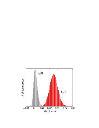
Figure 9: Distribution of the translocation work per unit time averaged over all events for a molecule with $3.6$ kbp. The contributions from both the hydrodynamic and electric field are shown: $S_{H}(t)$ and $S_{E}(t)$, respectively.

In addition to the variation of the work rates with time it is useful to analyze their distributions during translocation events. We show these in Fig. 9, where it is evident that the distribution of $S_{H}(t)$ lies entirely in the positive range, indicating that hydrodynamics turns the solvent into a cooperative environment (it enhances the speed of the translocation process). In the same figure, the distribution for $S_{E}(t)$ over all events for the same length is also shown; this distribution is mostly positive but has a small negative tail which indicates that beads can be found moving against the electric field.

III.3 Performance data

We turn next to some technical aspects of or multiscale simulations. The total cost of the computation scales roughly like

$$t\sim(t_{LB}V+t_{MD}MN)N_{LB}$$

where $t_{LB}$ is the CPU time required to update a single LB site per timestep and $t_{MD}$ is the CPU time to update a single bead per timestep (including the overhead of LB-MD coupling); $V$ is the volume of the computational domain in lattice units and $N$ is the number of polymer beads, with $M$ the LB-MD time-step ratio; $N_{LB}$ is the number of LB timesteps. Due to the fact that the LB-MD coupling is local, the forces are short ranged and the SHAKE/RATTLE algorithms are empirically known to scale linearly with the number of constraints, so that $t_{MD}$ is largely independent of $N$. The LB part is known to scale linearly with the volume occupied by the solvent. Indeed, at constant volume, the CPU cost of the simulations scales linearly with the number of beads: The execution times for $50$, $100$ and $400$ beads are $0.433$, $0.489$, and $0.882$ sec/step, respectively on a 2GHz AMD Opteron processor. By excluding hydrodynamics, these numbers become $0.039$, $0.075$, and $0.318$ sec/step. For the case where polymer concentration is kept constant, the volume needed to accommodate a polymer of $N$ beads should scale approximately as $N^{1.8}$. A typical translocation event with $500$ beads, evolves over $30,000$ LB steps or $150,000$ MD steps. Assuming $250$ flops/site/LB-step and $2500$ flops/bead/MD-step, the previous equation leads to a computational cost of $\sim 6$ hrs. This is comparable with the time observed directly from the simulations ($\sim 7$ hrs).

IV Conclusions

We have presented a new multiscale methodology based on the direct coupling between atomistic motion and mesoscopic hydrodynamics of the surrounding solvent. Due to the particle-like nature of the mesoscopic lattice Boltzmann solver, this coupling proceeds via simple interpolation/extrapolation in space and subcycling over time. Correlations between the atomistic and hydrodynamic scales are also explicitly included through direct and local interactions between the solvent meso-molecules and the polymer molecules. As a result, hydrodynamic interactions between the polymer and the surrounding fluid are explicitly taken into account, with no need of resorting to non-local representations, such as the long-range Oseen tensor used in Brownian dynamics. This allows a state-of-the-art modeling of biophysical phenomena, where hydrodynamic correlations play a significant role.

We have successfully applied our multiscale methodology to the problem of biopolymer translocation through nanoscale pores. Besides statistical properties, such as scaling exponents, the present methodology affords direct insights into the details of the dynamics as well as the energetics of the translocation process, thereby offering a very valuable complement to experimental investigations of these complex and fascinating biological phenomena. It also shows a significant potential to deal with problems that combine complex fluid motion and molecule dynamics. The efficiency of this scheme is also based on its relatively low computational demand. The molecular part is largely independent on the length of the molecule; the cost of the mesoscopic (LB) part is known to scale linearly with the volume occupied by the solvent. The linear scaling of the CPU time with the molecular size (at constant volume) is the key feature of the LB-MD approach, which permits the exploration of long biomolecules ($N>1000$) with a relatively modest computational cost. Nevertheless, resort to parallel computing is mandatory, and we expect the favorable properties of LB towards parallel implementations to greatly facilitate this task. This will also open the way to the simulation of systems at least an order of magnitude larger than those considered so far, making it possible to assign chemical specificity to the biopolymer constituents, rather than the generic nature of the beads that constitute the model polymers in the present study. Work along these lines is in progress.

- (1) D. A. Wolf-Gladrow, ”Lattice gas cellular automata and lattice Boltzmann models”, Springer Verlag, New York 2000; S. Succi, ”Lattice Boltzmann Equation for Fluid Dynamics and Beyond”, Oxford University Press, Oxford 2001; R. Benzi, S. Succi, and M. Vergassola, ”The lattice Boltzmann-equation - Theory and applications”, Phys. Rep., vol. 222, Dec. 1992, pp. 145–197.
- (2) G. McNamara, G. Zanetti, ”Use of the Boltzmann-equation to simulate lattice-gas automata”, Phys. Rev. Lett., vol. 61, no. 20, Nov. 1988, pp. 2332–2335; F. Higuera, S. Succi, and R. Benzi, ”Lattice gas-dynamics with enhanced collisions”, Europhys. Lett., vol. 9, no. 4, Jun. 1989, pp. 345–349; F. Higuera, J. Jimenez, ”Boltzmann approach to lattice gas simulations”, Europhys. Lett., vol. 9, no. 7, Aug. 1989, pp. 663–668; H. Chen, S. Chen, W. Matthaeus, ”Recovery of the Navier-Stokes equations using a lattice-gas Boltzmann method”, Phys Rev A, vol. 45, no. 8, Apr. 1992, pp. R5339–R5342; Y. H. Qian, D. d’Humieres, and P. Lallemand, ”Lattice BGK models for Navier-Stokes equation”, Europhys. Lett., vol. 17, no. 6, Feb. 1992, pp. 479–484; I.V. Karlin, A. Ferrante, H.C. Öttinger, ”Perfect entropy functions of the Lattice Boltzmann method, Europhys. Lett., vol. 47, no. 2, Jul. 1999, pp. 182–188.
- (3) S. Succi, O. Filippova, G. Smith and E. Kaxiras, ”Applying the lattice Boltzmann equation to multiscale fluid problems”, Comput. Sci. Eng., vol. 3, no. 6, Nov-Dec 2001, pp. 26–37.
- (4) M. G. Fyta, M. Melchionna, E. Kaxiras, and S. Succi, ”Multiscale coupling of molecular dynamics and hydrodynamics: application to DNA translocation through a nanopore”, Multiscale Model. Sim., vol. 5, no. 4, Dec. 2006, pp. 1156–1173.
- (5) P. Ahlrichs and B. Duenweg, ”Lattice-Boltzmann simulation of polymer-solvent systems, Int. J. Mod. Phys. C, vol. 9, no. 8, Dec. 1998, pp. 1429–1438; ”Simulation of a single polymer chain in solution by combining lattice Boltzmann and molecular dynamics”, J. Chem. Phys., vol. 111, no. 17, Nov. 1999, pp. 8225–8239; A. Chatterji, J. Horbach, ”Combining molecular dynamics with Lattice Boltzmann: A hybrid method for the simulation of (charged) colloidal systems, J. Chem. Phys., vol. 122, no. 18, May 2005, Art. No. 184903.
- (6) A.J.C. Ladd and R. Verberg. ”Lattice-Boltzmann simulations of particle-fluid suspensions”. J. Stat. Phys., vol. 104, (2001) pp. 1191-1251.
- (7) M. E. Cates, K. Stratford, R. Adhikari, P. Stansell, J. C. Desplat, E. Pagonabarraga and A. J. Wagner, “Simulating colloid hydrodynamics with Lattice Boltzmann methods”, J.Phys.Condensed Matter, vol. 16, Aug. 2004, pp. S3903–S3910.
- (8) S. Melchionna, J. Russo, S. Succi, ”Lattice Boltzmann simulation of hydrodynamic few-body correlations”, in preparation.
- (9) J. P. Ryckaert, G. Ciccotti, and H. J. C. Berendsen, ”Numerical-integration of cartesian equations of motion of a system with constraints - Molecular-Dynamics of n-alkanes”, J. Comp. Phys., vol. 23, no. 3, 1977, pp.327–341.
- (10) H. C. Andersen, ”Rattle - A velocity version of the SHAKE algorithm for Molecular-Dynamics calsulations”, J. Comput. Phys., vol. 52, no. 1, (1983), pp. 24–34.
- (11) R. Adhikari, K. Stratford, M. E.Cates and A.J. Wagner, “Fluctuating Lattice Boltzmann”, Europhys.Lett., vol. 71, no. 3, Aug. 2005, pp. 473–477.
- (12) S. Ansumali, I.V. Karlin and H.C. Höttinger, ”Minimal entropic kinetic models for hydrodynamics”, Europhys. Lett., vol. 63, no. 6, Sep. 2003, pp. 798-804; S. Ansumali and I.V. Karlin, ”Consistent Lattice Boltzmann method”, Phys. Rev. Lett., vol. 95, no. 16, Dec. 2005, Art. No. 260605.
- (13) S. Melchionna, ”Design of quasi-symplectic propagators for Langevin dynamics”, J. Chem. Phys., in press.
- (14) J. J. Kasianowicz, E. Brandin, D. Branton, D., and D. W. L Deamer, ”Characterization of individual polynucleotide molecules using a membrane channel”, Proc. Nat. Acad. Sci. USA, vol. 93, no. 24, Nov. 1996, pp. 13770–13773; A. Meller, L. Nivon, E. Brandin, J. Golovchenko, and D. Branton, ”Rapid nanopore discrimination between single polynucleotide molecules”, vol. 97, no. 3, Feb. 2000, pp. 1079–1084; J. Li, M. Gershow, D. Stein, E. Brandin, and J. A. Golovshenko, ”DNA molecules and configurations in a solid-state nanopore microscope”, Nat. Mater., vol. 2, no. 9, Sep. 2003, pp. 611–615.
- (15) H. Lodish, D. Baltimore, A. Berk, S. Zipursky, P. Matsudaira, and J. Darnell, ”Molecular Cell Biology”, W.H. Freeman and Company, New York, 1996.
- (16) W. Sung and P. J. Park, ”Polymer translocation through a pore in a membrane”, Phys. Rev. Lett., vol. 77, no. 7, Feb. 1996, pp. 783–786.
- (17) S. Matysiak, A. Montesi, M. Pasquali, A. B. Kolomeisky, and C. Clementi, ”Dynamics of polymer translocation through nanopores: Theory meets experiment”, Phys. Rev. Lett., vol. 96, no. 11, Mar. 2006, Art. No. 118103.
- (18) D. K. Lubensky and D. R. Nelson, ”Driven polymer translocation through a narrow pore” Biophys. J., vol. 77, no. 4, Oct. 1999, pp. 1824–1838 ; Y. Kantor and M. Kardar, ”Anomalous dynamics of forced translocation”, Phys. Rev. E, vol. 69, no. 2, Feb. 2004, Art. No. 021806.
- (19) A. J. Spakowitz and Z-G. Wang, ”DNA packaging in bacteriophage: Is twist important?”, Biophys. J., vol. 88, no. 6, Jun. 2005, pp. 3912–3923; C. Forrey and M. Muthukumar, ”Langevin dynamics simulations of genome packing in bacteriophage”, Biophys. J., vol. 91, no. 1, pp. 25–41 (2006) and references therein.
- (20) T. T. Perkins, D. E. Smith, S. Chu, ”Single polymer dynamics in an elongational flow”, Science, vol. 276, no. 5321, Jun. 1997, pp. 2016–2021; J. S. Hur, E. S. G. Shaqfeh, and R. G. Larson, ”Brownian dynamics simulations of single DNA molecules in shear flow”, J. Rheol., vol. 44, no. 4, Jul.-Aug. 2000, pp. 713–742; R. M. Jendrejack, J. J. de Pablo, and M. D. Graham, ”Stochastic simulations of DNA in flow: Dynamics and the effects of hydrodynamic interactions”, J. Chem. Phys., vol. 116, no. 17, May 2002, pp. 7752–7759.
- (21) Yamakawa, H. ”Modern Theory of Polymer Solutions”, Harper & Row, New York, 1971.
- (22) P. J. Hagerman, ”Flexibility of DNA”, Annu. Rev. Biophys. Biophys. Chem., vol. 17, 1988, pp. 265–286; S. Smith, L. Finzi, and C. Bustamante, ”Direct mechanical measurement of the elasticity of single DNA molecules by using magnetic beads”, Science, vol. 258, no. 5085, Nov. 1992, pp. 1122–1126.
- (23) A. J. Storm, C. Storm, J. H. Chen, H. Zandbergen, J. F. Joanny, and C. Dekker, ”Fast DNA translocation through a solid-state nanopore”, Nanolett., vol. 5, no. 7, Jul. 2005, pp. 1193–1197.
- (24) M. Fyta, S. Melchionna, S. Succi, and E. Kaxiras, “Multiscale simulations of a translocating biopolymer through a nanopore: Evidence for hydrodynamic correlations on molecular motion”, under review.