Quantum Monte Carlo Study of a Dynamic Hubbard Model

Abstract

The ‘dynamic’ Hubbard Hamiltonian describes interacting fermions on a lattice whose on-site repulsion is modulated by a coupling to a fluctuating bosonic field. We investigate one such model, introduced by Hirsch, using the determinant Quantum Monte Carlo method. Our key result is that the extended $s$-wave pairing vertex, repulsive in the usual static Hubbard model, becomes attractive as the coupling to the fluctuating Bose field increases. The sign problem prevents us from exploring a low enough temperature to see if a superconducting transition occurs. We also observe a stabilization of antiferromagnetic correlations and the Mott gap near half-filling, and a near linear behavior of the energy as a function of particle density which indicates a tendency toward phase separation.

I Introduction

The fermion Hubbard Hamiltonian fazekas99 , originally proposed to describe the physics of transition metal monoxides FeO, MnO, and CoO, has been widely used as a model of cuprate superconductors, whose undoped parent compounds, like La₂CuO₄, are also antiferromagnetic and insulating. Indeed, early Quantum Monte Carlo (QMC) simulations of the Hubbard Hamiltonian suggested that d-wave pairing was the dominant superconducting instabilitywhite89 ; white89b , a symmetry which was subsequently observed in the cupratesdwaveexpt . However, the sign problem precluded any definitive statement about a phase transition to a d-wave superconducting phasewhite89b ; loh90 . Over the last several years, QMC studies within dynamical mean field theory and its cluster generalization maier00 ; maier06 are presenting a more compelling case for this transition. The existence of charge inhomogeneities in Hartree-Fock zaanenxx and density matrix renormalization group treatmentswhitexx , along with the experimental observation of such patterns chargeinhomoexpt , offer further indications that significant aspects of the qualitative physics of the cuprates might be contained in the Hubbard Hamiltonian.

Nevertheless, there are a number of features of high temperature superconductors which do not completely fit within the framework of the single band Hubbard Hamiltonian. For example, the cuprate gap is set by the charge transfer energy separating the copper $d$ and oxygen $p$ orbitals emery87 ; zhang88 as opposed to a Mott gap between copper $d$ states split by the on-site repulsion. Considerable evidence for the possible important role of phonon modes in aspects of the physics is availablephonons .

Hirsch has emphasized the asymmetry in transition temperatures, and other properties, between the electron and hole doped cuprates as a reason to consider more general models, since the particle-hole symmetry of the single band Hubbard Hamiltonian requires that its behavior be rigorously identical for fillings $\rho=1-x$ and $\rho=1+x$. Partially motivated by this asymmetry, he introduced hirsch01 ; hirsch02 ; hirsch02b ; hirsch03 ; marsiglio03 the dynamic Hubbard Hamiltonian,

$$H = -t\sum_{\langle\bf{i},\bf{j}\rangle}\big{(}c^{\dagger}_{\bf{j}\sigma}c_{\bf{i}\sigma}+c^{\dagger}_{\bf{i}\sigma}c_{\bf{j}\sigma}\big{)}-\mu\sum_{\bf{i}}(n_{\bf{i}\uparrow}+n_{\bf{i}\downarrow})$$ (1)

$$+ \sum_{\bf{i}}\Big{[}\omega_{0}\sigma^{x}_{\bf{i}}+g\omega_{0}\sigma^{z}_{\bf{i}}+(\,U-2g\omega_{0}\sigma^{z}_{\bf{i}}\,)\,n_{\bf{i}\uparrow}n_{\bf{i}\downarrow}\Big{]}.$$

Here the first term, involving the fermion creation (destruction) operators $c^{\dagger}_{\bf{j}\sigma}(c_{\bf{j}\sigma})$ at site $\bf{j}$ with spin $\sigma$, is the tight binding kinetic energy describing the hopping of electrons between near neighbor sites. We consider here a two-dimensional square lattice and chose $t=1$ to set our scale of energy. The on-site interaction energy differs from the usual static Hubbard Hamiltonian in that its value $U$ is modulated by a dynamic field $\sigma^{z}_{\bf{i}}$ which can take the values $\sigma^{z}_{\bf{i}}=\pm 1$. As a consequence the on-site repulsion $U$ has bimodal values $U_{\rm min}=U-2g\omega_{0}$ and $U_{\rm max}=U+2g\omega_{0}$. This dynamic field itself has non-trivial quantum fluctuations controlled by the relative values of the longitudinal and transverse frequencies $g\omega_{0}$ and $\omega_{0}$. Here $\sigma^{x}_{\bf{i}}$ and $\sigma^{z}_{\bf{i}}$ are Pauli matricesnote1 . The variation in $U$, Hirsch argued, has its physical origin in the relaxation which occurs with multiple occupation of an atomic orbital.

Hirsch and collaborators have studied the physics of Eq. 1 with a variety of methods, including a Lang-Firsov transformation (LFT)hirsch01 , exact diagonalization (ED) of small clustershirsch02b ; hirsch03 , and world-line Quantum Monte Carlo (WLQMC) hirsch82 in one dimension hirsch02 . Within the LFT it is seen that the hopping of electrons is renormalized by the overlap of the states of the dynamic variable on neighboring lattice sites. Superconductivity then arises because isolated holes are essentially localized by a small overlap, whereas holes that are on the same or neighboring sites can move around the lattice. Furthermore this effect is operative for holes in a nearly filled system, but not electrons in a nearly empty lattice. Thus pairing is linked to the presence of holes, and the physics is manifestly not particle-hole symmetric. ED provided quantitative values for the overlaps and confirmed the picture based on the LFT on small clusters.

ED also allows for the evaluation of the ‘binding energy’, $U_{\rm eff}=2E_{0}(N+1)-E_{0}(N+2)-E_{0}(N)$. Here $E_{0}(N)$ is the ground state energy of a cluster with $N$ electrons. A negative $U_{\rm eff}$ indicates that it is energetically favorable to put two particles together on a single cluster rather than separate them on two different clusters. On a sufficiently large lattice, two particles would tend to be close spatially rather than widely separated. In Fig. 1 we show an evaluation of $U_{\rm eff}$ on a 2x2 lattice. These numbers were obtained independently from, but are identical to, those of Ref. hirsch02, . As the coupling $g$ to the dynamic field increases, $U_{\rm eff}$ is driven negative, indicating the possibility of binding of particles and hence superconductivity. WLQMC simulations in one dimension confirmed this real space pairing by explicitly showing the preference of the world lines of holes to propagate next to each other and a large gain in kinetic energy when the hole-hole separation becomes small. Significantly, these simulations also showed that the kinetic energy disfavors proximity of holes in the Holstein model, which also features the tendency of holes to clump together by distorting a local phonon degree of freedom. Thus pairing in the dynamic Hubbard model is distinguished from that of more traditional electron-phonon models by being driven by the kinetic energy as opposed to a potential energy.

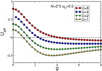
Figure 1: (Color online) Binding energy $U_{\rm eff}$ on a four site cluster as a function of the coupling $g$ to the dynamically fluctuating field $\sigma^{z}$. The binding energy $U_{\rm eff}$ can go negative at large $g$, suggesting the possibility of pairing.

In this paper we examine the properties of the dynamic Hubbard Hamiltonian with determinant Quantum Monte Carlo (DQMC)blankenbecler81 . This approach allows us to work in two dimensions, as opposed to previous ($d=1$) WLQMC studies, and also to examine lattices of an order of magnitude greater number of sites than ED. On the other hand, the ability of DQMC to reach low temperatures is limited by the sign problemloh90 . We find that the extended $s$-wave pairing vertex, which is repulsive in the static Hubbard model, is attractive in the dynamic model, that is, extended $s$-wave superconducting correlations are enhanced by the dynamic fluctuations. However, the pairing susceptibilities are still only rather weakly increasing down to the lowest temperatures accessible to us (temperature $T$ greater than 1/40 the electronic bandwidth).

We also find, near half-filling, that the antiferromagnetic correlations can be enhanced relative to the static Hubbard Hamiltonian, particularly for densities above $\rho=1$. The Mott gap can also be stabilized. Interestingly, the total energy appears to be close to linear in the particle density, as opposed to a clear concave up curvature in the static Hubbard model (with either repulsive or attractive interactions).

The organization of this paper is as follows: In the next section we present our computational method, DQMC, as it applies to the dynamic Hubbard model. We describe several minor adjustments to the DQMC algorithm for the static Hubbard model that are needed in order to study the dynamic model. Our observables are also defined. In Section III, we present the results from our Monte Carlo simulations. The topics of antiferromagnetism and the Mott transition, pair susceptibilities and superconductivity, and the energy characteristics of the dynamic Hubbard model are discussed. The paper closes with conclusions in Section IV.

II Computational Methods

Although he did not undertake such studies, Hirsch pointed out hirsch02 that the dynamic Hubbard model could be simulated with a relatively minor modification of the DQMC methodblankenbecler81 . In DQMC, an auxiliary ‘Hubbard-Stratonovich’ (HS) field is introduced to decouple the on-site Hubbard repulsion. The trace over the resulting quadratic form of fermion operators is performed analytically, leaving an expression for the partition function which is a sum over the HS variables whose weight is given by the product of two determinants, one for spin up and one for spin down, that are produced by evaluating the trace.

In DQMC for the usual Hubbard Hamiltonian, the HS field couples to the difference between the up and down spin electron densities, with a coupling constant which is independent of spatial site and imaginary time. In a simulation of the dynamic Hubbard model, the coupling of the HS field depends on the dynamic field $\sigma^{z}_{\bf{i}}(\tau)$. The imaginary time dependence arises from the transverse term $\sigma^{x}_{\bf{i}}$ in the Hamiltonian. When the path integral for the partition function is constructed $\sigma^{x}_{\bf{i}}$ induces flips between the two values $\sigma^{z}_{\bf{i}}=\pm 1$, so this quantity becomes dependent on $\tau$. As a consequence, minor modifications are required to the standard expressions blankenbecler81 for the ratio of determinants before and after the Monte Carlo move of a HS variable, and for the re-evaluation of the Green’s function.

The dynamic field variables must also be updated, and again, only minor modifications of the formulae for the determinant ratio and Green’s function update are required. A final difference is that there is a contribution to the weight coming from the $\sigma^{x}$ and $\sigma^{z}$ terms in the Hamiltonian. The former try to align the dynamic variables in the imaginary time direction, while the latter favor positive values of the dynamic field. Such pieces of the action, which enter the weight of the configuration along with the fermion determinants, are similar to those arising in simulations of the Holstein Hamiltonianniyaz93 .

We verified our DQMC code by comparing to exact diagonalization results on a 2x2 spatial lattice (Figs. 1,2), and also by checking analytically soluble limits such as $t=0$. The results of our DQMC/diagonalization calculations on 2x2 lattices are completely consistent with those of Hirsch. For example, we have quantitatively reproduced the binding energy plot, Fig. 1(top) of Ref. hirsch02, and our Fig. 1. As a further check, we compared DQMC results for the double occupancy, $\langle n_{\uparrow}n_{\downarrow}\rangle$, and the expectation value of the dynamic field, $\langle\sigma^{z}\rangle$, to results from ED. See Fig. 2.

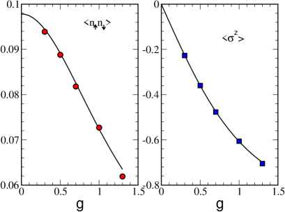
Figure 2: (Color online) Double occupancy (left) and expectation value of dynamic field (right) as functions of the coupling $g$. The solid line is the result of exact diagonalization and the symbols of the determinant QMC simulations. The cluster size is 2x2 (the same as for the binding energy calculation of Fig. 1 and Ref. hirsch02, ). Parameters are $t=1,\,U=4,\,\beta=1.3,\,\mu=2$ and $\omega_{0}=1.5$.

We did not observe any major difference in the characteristics of the DQMC algorithm in simulating the dynamic Hubbard model: Autocorrelation times remain short, as is typically the case with DQMC, and there was no major change in the numerical stability white89b ; sugiyama86 ; fye88 ; sorella89 . The key issue in DQMC is the ‘sign problem’ which we will discuss in the following sections.

DQMC allows us to measure any observable which can be expressed as an expectation value of products of creation and destruction operators. Our measurements include the energy $\langle H\rangle$ (not including the chemical potential term), particle density $\rho=\langle n\rangle$, and Green’s function $G_{\bf{ij}}(\tau)=\langle c_{\bf{i}}(\tau)c_{\bf{j}}^{\dagger}(0)\rangle$, as well as the average of the dynamic field $\langle\sigma^{z}_{\bf{i}}\rangle$. The dependence of the density on the chemical potential $\mu$ and the Green’s function, when analytically continued to the spectral function, allows us to examine, among other things, the Mott metal-insulator transition.

In addition to these single particle properties we also examine magnetic correlations, and specifically, the magnetic structure factor,

$$S({\bf k})=\sum_{{\bf l}}e^{i{\bf k}\cdot{\bf l}}\,\,\langle\,\,(n_{{\bf j+l}\uparrow}-n_{{\bf j+l}\downarrow})(n_{{\bf j}\uparrow}-n_{{\bf j}\downarrow})\,\,\rangle\,\,.$$ (2)

Our focus will be on the antiferromagnetic response, $S({\bf k}=(\pi,\pi))$.

We look at superconductivity by computing the correlated pair field susceptibility, $P_{\alpha}$, in different symmetry channels,

$$P_{\alpha} = \int_{0}^{\beta}d\tau\langle\Delta_{\alpha}(\tau)\Delta_{\alpha}^{\dagger}(0)\rangle$$

$$\Delta^{\dagger}_{\alpha} = {1\over N}\sum_{\bf k}f_{\alpha}({\bf k})c^{\dagger}_{{\bf k}\uparrow}c^{\dagger}_{-{\bf k}\downarrow}$$

$$f_{s}({\bf k}) = 1$$

$$f_{s^{*}}({\bf k}) = {\rm cos}(k_{x})+{\rm cos}(k_{y})$$

$$f_{d}({\bf k}) = {\rm cos}(k_{x})-{\rm cos}(k_{y})\,\,.$$ (3)

These quantities can also be expressed in real space,

$$\Delta^{\dagger}_{s} = {1\over N}\sum_{\bf i}c^{\dagger}_{{\bf i}\uparrow}c^{\dagger}_{{\bf i}\downarrow}$$

$$\Delta^{\dagger}_{s^{*}} = {1\over N}\sum_{\bf i}c^{\dagger}_{{\bf i}\uparrow}\Big{(}c^{\dagger}_{{\bf i}+\hat{x}\downarrow}+c^{\dagger}_{{\bf i}+\hat{y}\downarrow}+c^{\dagger}_{{\bf i}-\hat{x}\downarrow}+c^{\dagger}_{{\bf i}-\hat{y}\downarrow}\Big{)}$$

$$\Delta^{\dagger}_{d} = {1\over N}\sum_{\bf i}c^{\dagger}_{{\bf i}\uparrow}\Big{(}c^{\dagger}_{{\bf i}+\hat{x}\downarrow}-c^{\dagger}_{{\bf i}+\hat{y}\downarrow}+c^{\dagger}_{{\bf i}-\hat{x}\downarrow}-c^{\dagger}_{{\bf i}-\hat{y}\downarrow}\Big{)}\,\,.$$ (4)

The correlated susceptibility $P_{\alpha}$ takes the expectation value of the product of the four fermion operators entering Eq. 3. We also define the uncorrelated pair field susceptibility $\overline{P}_{\alpha}$ which instead computes the expectation values of pairs of operators prior to taking the product. Thus, for example, in the $s$-wave channel,

$$P_{s} = {1\over N^{2}}\sum_{{\bf i},{\bf j}}\int_{0}^{\beta}d\tau\langle\,c_{{\bf i}\downarrow}(\tau)\,c_{{\bf i}\uparrow}(\tau)\,c^{\dagger}_{{\bf j}\uparrow}(0)\,c^{\dagger}_{{\bf j}\downarrow}(0)\,\rangle$$

$$\overline{P}_{s} = {1\over N^{2}}\sum_{{\bf i},{\bf j}}\int_{0}^{\beta}d\tau\langle\,c_{{\bf i}\downarrow}(\tau)\,c^{\dagger}_{{\bf j}\downarrow}(0)\,\rangle\,\,\langle\,c_{{\bf i}\uparrow}(\tau)\,c^{\dagger}_{{\bf j}\uparrow}(0)\,\rangle\,\,.$$ (5)

$P_{\alpha}$ includes both the renormalization of the propagation of the individual fermions as well as the interaction vertex between them, whereas $\overline{P}_{\alpha}$ includes only the former effect. Indeed by evaluating both $P$ and $\overline{P}$ we are able to extract getgamma the interaction vertex $\Gamma$,

$$\Gamma_{\alpha}={1\over P_{\alpha}}-{1\over\overline{P}_{\alpha}}\,\,.$$ (6)

If $\Gamma_{\alpha}<0$, the associated pairing interaction is attractive. $\Gamma_{\alpha}\rightarrow-1$ signals a superconducting instability.

III Results

III.1 Mott Transition and Antiferromagnetism

It is useful to begin our study of the dynamic Hubbard model by understanding the behavior of the dynamic field at different fillings (Fig. 3). For fillings below one particle per site, $\rho<1$, the dynamic field $\sigma^{z}_{\bf{i}}\simeq-1$ because of the coupling to the external field$g\omega_{0}$ hence the interaction $U+2g\omega_{0}\simeq U_{\rm max}$ and the double occupancy is reduced. However, once double occupancy is unavoidable ($\rho>1)$, the interaction term strongly favors $\sigma^{z}_{\bf{i}}=+1$. Fig. 3 shows that this evolution from negative to positive values is nearly linear once $\rho>1$. Meanwhile, the expectation value of $\sigma^{x}_{\bf{i}}$ measures the fluctuations of $\sigma^{z}_{\bf{i}}$ in imaginary time. It is not surprising, then, that this quantity exhibits a maximum at roughly the midpoint between the evolution from $\sigma^{z}_{\bf{i}}=-1$ to $\sigma^{z}_{\bf{i}}=+1$, at $\rho\approx 1.5$. In the results of Fig. 3, and throughout this paper unless otherwise stated, the simulations were performed on 6x6 lattices.

Next, we compare the Mott gap and magnetic correlations in the static and dynamic Hubbard models. In Fig. 4 we plot the density $\rho$ as a function of chemical potential $\mu$. A plateau at $\rho=1$ indicates the formation of a Mott insulator. The cost to add a particle suddenly jumps by $U$ because additional particles are forced to sit on sites which are already occupied. At the inverse temperature chosen, $\beta=5$, for the static Hubbard model, the plateau is only beginning to develop. However for the dynamic model the plateau is much more robust. This is expected since near half-filling, as we have seen, the on-site repulsion mostly takes on its maximum value $U_{\rm max}=7.8$, for the parameters in Fig. 4. We have chosen dynamic Hubbard parameters $g$ and $\omega_{0}$ which gets the system as close as possible to the most attractive (negative) binding energy $U_{\rm eff}$ while still having $U_{\rm min}>0$.

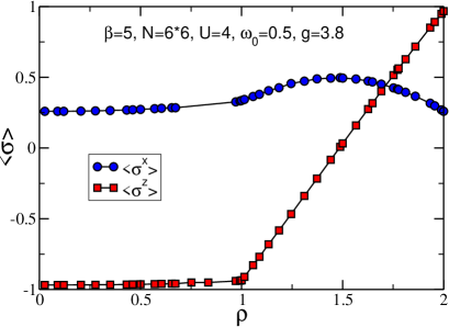
Figure 3: (Color online) $\langle\sigma^{z}\rangle$ and $\langle\sigma^{x}\rangle$ as a function of $\rho$ for $\omega_{0}=0.5,g=3.8$. From $\rho=0$ to half-filling, the system minimizes its energy by maximizing the interaction term $U-2g\omega_{0}\sigma^{z}$ to avoid double occupation, that is, $\langle\sigma^{z}\rangle\simeq-1$. In this Figure, and elsewhere in this paper, the lattice size is 6x6 unless otherwise stated.

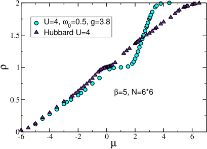
Figure 4: (Color online) Comparison of the evolution of the density $\rho$ with chemical potential $\mu$ for the static and dynamic Hubbard models. The dynamic model has a significantly better developed Mott insulating gap, as well as a pronounced particle-hole asymmetry. Here the inverse temperature $\beta=5$.

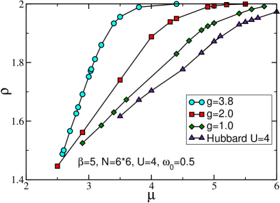
Figure 5: (Color online) The density $\rho$ as a function of chemical potential $\mu$ at $U=4$ and $\beta=5$. As the coupling $g$ increases, the cost to add particles to an already occupied site decreases. As a consequence, $\rho$ rises more steeply with $\mu$.

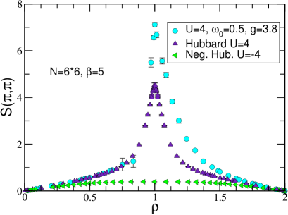
Figure 6: (Color online) The antiferromagnetic structure factor $S(\pi,\pi)$ at inverse temperature $\beta=5$ as a function of density $\rho$. For both the static and dynamic repulsive Hubbard Hamiltonians there is significant antiferromagnetic order near half filling, with the magnetic correlations in the dynamic model somewhat more robust. There is no magnetic signal for the attractive model which, instead, is known to show strong charge density wave and $s$-wave superconducting correlations.

Figure 5 gives further insight into the behavior of the density near full filling. In the static model, the cost to add particles to the system is set by the on-site $U$ (in the case that $U$ exceeds the bandwidth $W=8t$). However, in the dynamic model, as full filling is approached, the double occupancy cost is reduced to $U_{\rm min}$. For the parameters chosen in Fig. 5, $U_{\rm min}=0.2$ is close to zero. Thus we expect the filling of the lattice to be complete when the chemical potential reaches the top of the band, $4t$, in good agreement with the plot.

The static Hubbard model exhibits antiferromagnetic correlations at half-filling on a bipartite lattice, since only electrons with anti-aligned spins can hop between neighboring sites. This leads to a lowering of the energy by the exchange energy $J=4t^{2}/U$ relative to sites with parallel spin, for which hopping is forbidden. Indeed, a finite size scaling analysis of the structure factor has shown there is long range order in the ground statehirsch89 . Figure 6 compares the value of the antiferomagnetic structure factor $S(\pi,\pi)$ for the static and dynamic models. At half-filling, $S(\pi,\pi)$ for the dynamic model attains a maximal value 50% larger than that of the static model. There is a marked asymmetry in the magnetic response at values greater and lower than $\rho=1$ in the dynamic model, with $S(\pi,\pi)$ remaining high to values of $\rho$ ten percent larger than half-filling. We also show results for the negative $U$ Hubbard model, which has no tendency for magnetic order at any filling. (Instead, the attractive Hubbard model exhibits long range charge and superconducting correlations at $\rho=1$).

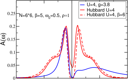
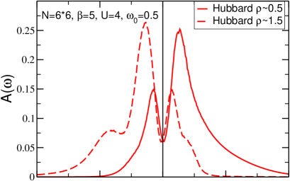
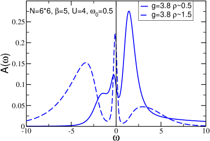
Figure 7: (Color online) Top: Comparison of the spectral function $A(\omega)$ for the static and dynamic Hubbard models at $\beta=5$ and half-filling. We can see clearly that the Mott gap is more robust in the dynamic case. Middle and bottom: The behavior of $A(\omega)$ away from half-fillingnote3 . In all cases the spectral function is finite at the Fermi energy, indicating metallic behavior. However, for the dynamic model at $\rho=1.5$ there is a sharp resonance at $\omega=0$ whereas in the other cases the spectral function is suppressed there.

The spectral function $A(\omega)$, which we obtain with an analytic continuation of $G(\tau)$ using the maximum entropy methodmaxent , shows supporting evidence for the enhancement of the Mott gap at half-filling, Fig. 7(top). Above half-filling $A(\omega)$ exhibits a sharp resonance at $\omega=0$, Fig. 7(bottom). The comparison of $A(\omega)$ for $\rho=0.5$ and $\rho=1.5$ further emphasizes the lack of particle-hole symmetry, Fig. 7(bottom).

III.2 Pairing Susceptibilities

We turn now to a discussion of superconductivity in the dynamic model. In the static Hubbard model, it has been shown that the $s$-wave pairing vertex is repulsive (positive). The $d$-wave vertex is negative, but only relatively weakly so at the temperatures accessible to the simulationswhite89 ; white89b . Near half-filling, the extended $s$-wave vertex is also attractive, but markedly less so than $d$-wave, suggesting that $d$-wave symmetry is the most likely instability. However, the same sign problem which precludes a definitive statement about superconductivity in the static model also limits what we can conclude here for the dynamic model. Nevertheless, there is an interesting qualitative difference between the two models which can be clearly discerned.

Specifically, the extended $s$-wave vertex is attractive in the dynamic model in the regime of $g$ where $U_{\rm eff}$ is negative, while it is repulsive in the static model at these high fillings. In Fig. 8 we compare the temperature evolution of the correlated and uncorrelated susceptibilities, $P_{s^{*}}$ and $\overline{P}_{s^{*}}$, at $\rho=1.89$ and $U=3$ and see that the $P_{s*}>\overline{P}_{s^{*}}$. The average sign takes the values 0.94, 0.92, 0.83, 0.73, and 0.63 at $\beta=5,6,7,8,9$ respectively. The resulting attractive (negative) vertex is given in Fig. 9. For $g=0$, the static model, the vertex is repulsive. But it systematically decreases and goes negative as the coupling to the dynamic field is strengthened. In this plot the inverse temperature is fixed at $\beta=5$ and the density is allowed to vary. The average sign takes the values 0.36, 0.54, 0.73, 0.89, and 0.96 at $\rho=1.50,1.60,1.70,1.80,1.90$.

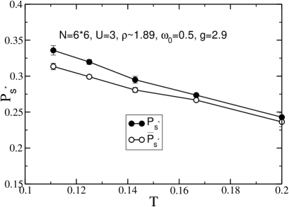
Figure 8: (Color online) The extended $s$-wave pair susceptibilities $P_{s}^{*}$ and $\overline{P}_{s^{*}}$ as a function of temperature for $U=3,\omega_{0}=0.5$, and $g=2.9$. Here, unlike the static model, $P_{s^{*}}$ exceeds $\overline{P}_{s^{*}}$ when the temperature is lowered. However, we cannot say if $P_{s^{*}}$ might diverge at low temperature because of the sign problem.

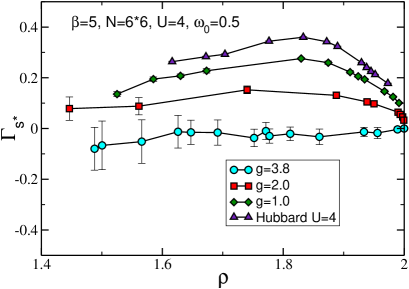
Figure 9: (Color online) $\Gamma_{s*}$ as a function of density $\rho$ for $\beta=5$ near full-filling. The $s^{*}$ channel becomes attractive when $g$ increases. $\Gamma_{s*}\rightarrow-1$ would signal a superconducting instability.

Figure 10 (top) shows that, in contrast to the behavior of $\Gamma_{s^{*}}$, the s-wave vertex is strongly repulsive, although $g$ does weaken the repulsion somewhat as it increases. Meanwhile, we see in Fig.10 (bottom) that near full filling the $d$-wave vertex is more weakly attractive than the $s^{*}$-wave vertex. This suggests that if the dynamic Hubbard model does have a superconducting instability at small hole-doping that it would be of $s^{*}$ symmetry, unlike the $d$-wave symmetry which is most attractive for the static modelnote2 .

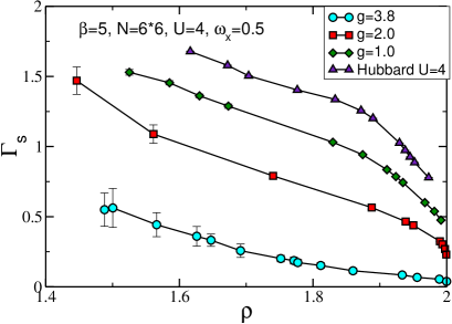
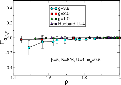
Figure 10: (Color online) Top: $\Gamma_{s}$ as a function of $\rho$ for different values of $g$ at $\beta=5$. Unlike $\Gamma_{s^{*}}$, the $s$-wave channel remains repulsive. Bottom: $\Gamma_{d_{x^{2}-y^{2}}}$ as a function of $\rho$. The $d_{x^{2}-y^{2}}$-wave channel is attractive, but the effect is less pronounced than for $s^{*}$, especially near full filling.

It is informative to compare the onset of attraction in the pairing vertex with the development of negative binding energy. Fig. 11 shows $\Gamma_{s},\Gamma_{s^{*}}$ and $\Gamma_{d_{x^{2}-y^{2}}}$ versus $g$ for $U=4$ and $\omega_{0}=0.5$. The filling $\rho=1.8$. On 2x2 lattices, for which the ED calculation of $U_{\rm eff}$ is feasible, $\Gamma_{s^{*}}$ becomes negative at somewhat larger values of $g$ than where $U_{\rm eff}$ becomes negative. The figure also shows that $\Gamma$ is relatively insensitive to lattice size: the 2x2 and 6x6 lattices give results which are quantitatively rather similar for most values of $g$. Note also that $\Gamma_{s^{*}}$ is strongly repulsive in the static model $g=0$.

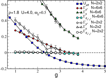
Figure 11: (Color online) Pairing vertices and binding energy as functions of the dynamical coupling $g$. $\Gamma_{s^{*}}$ becomes negative at $g>3.5$ while $U_{\rm eff}<0$ when $g>2.3$. As long as $g<4$, i.e. for the entire range of the horizontal axis, both $U_{\rm min}$ and $U_{\rm max}$ are repulsive. $\Gamma_{s^{*}}$ is strongly repulsive in the static model $g=0$.

A significantly larger enhancement of superconductivity was reported marsiglio90 in a Hubbard Hamiltonian in which the hopping of one spin species is modulated by the density of the other. This model was argued to be connected to the dynamic Hubbard Hamiltonian in the limit of large $w_{0}$. We conclude this section by exploring the $w_{0}$ dependence of the pairing vertex, to see if larger $w_{0}$ might show a greater tendency for superconductivity. In Fig. 12 we show the vertices as a function of $w_{0}$. We have fixed the product $gw_{0}=1.9$ and $U=4$ so we can stay near the values of $U_{\rm min}$ where the binding energy is maximized. The attraction does not seem to increase markedly with $w_{0}$.

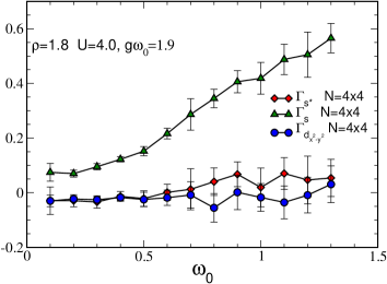
Figure 12: (Color online) Pairing vertices as functions of frequency $w_{0}$ at fixed $gw_{0}=1.9$, $\rho=1.8$, $\beta=5$, and $U=4$. The attractive d-wave vertex shows only a weak dependence on $w_{0}$.

III.3 Energy

The total energy (Fig.13) also shows a markedly different dependence on the density, $\rho$, in the dynamic Hubbard Hamiltonian. Whereas the static positive and negative $U$ Hubbard Hamiltonians have $d^{2}E/d\rho^{2}>0$, the positive curvature of the dynamic model that is evident below half-filling becomes very small for $\rho>1$ as $g$ increases and eventually the curvature nearly vanishes. Figure 14 shows this linear behavior developing with $g$.

The temperatures at which we performed our simulations are low enough that the total internal energy, $E$, is nearly equal to the free energy, $F$. As it is well known, negative curvature in the free energy as a function of the density, in the canonical ensemble, leads to negative compressibility and is thus a signal for phase separation and a first order phase transitionphasesep . Thermodynamic stability requires positive curvature for the free energy versus density. While our simulations are performed in the grand canonical ensemble, where such negative curvatures are not observed, we do see (Fig. 14) a progression from positive to zero curvature as $g\to 4$. At the same time, and recalling that $\mu=\partial(F/V)/\partial\rho$, we see in Fig. 5 that as $g\to 4$, the $\rho$ versus $\mu$ curves get steeper signalling higher compressibility $\kappa=\partial\rho/\partial\mu$. Noting that $U_{\rm min}$ vanishes for $g=4$ and becomes negative when $g>4$, we interpret these observations as a possible phase separation setting in at $g=4$ whereby the system develops hole-rich and hole-deficient regions.

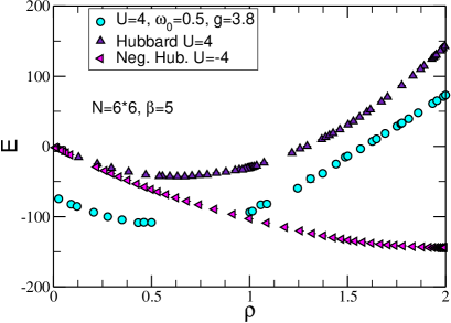
Figure 13: (Color online) Total energy as a function of $\rho$ at $\beta=5$ for the static attractive and repulsive Hubbard models, and for the dynamic model. The static models show clear positive curvature, indicative of thermodynamic stability. In the dynamic model $E(\rho)$ is nearly linear.

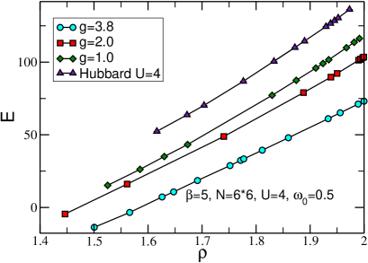
Figure 14: (Color online) Total energy as a function of $\rho$ at $\beta=5$. For $g=0$, the static model, the curvature is positive. As $g$ gets larger, the energy becomes linear in the density.

IV Conclusions

In this paper we have performed determinant Quantum Monte Carlo simulations of a two dimensional Hubbard Hamiltonian in which the on-site repulsion is coupled to a fluctuating bosonic field. Our studies complement earlier work using the Lang-Firsov transformation and exact diagonalization and QMC in one dimension. We note a number of interesting features of the model. First, the Mott gap at half-filling is stabilized. Second, antiferromagnetic correlations are enhanced above half-filling. The extended $s$-wave pairing vertex, which is repulsive in the ordinary static Hubbard Hamiltonian, is made attractive in the dynamic model. The value of $g$ for which this attraction manifests is roughly consistent with the value at which the binding energy $U_{\rm eff}$ goes negative on 2x2 clusters. The sign problem prevents simulations at low temperatures to see if an actual pairing instability occurs. We have also observed that as $g\to 4$, i.e. as $U_{\rm min}\to 0$, $E(\rho)$ becomes linear in $\rho$ signalling possible phase separation into regions of hole-deficient and hole-rich regions when $U_{\rm min}$ becomes negative for $g>4$. Finally, we note that we have also found, within the Hartree-Fock framework, that charge inhomogeneities (stripes) are supported by this dynamic Hubbard model bouadimunp .

KB, FH, and GGB acknowledge financial support from a grant from the CNRS (France) PICS 18796, RTS from NSF ITR 0313390, and ME from the Research Corporation. We acknowledge very useful help from M. Schram and R.Waters.

References

- (1) See, for example, Lecture Notes on Electron Correlation and Magnetism, Springer Series in Condensed Matter Physics Vol. 5, P. Fazekas, World Scientific (1999).
- (2) S.R. White, D.J. Scalapino, R.L. Sugar, N.E. Bickers, and R.T. Scalettar, Phys. Rev. B39, 839 (1989).
- (3) S.R. White, D.J. Scalapino, R.L. Sugar, E.Y. Loh, J.E. Gubernatis, and R.T. Scalettar, Phys. Rev. B40, 506 (1989).
- (4) C.C Tsuei and J.R. Kirtley, Phys. Rev. Lett. 85, 182 (2000).
- (5) E.Y. Loh, J.E. Gubernatis, R.T. Scalettar, S.R. White, D.J. Scalapino, and R.L. Sugar, Phys. Rev. B41, 9301 (1990).
- (6) Th. Maier, M. Jarrell, Th. Pruschke, and J. Keller, Phys. Rev. Lett. 85, 1524 (2000).
- (7) Thomas A. Maier, M. Jarrell, and D. J. Scalapino, Phys. Rev. B74, 094513 (2006).
- (8) D. Poilblanc and T.M. Rice, Phys. Rev. B39, 9749 (1989); J. Zaanen and O. Gunnarsson, Phys. Rev. B40, 7391 (1989); and B. Normand and A. P. Kampf, Phys. Rev. B64, 024521 (2001).
- (9) U.Schollwock, Rev. Mod. Phys. 77, 259 (2005).
- (10) J.M. Tranquada, B.J. Sternlieb, J.D. Axe, Y. Nakamura and S. Uchida, Nature 365, 561 (1995); and T. Noda, H. Eisaki and S. Uchida, Science 286, 265 (1999).
- (11) V.J. Emery, Phys. Rev. Lett, 58, 2794 (1987).
- (12) F. C. Zhang and T. M. Rice, Phys. Rev. B37, 3759 (1988).
- (13) A. Lanzara, P.V Bogdanov, X.J. Zhou, S.A Kellar, D.L. Feng, E.D. Lu, T. Yoshida, H. Eisaki, A. Fujimori, K. Kishio, J.-I. Shimoyama, T. Noda, S. Uchida, Z.Hussain and Z.-X. Shen, Nature 412, 510 (2001).
- (14) J.E. Hirsch, Phys. Rev. Lett. 87, 206402 (2001).
- (15) J.E. Hirsch, Phys. Rev. B65, 214510 (2002).
- (16) J.E. Hirsch, Phys. Rev. B66, 064507 (2002).
- (17) J.E. Hirsch, Phys. Rev. B67, 035103 (2003).
- (18) F. Marsiglio, R. Teshima, and J.E. Hirsch, Phys. Rev. B68, 224507 (2003).
- (19) Actually, J.E Hirsch originally proposed a modulation of the on-site repulsion with a coupling to a continuous bosonic mode, . In later papers he argued for the equivalence to a model with a discrete (Ising-like) degree of freedom.
- (20) J.E. Hirsch, R.L. Sugar, D.J. Scalapino and R. Blankenbecler, Phys. Rev. B26, 5033 (1982).
- (21) R. Blankenbecler, R.L. Sugar, and D.J. Scalapino, Phys. Rev. D24, 2278 (1981).
- (22) P. Niyaz, J.E. Gubernatis, R.T. Scalettar, and C.Y. Fong, Phys. Rev. B48, 16011 (1993).
- (23) G. Sugiyama and S.E. Koonin, Ann. Phys. 168, 1 (1986).
- (24) R.M. Fye and J.E. Hirsch, Phys. Rev. B38, 433 (1988).
- (25) S. Sorella, S. Baroni, R. Car, and M. Parrinello, Europhys. Lett. 8, 663 (1989); and S. Sorella, E. Tosatti, S. Baroni, R. Car, and M. Parrinello, Int. J. Mod. Phys. B1, 993 (1989).
- (26) R.T. Scalettar, D.J. Scalapino, R.L. Sugar and S.R. White, Phys. Rev. B44, 770 (1991).
- (27) J. E. Hirsch and S. Tang, Phys. Rev. Lett. 62, 591 (1989).
- (28) J.E Gubernatis, M. Jarell, R.N. Silver and D.S. Sivia, Phys. Rev B44, 6011 (1991).
- (29) In the static Hubbard case, Fig. 7(middle), the densities are and which is one cause of the slight asymmetry.
- (30) We comment that the attraction exhibited in the -wave vertex of the static model is most manifest at half-filling, where the cuprates are antiferromagnetic insulators. This is possibly, however, a consequence of small lattice size since then the pair creation operator which adds two particles to the system, significantly shifts the density.
- (31) F. Marsiglio and J.E. Hirsch, Physica C171, 554 (1990).
- (32) G. G. Batrouni and R. T. Scalettar, Phys. Rev. Lett. 84, 1599 (2000).
- (33) K. Bouadim, unpublished.