Emergent Symmetry and Dimensional Reduction at a Quantum Critical Point

Abstract

We show that the spatial dimensionality of the quantum critical point associated with Bose–Einstein condensation at $T=0$ is reduced when the underlying lattice comprises a set of layers coupled by a frustrating interaction. For this purpose, we use an heuristic mean field approach that is complemented and justified by a more rigorous renormalization group analysis. Due to the presence of an emergent symmetry, i.e. a symmetry of the ground state that is absent in the underlying Hamiltonian, a three–dimensional interacting Bose system undergoes a chemical potential tuned quantum phase transition that is strictly two dimensional. Our theoretical predictions for the critical temperature as a function of the chemical potential correspond very well with recent measurements in BaCuSi₂O₆.

I Introduction

The universal properties that appear in the proximity of a critical point are determined by a few relevant properties. The spatial dimensionality, $d$ , is one of them Stanley . This is evident from the fact that, in general, the critical exponents depend on $d$. Correspondingly, for strongly anisotropic systems of weakly coupled chains or planes, critical behavior characteristic for $d=1$ or $d=2$ respectively can be observed beyond a certain distance from the critical point. The critical behavior crosses over to three–dimensional only in the close vicinity of the critical point of such anisotropic systems.

In contrast to this conventional dimensional crossover, the spatial dimensionality can be effectively reduced under certain conditions as the system approaches the critical point. This phenomenon of dimensional reduction is closely related to the notion of “ emergent sliding symmetries” Batista04 . Those are physical systems for which new symmetry transformations appear at low energies (in some cases only at $T=0$). In other words, the low energy spectrum of the system Hamiltonian is invariant under these symmetries but the whole spectrum is not Batista05 . We call these transformations “emergent symmetries” because they only appear at low energies. By “sliding symmetry” Zohar05 we mean symmetry transformations that only change a subset of the degrees of freedom which occupy a region of dimension lower than $d$. For instance, if our system is a 3D quantum magnet and it is invariant under a spin rotation restricted to a given layer, such operation is a “sliding symmetry”.

A simple example of an emergent sliding symmetry is provided by classical spins on a body centered tetragonal (BCT) lattice with antiferromagnetic XY exchange interactions. If the inter–layer exchange interaction, $J_{\perp}$ , is smaller than the intra–layer one, $J_{\parallel}$, the energy is minimized when the spins are antiferromagnetically aligned on each layer. Since the staggered magnetization of each layer can point in any arbitrary direction, the ground state manifold is highly degenerate. In this case, an arbitrary spin rotation along the z–axis which acts only on the spins of a given layer is a sliding emergent symmetry. It is a symmetry because it does not change the ground state energy. It is “emergent” because it only exists at $T=0$: the energy does not remain invariant if we apply the same transformation to an excited state. In particular, this symmetry is the manifestation of a simple physical property: the order parameters (staggered magnetization) of different layers are decoupled at zero temperature. Consequently, in spite of the 3D nature of the system, the antiferromagnetic ordering is 2D at $T=0$ . This is a simple example of dimensional reduction that results from two key ingredients: the classical nature of the degrees of freedom and the frustrated nature of the interactions.

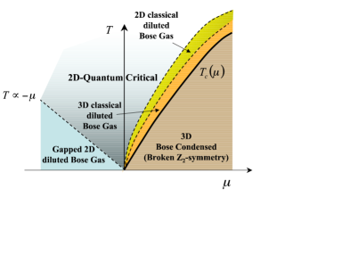
Figure 1: Phase diagram obtained by the renormalization group approach.

It is natural to ask if the phenomenon of dimensional reduction also exists in quantum systems. In most of the cases, the emergent sliding symmetry is removed by zero point fluctuations. For instance, if we consider now the quantum version of the XY model on a BCT lattice with $J_{\parallel}>J_{\perp}$, the ground state is no longer invariant under spin rotations along the z–axis of all the spins on a given layer. Therefore, this operation is an emergent symmetry only in the classical limit. Zero point fluctuations remove this symmetry by inducing a finite coupling between the staggered magnetization on different layers Maltseva05 ; Yildirim96 . This is a particular example of the phenomenon known as “order from disorder Shender82 .

However, zero point fluctuations not always restore the dimensionality by removing the emergent sliding symmetries. Such symmetries can appear at special points of the quantum phase diagram and lead to dimensional reduction. The main characteristic of these special points is that the ground state becomes “classical”, i.e., it is a direct product of eigenstates of a local physical operator. For instance, the fully polarized ferromagnet is a “classical” state for any spin $S$. A simple example of dimensional reduction in a quantum system is given in Ref.Batista004 for a Klein model of S=1/2 spins on square lattice. In that case, the dimensional reduction from $d=2$ to $d=1$ occurs at a first order quantum phase transition point. An immediate physical consequence of this dimensional reduction is the emergence of fractional excitations characteristic of one–dimensional systems.

We have shown recently that the phenomenon of dimensional reduction can also occur at a quantum critical point (second order quantum phase transition) Batista07 . For this purpose, we considered the quantum XY magnet of our previous example but in the presence of an external magnetic field, $H$, along the Z–direction. The ground state is antiferromgnetic for $H=0$ while the Zeeman term dominates at high fields leading to a fully polarized ground state. The antiferromagnetically ordered XY component decreases continuously as a function of $H$ and vanishes at the critical field $H_{c}$. The spin system becomes fully polarized for $H>H_{c}$. The corresponding quantum phase transition is denoted as Bose–Einstein condensation (BEC) because the order is suppressed by suppressing the amplitude of the order parameter or staggered magnetization. In contrast, the thermodynamic phase transition is denoted as XY because the order is suppressed by phase fluctuations. As we will see below, this difference is crucial for the phenomenon of dimensional reduction. The BEC–QCP of the system under consideration has a peculiar property: the disordered state for $H>H_{c}$ is “classical” because it is a direct product of eigenstates of $S_{i}^{z}$ ($z$–component of the spin operator on a given site $i$). In other words, the zero point phase fluctuations that restore the 3D ordering at $H=0$ are no longer present for $H>H_{c}$ simply because the XY spin component has been suppressed completely. Since the transition is continuous, the 3D coupling induced by these phase fluctuations must vanish continuously when $H$ approaches $H_{c}$ from the ordered side. For this reason, dimensional reduction occurs right at the critical point.

The specific motivation for the theory presented in this paper is the unusual temperature dependence of the transition temperature as function of magnetic field in frustrated magnet BaCuSi₂O₆Suchitra06 . We describe this system by a Heisenberg Hamiltonian of $S=$ $\frac{1}{2}$ spins forming dimers on a body–centered tetragonal lattice, closely approximating the case of BaCuSi₂O₆ Sparta04 ; Samulon06 . The dominant Heisenberg interaction, $J\sum_{\mathbf{i}}\mathbf{s}_{i1}\cdot\mathbf{s}_{i2}$, is between spins on the same dimer $i$. Since there are two low energy states in an applied magnetic field, the singlet and the $s_{i1}^{z}+s_{i2}^{z}=1$ triplet, we can describe the low energy sector either using hard–core bosons, or, in terms of the above mentioned XY model. In case of the hard core boson description, the triplet state corresponds to an effective site $i$ occupied by a boson while the singlet state is mapped into the empty site Giamarchi99 ; Jaime04 . The number of bosons (number of triplets) equals the magnetization along the $z$–axis. The chemical potential $\mu=g\mu_{B}(H-H_{c1})$ is determined by the applied magnetic field, $H$, and the critical field $g\mu_{B}H_{c1}=J-2J^{\prime}$ (where $g$ is the gyromagnetic factor, $\mu_{B}$ is the Bohr magneton and $J^{\prime}$ is the inter–dimer exchange interaction). The hoppings $t_{\parallel}=J^{\prime}$ and $t_{\perp}=J^{\perp}$ ($J^{\perp}$ is the frustrated inter–layer exchange interaction) are determined by the inter–dimer exchange interactions between spins. Recently, it was shown by Rösch and Vojta Rosch ; Rosch2 that the inclusion of the two higher triplet modes generates a small coherent second neighbor hopping of low energy triplets between layers $t_{\perp,2}^{\ast}\simeq J_{\perp}^{6}/J^{5}$. This interesting effect restores the $d=3$ character of the spin problem due to the fact that the paramagnetic ground state for $H<H_{c1}$ is not purely classical. Although it can be described as classical state (direct product of singlets on each dimer) to a very good approximation, there are small zero–point phase fluctuations that result from virtual process to the higher triplet states (creation and annihilation of triplet pairs with zero net magnetic moment). It was also pointed out in Refs.Rosch ; Rosch2 that the dimensional reduction is still exact at $H=H_{c2}$ (saturation field) because the state for $H>H_{c2}$ is purely classical. For realistic values of $J=49.5(1)$K and $J_{\perp}<J^{\prime}$, $J_{\perp}^{6}/J^{5}<0.1$mK in BaCuSi₂O₆. This implies that the mechanism discussed in our paper is still dominant for all experimentally accessible temperatures $T\gtrsim 30$mK. Moreover, the U(1)-symmetry breaking terms induced by dipolar interactions will produce a crossover to QCP with discrete symmetry at $T\sim 10$mK Suchitra006 before the mechanism of Ref.Rosch sets in. Finally, the inevitable presence of finite non-frustrated couplings in real systems will eventually restore the $d=3$ behavior below some characteristic temperature $T_{0}<30$mK.

Despite the above mentioned effects, where lattice distortions, dipolar couplings or excitations to high energy triplets cause a restoration of three dimensional behavior at very low temperatures, is it important to stress that the boson model discussed in this paper is a nontrivial interacting many-body system where the dimensional reduction at the $T=0$ quantum critical point is exact. Materials that can be described in terms of a chemical potential tuned Bose-Einstein Condensation on a frustrating lattice are then candidates for the dimensional reduction as caused by an emergent symmetry in the problem. In this sense are the conclusions of our paper are not limited to BaCuSi₂O₆ alone.

The main purpose of the present work is to derive the critical properties of the field induced BEC–QCP for the XY magnet mentioned above. The key finding of our result is the detailed phase diagram of Fig.1, where we show the various crossover regimes of a chemical potential tuned BEC on a frustrated lattice. This work complements the results presented in Ref.Batista07 by including a renormalization group approach (Sec. IV) which provides formal justification for the heuristic mean field approach presented in Ref.Batista07 and is summarized in detail in Section III. The model for the XY-magnet on a BCT lattice is introduced in Sec. II. For practical reasons, we use the language of hard core bosons which are equivalent to $S=1/2$ spins after a Matsubara–Matsuda transformation Matsubara56 . Our conclusions are presented in Section IV.

II Model

We start from the Hamiltonian of interacting spinless bosons on a body centered cubic lattice

$$H_{B}=\sum_{\mathbf{k}}\left(E_{\mathbf{k}}-\mu\right)a_{\mathbf{\ k}}^{\dagger}a_{\mathbf{k}}+u\sum_{i}n_{i}n_{i}.$$ (1)

Here $n_{i}=a_{i}^{\dagger}a_{i}$ is the local number operator of the bosons and

$$a_{\mathbf{k}}^{\dagger}=\frac{1}{\sqrt{N}}\sum_{i}a_{i}^{\dagger}e^{i\mathbf{\ k\cdot R}_{i}},$$ (2)

the corresponding creation operator in momentum space. The tight binding dispersion for nearest neighbor boson hopping on the BCT lattice is

$$E_{\mathbf{k}}=\varepsilon_{\mathbf{k}_{\parallel}}+2t_{\perp}\gamma_{\mathbf{k}_{\parallel}}\cos k_{z}c,$$ (3)

$\mathbf{k}_{\parallel}=\left(k_{x},k_{y}\right)$ refers to the in plane momentum and

$$\varepsilon_{\mathbf{k}_{\parallel}}=t_{\parallel}\left(2+\cos k_{x}a+\cos k_{y}a\right)$$ (4)

is the in-plane dispersion. For convenience we included the constant shift $2t_{\parallel}$ in the definition of $\varepsilon_{\mathbf{k}_{\parallel}}$ to ensure that $\varepsilon_{\mathbf{k}_{\parallel}}\geq 0$. The last term in Eq.(3) refers to the inter-plane coupling, where the form factor

$$\gamma_{\mathbf{k}_{\parallel}}=\cos\frac{k_{x}a}{2}\cos\frac{k_{y}a}{2}$$ (5)

describes the $\mathbf{k}_{\parallel}$-dependence of this coupling in the BCT lattice. This $\mathbf{k}_{\parallel}$-dependence is a crucial aspect of our theory.

For $t_{\parallel}$, $t_{\perp}>0$ and $t_{\parallel}>t_{\perp}/2$, Bose Einstein condensation takes place at $\mathbf{Q}=\left(\pi/a,\pi/a,k_{z}\right)$. Since $\gamma_{\mathbf{k}_{\parallel}}$ vanishes for $\mathbf{k}_{\parallel}=\left(\pi/a,\pi/a\right)$, $E_{\mathbf{Q}}$ is independent of $k_{z}$. The minimum of the dispersion is infinitely degenerate as the $z$-component of the wave vector can take any value when the $x$ and $y$ components are equal to $\pi/a$. In case of the ideal Bose gas ($u=0$) this implies for $T=0$ that different layers decouple completely. Only excitations at finite $T$ with in-plane momentum away from the condensation point can propagate in the $z$-direction. This behavior changes as soon as boson-boson interactions ($u>0$) are included. States in the Bose condensate scatter and create virtual excitations above the condensate that are allowed to propagate in the $z$-direction. These excitations couple to condensate states in other layersMaltseva05 . The condensed state of interacting bosons is then truly three dimensional, even at $T=0$. This order by disorder argument for dimensional restoration due to interactions does not apply in case of chemical potential tuned BEC. In this case, the number of bosons at $T=0$ is strictly zero for $\mu<0$, i.e. before BEC sets in. The absence of particles makes their interaction mute and one can approach the QCP arbitrarily closely without coherently coupling different layers.

From now on, we will measure the momentum relative to the wave vector $\mathbf{Q}_{0}=(\pi/a,\pi/a,0)$: $\mathbf{q}=\mathbf{k}-\mathbf{Q}_{0}$, such that BEC corresponds to a macroscopic occupation of a state with vanishing in-plane momentum, $\mathbf{q}_{\parallel}=0$. Since we will treat the inter-layer hopping, $t_{\perp}$, pertubativly, it is convenient to rewrite $H_{B}$ using real space variables for the direction perpendicular to the planes.

$$H_{B} = \sum_{\mathbf{q}_{\parallel},i}(\varepsilon_{\mathbf{q}_{\parallel}}-\mu)a_{\mathbf{q}_{\parallel}i}^{\dagger}a_{\mathbf{q}_{\parallel}i}^{\;}+u\sum_{\mathbf{x}_{\parallel},i}n_{\mathbf{x}_{\parallel}i}n_{\mathbf{x}_{\parallel}i}$$ (6)

$$+ t_{\perp}\!\!\!\sum_{\mathbf{q}_{\parallel},ij}\gamma_{\mathbf{q}_{\parallel}}\eta_{ij}(a_{\mathbf{q}_{\parallel}i}^{\dagger}a_{\mathbf{q}_{\parallel}j}^{\;}+h.c.),$$

The indices $i$,$j$ denote the different layers, with $\eta_{i,j}=1$ for nearest neighbor layers while $\eta_{i,j}=0$ otherwise. Due to the shift of momentum it holds

$$\gamma_{\mathbf{q}_{\parallel}}=\sin\frac{q_{x}}{2}\sin\frac{q_{y}}{2}.$$ (7)

We note that $H_{B}$ has a discrete $Z_{2}$–symmetry Maltseva05 ; Rosch ; Rosch2 :

$$q_{x} \rightarrow -q_{x},$$

$$a_{\mathbf{x}_{\parallel},i}^{\dagger} \rightarrow \left(-1\right)^{i}a_{\mathbf{x}_{\parallel},i}^{\dagger}.$$ (8)

for all $i$. This is a local $Z_{2}$–symmetry with respect to the layer index. In momentum space  the last equation corresponds to $q_{z}\rightarrow q_{z}+\pi/c$. The in-plane dispersion and the local interaction trivially obey this symmetry. However, the inter-layer hopping is only invariant with respect to this transformation since $\gamma_{\mathbf{q}_{\parallel}}$ is odd  with respect to either $q_{x}$ or $q_{y}$ . This discrete symmetry is therefore closely connected to the degeneracy of the Bose condensate with respect to $q_{z}$. If we were to include an additional inter-layer hopping term between neighboring planes with $\mathbf{\ q}_{\parallel}$-independent hopping $t_{1}$,

$$T_{1}=t_{1}\sum_{\mathbf{q}_{\parallel},ij}\eta_{ij}(a_{\mathbf{q}_{\parallel}i}^{\dagger}a_{\mathbf{q}_{\parallel}j}^{\;}+h.c.),$$ (9)

we would break the $Z_{2}$-symmetry. In addition we would lift the degeneracy of the Bose condensate to either $k_{z}=\pi/c$ or $k_{z}=0$, depending on the sign of $t_{1}$. On the other hand, inclusion of a term

$$T_{2}=t_{2}\sum_{\mathbf{q}_{\parallel},ij}\widetilde{\eta}_{ij}(a_{\mathbf{q}_{\parallel}i}^{\dagger}a_{\mathbf{q}_{\parallel}j}^{\;}+h.c.),$$ (10)

that promotes boson hopping between second neighbors ($\widetilde{\eta}_{i,i+2}=\widetilde{\eta}_{i+2,i}=1$ and $\widetilde{\eta}_{i,j}=0$ otherwise) would lift the degeneracy of the bose condensate, but without breaking the $Z_{2}$-symmetry. We will see below that this leads to important distinction between coherent coupling between nearest and next nearest neighbor layers.

While the Bose condensed state for $\mu>0$ and the entire regime for $T>0$ is three dimensional, the decoupling for $\left(\mu<0,T=0\right)$ has dramatic consequences. We show that the BEC transition temperature varies as

$$T_{c}\propto\mu\ln\left(\frac{t_{\parallel}}{\mu}\right)/\ln\ln\frac{t_{\parallel}}{\mu}.$$ (11)

$T_{c}$ $\propto\mu^{2/d}$ holds instead for an isotropic Bose system in $d>2$. Despite the fact that different layers are coupled at finite $T$ the BEC-transition temperature, Eq.(11), depends on $\mu$ just like the Berezinskii-Kosterlitz-Thouless (BKT) transition temperature of a two dimensional system FisherHohenberg88 .

The renormalization group (RG) calculation used to obtain this result (a one-loop RG calculation in analogy to Ref.FisherHohenberg88 ; Sachdev94 ) shows that the finite temperature transition is a classical $3$-$d$ $XY$ transition, not a BKT transition. We conclude, therefore, that the $T=0$ QCP of chemical potential tuned BEC with three dimensional dispersion, Eq.(3), is strictly two dimensional. The system then crosses over to be three dimensional for $\mu>0$ or $T>0$, where the density of bosons becomes finite and boson-boson interactions drive the crossover to $d=3$. The transition temperature of this three dimensional BEC is given by the two-dimensional result, Eq.(11). It is important to stress that the vanishing density for $\left(\mu<0,T=0\right)$ implies that these results are not limited to weakly interacting bosonsSachdev .

III Mean Field Theory

III.1 Phase Boundary

Here we present a heuristic derivation of Eq.(11) based on an approach introduced by Popov Popov83 and further explored by Fisher and Hohenberg FisherHohenberg88 : infrared divergencies are cut-off for momenta $q<q_{0}\simeq\sqrt{\mu/t_{\parallel}}$, where $\mu$ is the chemical potential. The main results of this approach were already given in Ref.Batista07 . We will show how an effective coupling along the $z$ –axis appears when the interaction term of $H_{B}$ is taken into account. For this purpose, we will approach the BEC-QCP from the disordered phase. Since we are interested in the case of hard-core bosons, we will consider an infinitely large on–site repulsive interaction $u\rightarrow\infty$.

While the interaction is local, scattering processes between bosons in different layers generate effective non-local interactions at low energies of the type

$${H_{\mathrm{int}}}=\frac{1}{2}\sum_{ijkl,\mathbf{x}_{\parallel}}v_{ijkl}(\mathbf{x}_{\parallel})a_{\mathbf{x}_{\parallel}i}^{\dagger}a_{{\mathbf{x}}_{\parallel}j}^{\dagger}a_{\mathbf{x}_{\parallel}k}^{\;}a_{\mathbf{x}_{\parallel}l}^{\;}.$$ (12)

To leading order in the boson density $\rho$, the Fourier transform $v_{0}(\mathbf{q}_{\parallel})\equiv v_{iiii}(\mathbf{q}_{\parallel})$ of the intra–layer effective interaction results from adding the ladder diagrams shown in Fig.2a Beliaev :

$$\frac{1}{v_{0}(\mathbf{q}_{1\parallel}+\mathbf{q}_{2\parallel})}=\frac{1}{4}\int\frac{d^{2}q_{\parallel}}{4\pi^{2}}\frac{1}{\varepsilon_{\mathbf{\ q}_{\parallel}+{\mathbf{q}_{1\parallel}}}+\varepsilon_{{\mathbf{q}_{2\parallel}-\mathbf{q}_{\parallel}}}},$$ (13)

where

$$\varepsilon_{{\mathbf{q}_{\parallel}}}=t_{\parallel}(2-\cos{q_{x}a}-\cos{q_{y}a})$$ (14)

due to the shift of the in-plane momentum. The integral in Eq.(2 ) diverges logarithmically in two dimensions for $\mathbf{q}_{1\parallel},\mathbf{q}_{2\parallel}\rightarrow 0$. The effective interaction will be logarithmically small in the low density limit. An heuristic way of deriving a consistent mean field theory is to introduce the cut-off $q_{0}\sim\sqrt{\mu/t_{\parallel}}$ Schick71 ; Popov83 ; FisherHohenberg88 :

$$\frac{1}{v_{0}}=\frac{1}{4}\int_{q_{0}}^{\pi}\frac{d^{2}q_{\parallel}}{4\pi^{2}}\frac{1}{\epsilon_{\mathbf{q}_{\parallel}}}\propto\frac{\ln{\ \frac{t_{\parallel}}{\mu}}}{t_{\parallel}}.$$ (15)

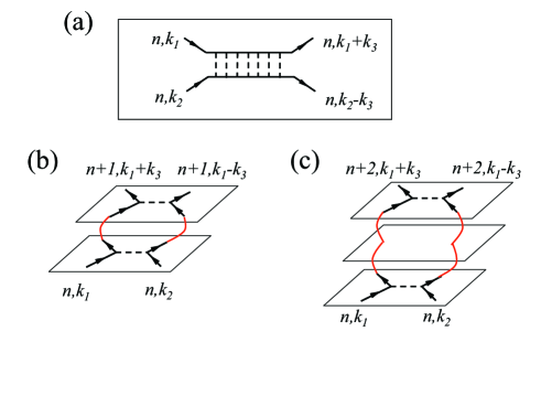
Figure 2: (a) Ladder diagrams that provide the dominant contribution to the intra–layer scattering in the low density regime Beliaev . (b) and (c) leading order diagrams that contribute to the coherent inter–layer hoppings $t_{\perp,1}^{\ast}$ and $t_{\perp,2}^{\ast}$.

We proceed now to compute the inter-layer interactions  $v_{ijkl}$ that are generated by combining the intra–layer renormalized interaction, $v_{0}$, with the inter-layer hopping term $t_{\perp}$. For this purpose, it is convenient to expand the propagator in powers of the inter–layer hopping:

$$G_{ij}(q_{\parallel}) = g(q_{\parallel})\delta_{ij}+t_{ij}(q_{\parallel})g^{2}(q_{\parallel})$$ (16)

$$+\sum_{l}t_{il}(q_{\parallel})t_{lj}(q_{\parallel})g^{3}(q_{\parallel})+...,$$

where $t_{ij}(\mathbf{q}_{\parallel})=t_{\perp}\gamma_{\mathbf{q}_{\parallel}}\eta_{i,j}$ and

$$g(q_{\parallel})=\frac{1}{-i\omega_{n}+\frac{t_{\parallel}}{2}q_{\parallel}^{2}-\mu}.$$ (17)

is the intra–layer propagator for long wavelengths ($q_{\parallel}\ll 1$). From now on, we  measure in plane momenta in units of $2\pi/a$ where $a$ is the in-plane lattice constant (i.e. we set $a=1$) and  work in the long wavelength limit $q_{\parallel}\ll 1$. The leading order inter-layer effective interactions that are relevant for inducing coherency along the $z$ -axis are $v_{iijj}\equiv v_{|i-j|}$ for $|i-j|=1$ (see Fig.2b) and $|i-j|=2$ (see Fig.2c). Analyzing the corresponding ladder diagrams yields:

$$v_{1}(p) = -v_{0}^{2}t_{\perp}^{2}\!\!\int\frac{d\omega d^{2}q}{\left(2\pi\right)^{3}}\gamma_{q}\gamma_{p-q}g^{2}(\ q)g^{2}(p-q),$$

$$v_{2}(p) = -v_{0}^{2}t_{\perp}^{4}\!\!\int\frac{d\omega d^{2}q}{\left(2\pi\right)^{3}}\gamma_{q}^{2}\gamma_{p-q}^{2}g^{3}(q)g^{3}(p-q).$$

Performing the momentum and frequency integration with lower momentum cut off $q_{0}$ and setting $p\rightarrow 0$ yields

$$v_{1} = -\frac{v_{0}^{2}t_{\perp}^{2}}{8\pi t_{\parallel}^{3}}\ln{\frac{\pi}{q_{0}},}$$

$$v_{2} = -\frac{9v_{0}^{2}t_{\perp}^{4}}{128\pi t_{\parallel}^{5}}\ln{\ \frac{\pi}{q_{0}}.}$$ (18)

The $v_{0}$, $v_{1}$ and $v_{2}$ processes generate the minimal number of terms that have to be included in the low energy effective Hamiltonian in order to provide a correct description of the critical properties of our bosonic system in the low density limit. The expression for the new interaction term in the low energy theory is

$${H_{\mathrm{int}}}=\frac{1}{2}\sum_{\mathbf{x}_{\parallel}ij}\sum_{m=0}^{2}v_{m}\delta_{\left|i-j\right|,m}\ a_{\mathbf{x}_{\parallel}i}^{\dagger}a_{\mathbf{x}_{\parallel}i}^{\dagger}a_{\mathbf{\ x}_{\parallel}j}a_{\mathbf{x}_{\parallel}j}.$$ (19)

The  $m=0$ term corresponds to intra–layer scattering vertex $v_{0}$. The other terms with $m=1$, $2$ describe hopping of pairs of bosons from the layer $i$ to the layer $j\pm m$. Now we perform the mean field decoupling (we suppress the in-plane coordinate $\mathbf{x}_{\parallel}$ for simplicity)

$$n_{i}n_{i} \simeq 2\rho n_{i}-\rho^{2},$$

$$a_{i}^{\dagger}a_{i}^{\dagger}a_{j}a_{j} \simeq a_{i}^{\dagger}a_{j}^{\;}\langle a_{i}^{\dagger}a_{j}^{\;}\rangle+a_{i}^{\dagger}a_{j}^{\;}\langle a_{i}^{\dagger}a_{j}^{\;}\rangle-\langle a_{i}^{\dagger}a_{j}^{\;}\rangle^{2},$$

where $\rho=\langle n_{\mathbf{x}_{\parallel},i}\rangle$. With this mean field approximation we obtain an effective single particle Hamiltonian  with dispersion

$$E_{\mathbf{q}}^{\ast}=E_{\mathbf{q}}+2v_{1}\kappa_{1}\cos{q_{z}}+2v_{2}\kappa_{2}\cos{2q_{z},}$$ (20)

with

$$\kappa_{j}=\int\frac{d^{2}q_{\parallel}}{4\pi^{2}}\left\langle a_{\mathbf{q}_{\parallel},i}^{\dagger}a_{\mathbf{q}_{\parallel},i+j}^{\;}\right\rangle,$$ (21)

and effective chemical potential

$$\mu^{\ast}=\mu-v_{0}\rho.$$ (22)

The mean values $\langle a_{\mathbf{q}_{\parallel},i}^{\dagger}a_{\mathbf{\ q}_{\parallel},i+j}^{\;}\rangle$ are given by:

$$\left\langle a_{\mathbf{q}_{\parallel},i}^{\dagger}a_{\mathbf{q}_{\parallel},i+j}^{\;}\right\rangle=\int_{-\pi}^{\pi}\frac{dq_{z}}{2\pi}\frac{\cos{(jq_{z})}}{e^{\beta\left(E_{\mathbf{q}}^{\ast}-\mu^{\ast}\right)}-1}.$$

It follows $\langle a_{\mathbf{q}_{\parallel},i}^{\dagger}a_{\mathbf{q}_{\parallel},i+1}^{\;}\rangle=0$, a result that is a consequence of the local $Z_{2}$ symmetry of $H$. This means that $\kappa_{1}$ may only become non–zero when the $U(1)$ symmetry gets broken at the BEC transition. In contrast, $\langle a_{\mathbf{x}_{\parallel},i}^{\dagger}a_{\mathbf{x}_{\parallel},i+2}^{\;}\rangle$ is invariant under the discrete $Z_{2}$ -symmetry of $H$. Therefore this mean value is finite as long as the concentration of bosons is finite. Although the term $2t_{\perp}\gamma_{\mathbf{k}_{\parallel}}\cos{q_{z}}$ cancels at $\mathbf{q}_{\parallel}=0$ , it is crucial to keep it in order to obtain a finite value for $\kappa_{2}$. Without this term, we have: $E_{\mathbf{q}}^{\ast}=E_{\mathbf{q+\frac{\pi}{2}{\hat{q}}_{z}}}^{\ast}$, which would imply $\langle a_{\mathbf{q}_{\parallel},n}^{\dagger}a_{\mathbf{q}_{\parallel},n+2}^{\;}\rangle=0$. The system undergoes a Bose-Einstein condensation when the effective chemical potential, $\mu^{\ast}$, becomes equal to zero:

$$\mu=v_{0}\rho(T_{c}).$$ (23)

In order to calculate $\rho(T_{c})$, we need to solve the integral (21) for $\kappa_{2}$ at $T=T_{c}$. We will assume that $\varepsilon_{\mathbf{q}_{\parallel}}\gg 2v_{2}\kappa_{2}\cos{2q_{z}}$ for any $q_{\parallel}\geq q_{0}$, and evaluate the expectation value $\left\langle a_{\mathbf{q}_{\parallel},n}^{\dagger}a_{\mathbf{q}_{\parallel},n+2}^{\;}\right\rangle$ in the limit $\kappa_{2}=0$. Below we verify that this assumption is justified for small $t_{\perp}/t_{\parallel}$. It follows

$$\kappa_{2}\simeq\frac{Tt_{\perp}^{2}\ln\frac{2T}{t_{\parallel}q_{0}^{2}}}{4\pi t_{\parallel}^{3}},$$ (24)

where the logarithmic term contains again the lower momentum cut off $q_{0}$ . Without this lower cut off the mean field theory could not be properly defined. This result is consistent with the above assumption that $2v_{2}\kappa_{2}$ is small compared to $\varepsilon_{\mathbf{q}_{\parallel}}$ if $q_{\parallel}\geq q_{0}$, since  $\varepsilon_{\mathbf{q}_{0}}\simeq t_{\parallel}\rho/\ln{\mu/t_{\parallel}}$ while $2v_{2}\kappa_{2}\simeq\left(t_{\perp}/t_{\parallel}\right)^{6}$ $\varepsilon_{\mathbf{q}_{0}}$. The last result was obtained using Eq.(18) for $v_{2}$.

With $\kappa_{2}\neq 0$ for finite $T$, the effective dispersion $E_{\mathbf{q}}^{\ast}$ of Eq.(20) becomes three dimensional. Coherent motion of bosons within the planes and between planes is allowed. While thermally excited bosons are needed for this coherent hopping to emerge, its origin are quantum fluctuations that cause the non-local interlayer interaction $v_{2}$. The quantum critical point at $\left(T=0,\mu=0\right)$ is however purely two dimensional. We have a finite coherent inter-layer coupling at the BEC momentum only for finite $T$ or in the bose condensed state. This implies that the bose condensate itself is three dimensional and that the universality class of the finite $T$ transition is $3D-XY$. However, the amplitude of this coherent coupling is very small and the system will be effectively two dimensional until it is very close to the transition. The width of the regime with three dimensional fluctuations shrinks to zero as $T_{c}$ vanishes.  This implies that the magnitude of $T_{c}$ obtained from Eq.(23) is practically the same as the magnitude of the Kostelitz-Thouless temperature $T_{KT}$. The thermodynamic phase transition is however always of second order. Since the effective coupling $v_{2}$ induced by order from disorder is irrelevant for the quantum critical point (the phase transition induced by changing the chemical potential at $T=0$), it is relevant for the classical phase transition at $T=T_{c}$. Therefore, the dependence of $T_{c}$ on $\mu$ and $\rho$ is given by the $d=2$ expressions:

$$T_{c} \propto t_{\parallel}\frac{\rho}{\ln{\ln{\rho^{-1}}}},$$

$$\mu \propto \frac{T_{c}}{\ln{t_{\parallel}/T_{c}}}.$$ (25)

In addition we have the usual two dimensional expressions for the density as function of temperature or chemical potential:

$$\rho(T=0,\mu) \propto \mu\ln{\frac{\mu}{t_{\parallel}},}$$

$$\rho(T,\mu=0) \propto \frac{T}{t_{\parallel}}\ln{\ln{t_{\parallel}/T.}}$$ (26)

The appeal of this mean field theory is its physical transparency and technical simplicity. The introduction of the chemical potential as lower cut off is however rather ad hoc and it is unclear whether it is justified for the problem at hand. In order to avoid these ambiguities we developed a renormalization group approach that confirms the results of this section (see below).

III.2 Bond Ordering

We will discuss now the bond ordering that accompanies the BEC. The $Z_{2}$ –symmetry (8) is spontaneously broken below $T_{c}$ because according to Eq.(21)

$$\kappa_{1}\simeq\frac{1}{4\pi^{2}}\langle a_{\mathbf{0},i}^{\dagger}\rangle\langle a_{\mathbf{0},i+1}^{\;}\rangle,$$ (27)

becomes finite for a nonzero BEC order parameter $\langle a_{\mathbf{0},i}^{\dagger}\rangle$. Moreover, $|\kappa_{1}|$ is maximized when the relative phase between $\langle a_{\mathbf{0},i}^{\dagger}\rangle=Ae^{\phi_{i}}$ and $\langle a_{\mathbf{0},i+1}^{\;}\rangle=Ae^{\phi_{i+1}}$ is 0 or $\pi$ meaning that the inter–layer coupling favors any of these two relative orientations below $T_{c}$: $E_{i,i+1}\propto\cos^{2}{\ (\phi_{i+1}-\phi_{i})}$ Maltseva05 . In real space, this means that the phase of a given site $\mathbf{x}_{\parallel}$ of the layer $i$, $\phi_{\mathbf{x}_{\parallel},i}$, is parallel to the phase of two of its nearest-neighbors on layer $i+1$ and antiparallel to the phase of the other two. Consequently, the four bonds connecting a given site with its nearest-neighbors on an adjacent layer become inequivalent below $T_{c}$, i.e., there is a finite bond order parameter.

In principle, the bond ordering could appear at a critical temperature higher than $T_{c}$. In that case there would be two thermodynamic phase transitions instead of one. We will show now that there is only one phase transition, i.e., that the bond order parameter becomes continuously nonzero only below $T_{c}$. For this purpose, we introduce:

$$\mu^{\ast}=-2t_{\perp}^{\ast}-\delta{\mu}$$ (28)

According to Eq.(20), the transition to the Bose condensed state occurs for $\delta{\mu}=0$. Therefore, $\delta{\mu}$ measures the deviation of the chemical potential from its critical value. By computing the integral (21) for $j=1$ we obtain:

$$\kappa_{1}=\frac{T}{t_{\parallel}(2\pi)^{2}}\int_{0}^{2}\frac{(1-y)dy}{\sqrt{y(2-y)}}\ln{\left[1-e^{-(\beta 2t_{\perp}^{\ast}y+\beta\delta\mu+\beta\mu/t_{\parallel})}\right]}$$ (29)

where $t_{\perp}^{\ast}=-v_{1}\kappa_{1}$ and we have used the heuristic cut–off $q_{0}$. We do not expect any transition for $\delta\mu/\mu\gg 1$ because the temperature is much smaller than the excitation gap and the number of bosons becomes exponentially small. Therefore, we will assume $\delta\mu/\mu\ll 1$ that corresponds to the quantum critical regime with the temperature (or the chemical potential) approaching the BEC–point from the disordered side. If $t_{\perp}^{\ast}/\mu\ll 1$, we obtain:

$$\kappa_{1}=\frac{T}{t_{\parallel}(2\pi)^{2}}\int_{0}^{2}\frac{(1-y)dy}{\sqrt{y(2-y)}}\ln{(\beta 2t_{\perp}^{\ast}y+\beta\delta\mu+\beta\mu/t_{\parallel})},$$ (30)

that reduces to

$$\frac{\delta\mu}{\mu}=1-\frac{Tv_{1}}{4\pi\mu t_{\parallel}}$$ (31)

after expanding the logarithm. Eq.(31) violates the original assumption $\delta\mu/\mu\ll 1$ meaning that there is no solution of Eq.( 29) for any finite $\delta\mu$. This implies that the bond ordering appears only below $T_{c}$.

IV Renormalization Group Approach

The mean field approach presented in the previous section was supplemented by the introduction of a lower cut-off of otherwise infrared divergent  terms in the perturbation theory. These divergencies result from the fact that the two dimensional dilute Bose system is a quantum system at the upper critical dimension. The natural approach to control these divergencies is a renormalization group analysis.

In our renormalization group analysis of the model Eq.(1) we start from the action:

$$S_{\mathrm{bare}} = \sum_{ij}\int_{q}a_{q,i}^{\dagger}G_{ij}^{-1}\left(q\right)a_{q,j}$$

$$+\frac{u}{2}\sum_{i}\int_{q_{1,2,3}}a_{q_{1},i}^{\dagger}a_{q_{2},i}^{\dagger}a_{q_{3},i}a_{q_{1}+q_{2}-q_{3},i},$$

where

$$G_{0ij}^{-1}\left(q\right)=g^{-1}(q)\delta_{ij}-t_{\perp}q_{x}q_{y}\eta_{i,j}.$$ (33)

with $g(q)$ of Eq.(17). Here $q=\left(\mathbf{q}_{\parallel},\omega_{n}\right)$ refers to the planar momentum $\mathbf{q}_{\parallel}=\left(q_{x},q_{y}\right)$ and the bosonic Matsubara frequency $\omega_{n}=2n\pi T$. We use the notation

$$\int_{q}\ldots=T\int_{\left|\mathbf{q}_{\parallel}\right|<\Lambda}\frac{d^{2}q_{\parallel}}{\left(2\pi\right)^{2}}\sum_{n}\ldots\,.$$ (34)

The upper cut off $\Lambda$ is determined by a length scale larger than the inter–atomic spacing but  much smaller than the correlation length. Thus $\Lambda\simeq 1$ with our choice that the in-plane lattice constant $a=1$.  The upper momentum cut off $\Lambda$ yields an upper energy cut off of order $t_{\parallel}$.

Although the inter-layer hopping $t_{\perp}$ is a marginal perturbation, it is responsible for the emergence of new, non-local interactions, where excited states of one layer propagate into another layer and couple to its low energy states as it was already demonstrated in the mean field theory of the previous section. We need to include such non-local couplings into the effective action of the renormalization group analysis. Such non-local interactions might cause, in turn, coherent motion of bosons even for $\mathbf{q}_{\parallel}=0$. Thus, we need to further supplement the action and allow for a coherent motion of bosons. This leads to the effective action:

$$S = \sum_{ij}\int_{q}a_{q,i}^{\dagger}G_{ij}^{-1}\left(q\right)a_{q,j}$$

$$+\frac{1}{2}\sum_{ijkl}\int_{q_{1}q_{2}q_{3}}^{\Lambda}v_{ijkl}a_{q_{1},i}^{\dagger}a_{q_{2},j}^{\dagger}a_{q_{3},k}a_{q_{1}+q_{2}-q_{3},l}.$$

where

$$G_{ij}^{-1}\left(q\right)=g^{-1}(q)\delta_{ij}-t_{ij}\left(\mathbf{q}_{\parallel}\right),$$ (36)

with inter-layer hopping

$$t_{ij}\left(\mathbf{q}_{\parallel}\right)=\eta_{ij}\left(t_{1}+t_{\perp}q_{x}q_{y}\right)+\widetilde{\eta}_{ij}t_{2}.$$

Thus, we include terms like $T_{1,2}$ in Eqs.9 and 10. In particular, the hopping $t_{2}$ between next nearest neighbors is included as it is the leading inter-layer boson hopping that does not violate the above mentioned $Z_{2}$-symmetry.  The hopping $t_{1}$ between neighboring layers is included to explicitly demonstrate that it will not contribute to coherent interlayer motion. At the beginning of the renormalization group flow  $S=S_{\mathrm{bare}}$ and it holds that

$$t_{1}\left(l=0\right)=t_{2}\left(l=0\right)=0,$$ (37)

and

$$v_{ijkl}\left(l=0\right)=u\delta_{ij}\delta_{ik}\delta_{il}.$$ (38)

Before we derive one loop RG equations we discuss the various distinct physical regimes indicated in Fig.3. The renormalization group approach is controlled by the flow variable $l=\log\left(\Lambda/\Lambda\left(l\right)\right)$. As usual in the regime of small but finite temperature, $T$ is a relevant perturbation of the $T=0$ QCP and a crossover to classical critical behavior occurs for $l>l_{0}$ when the renormalized temperature becomes comparable with the upper energy cut off $t_{\parallel}$ :

$$T\left(l_{0}\right)=t_{\parallel}.$$ (39)

Excitations in the system with momentum larger than $\Lambda e^{-l_{0}}$ behave just like $T=0$ quantum excitations, while those with momentum below $\Lambda e^{-l_{0}}$ are classical. As $T\rightarrow 0$, the crossover variable $l_{0}\rightarrow\infty$ and, as expected, all degrees of freedom are in the quantum regime.

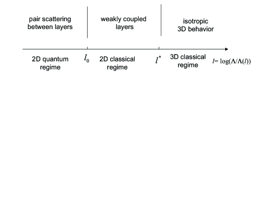
Figure 3: Regimes of the renormalization flow.

In addition to this quantum to classical crossover, the system undergoes a dimensional crossover at a scale $l^{\ast}$ defined via

$$t_{1,2}\left(l^{\ast}\right)=t_{\parallel},$$ (40)

depending whether $t_{1}\left(l^{\ast}\right)$ or $t_{2}\left(l^{\ast}\right)$ first reaches $t_{\parallel}$. In analogy to the quantum to classical crossover, it holds that excitations with momentum larger than $\Lambda e^{-l^{\ast}}$ behave quasi two dimensional while those with momentum below $\Lambda e^{-l^{\ast}}$ are sensitive to a coherent inter-layer coupling. We show that $l_{0}<l^{\ast}$ if the system is close to the critical temperature, i.e. the dimensional crossover is driven by the existence of thermal excitations in the system. However, quantum fluctuations are nevertheless crucial for the dimensional crossover, as they lead to non-local interactions $v_{ijkl}$ that are responsible for the dimensional crossover once thermally excited bosons exist.

As long as the system is in the regime $l<l^{\ast}$, the renormalized coherent inter-layer coupling is small. This has important implications for the distinction between low and high energy degrees of freedom. For $l<l^{\ast}$ we have to integrate out states with $\Lambda e^{-l}<\left|\mathbf{q}_{\parallel}\right|<\Lambda$, regardless of the momentum perpendicular to $\mathbf{q}_{\parallel}$. Only once the RG flow enters a three dimensional regime for $l>l^{\ast}$ is it sensible to distinguish low and high energy modes with momentum $q_{z}$ perpendicular to the planes. Then we integrate out states with $\Lambda e^{-l}<\sqrt{\mathbf{q}_{\parallel}^{2}+q_{z}^{2}}<\Lambda$.

We first give the one loop renormalization group equations for $l<l^{\ast}$ . It holds

$$\frac{d\mu}{dl} = 2\mu-2\sum_{lm}v_{ilmi}\int_{k}^{>}G_{lm}\left(q\right),$$

$$\frac{dt_{\perp}}{dl} = 0,$$

$$\frac{dt_{j}}{dl} = 2t_{j}+2\sum_{lm}v_{i,l,m,i+j}\int_{k}^{>}G_{lm}\left(q\right),$$

$$\frac{dT}{dl} = 2T,$$ (41)

as well as

$$\frac{dv_{ijlm}}{dl} = -\sum_{stuv}v_{ijuv}v_{stlm}\int_{q}^{>}G_{su}\left(q\right)G_{tv}\left(-q\right)$$ (42)

$$-4\sum_{stuv}v_{islu}v_{jtmv}\int_{q}^{>}G_{sv}\left(q\right)G_{tu}\left(q\right),$$

where we use the short hand notation:

$$\int_{q}^{>}...=\lim_{l\rightarrow 0}l^{-1}T\sum_{n}\int_{\Lambda e^{-l}<\left|\mathbf{q}_{\parallel}\right|<\Lambda}d^{2}q_{\parallel}...\,.$$ (43)

For $l>l^{\ast}$ the renormalized inter-layer hopping element is comparable to the in-plane hopping $t_{\parallel}$ and we are finally allowed to perform a continuum’s theory for the direction perpendicular to the layers as well. Then, the problem is identical to the one of an isotropic three dimensional Bose system

$$S = \int_{Q}^{\Lambda}\left(-i\omega_{n}+\frac{t_{\parallel}}{2}\left(q_{\parallel}^{2}+q_{z}^{2}\right)-\mu\left(l^{\ast}\right)\right)a_{Q}^{\dagger}a_{Q}$$ (44)

$$+\frac{1}{2}\int_{Q_{1}...Q_{4}}^{\Lambda}v_{iso}\left(l^{\ast}\right)a_{Q_{1}}^{\dagger}a_{Q_{2}}^{\dagger}a_{Q_{3}}a_{Q_{1}+Q_{2}-Q_{3}}\ ,$$

where $Q=(\mathbf{q}_{\parallel},q_{z},\omega_{n})$ is a $(3+1)$ -dimensional vector that includes the momentum $q_{z}$. The initial values for this flow are determined by the final values for the flow for $l<l^{\ast}$. The isotropic boson interaction

$$v_{iso}\left(l^{\ast}\right)=c\sum_{ijkl}v_{ijkl}\left(l^{\ast}\right),$$ (45)

corresponds to the $q_{z}=0$ value of the coupling constants $v_{ijkl}$. For short ranged couplings $v_{iso}$ it is dominated by the largest coupling constant. The additional prefactor $c$, with lattice constant in the $z$ -direction, ensures that $v_{iso}$ is a three dimensional coupling constant with dimension $\left[\mathrm{length}\right]^{d}\left[\mathrm{energy}\right]$ for $d=3$.

IV.1 Quantum-Classical Crossover

We first analyze the quantum to classical crossover at $l=l_{0}$. It is useful to consider separately the behavior in the quantum regime, where the renormalized temperature is small compared to the upper energy cut off $T\left(l\right)<t_{\parallel}$ and the classical regime, where $T\left(l\right)>t_{\parallel}$. We treat both regimes separately and  assume $T\left(l\right)\ll t_{\parallel}$ in the former and $T\left(l\right)\gg t_{\parallel}$ in the latter regime and connect the flow of the various coupling constants smoothly at $l_{0}$. This is essentially the approach taken in Ref.FisherHohenberg88 . The analysis of Ref.Millis93 demonstrates that the approach used here is fully consistent with results obtained using a more careful analysis of the crossover behavior.

At $T=0$, the flow of the chemical potential and of the coherent inter-layer boson hopping $t_{ij}$ are unaffected by the interaction between bosons. This result is specific for the problem of dilute bosons with $\mu<0$ since for $T=0$

$$\int_{q}^{>}G_{lm}\left(q\right)=0,$$ (46)

as a result of the integration over frequency. Physically this is due to the fact that the boson number vanishes for $T=0$ and $\mu<0$. This yields the renormalization group equations:

$$\frac{d\mu(l)}{dl} = 2\mu(l),$$

$$\frac{dt_{1,2}\left(l\right)}{dl} = 2t_{1,2}\left(l\right).$$ (47)

At $T=0$, interaction do not affect $\mu$, $t_{1}$ and $t_{2}$. This only happens once the system reaches the classical regime $l>l_{0}$. Since $t_{1,2}\left(0\right)=0$, it follows that $t_{1,2}\left(l\right)=0$ as long as the system is in the quantum regime. Quantum fluctuations do not induce a coherent hopping between layers. The inter-layer hopping $t_{ij}\left(\mathbf{k}_{\parallel}\right)=\eta_{ij}t_{\perp}k_{x}k_{y}$ remains unchanged. Note, that the amplitude $t_{\perp}$ of this inter-layer coupling is unchanged under renormalization. The flow of the chemical potential is

$$\mu\left(l\right)=\mu e^{2l}.$$ (48)

Next we analyze the behavior of the interactions.  At $T=0$ holds

$$\int_{q}^{>}G_{sv}\left(q\right)G_{tu}\left(q\right)=0,$$ (49)

which vanishes again because of the vanishing Boson density. We are left with the analysis of

$$\frac{dv_{ijlm}}{dl}=-\sum_{stuv}v_{ijuv}v_{stlm}\int_{q}^{>}G_{su}\left(q\right)G_{tv}\left(-q\right).$$ (50)

In Appendix A we analyze this flow equation in the limit where the bare inter-layer hopping $t_{\perp}$ is much smaller than the in-plane hopping $t_{\parallel}$. Up to order $\left(t_{\perp}/t_{\parallel}\right)^{4}$ we have to analyze the coupling for bosons in the same layer $v_{0}=v_{iiii}$ , in neighboring layers $v_{1}=v_{iijj}$ with $j=i\pm 1$ and second neighbor layers $v_{1}=v_{iijj}$ with $j=i\pm 2$.  We obtain at large $l$ ($l\gg 2\pi t_{\parallel}/u$):

$$v_{0}\left(l\right) \simeq \frac{2\pi t_{\parallel}a^{2}}{l}\left(1-\frac{1}{2}\left(t_{\perp}/t_{\parallel}\right)^{2}+\frac{3}{32}\left(t_{\perp}/t_{\parallel}\right)^{4}\right),$$

$$v_{1}\left(l\right) \simeq -\frac{\pi t_{\parallel}a^{2}}{2l}\left(\left(t_{\perp}/t_{\parallel}\right)^{2}-\left(t_{\perp}/t_{\parallel}\right)^{4}\right),$$

$$v_{2}\left(l\right) \simeq -\frac{\pi t_{\parallel}a^{2}}{l}\ \frac{5}{32}\left(t_{\perp}/t_{\parallel}\right)^{4}.$$ (51)

It is important to keep in mind that these results were obtained with the assumption that initially $v_{0}\left(l=0\right)=u$ is the  only coupling constant. The inter-layer interactions $v_{1}$ and $v_{2}$ result from multiple scatterings in distinct layers where virtual bosons propagate between layers. Thus, we find that there is no coherent coupling between layers in the quantum regime i.e $t_{1,2}\left(0\right)=0$. On the other hand, we do find that non-local interactions, that couple different layers, emerge. This is fully consistent with the finding of Refs.Maltsevera05; Yildirim96 .

At finite $T$, the flow in the quantum regime stops at

$$l_{0}=\frac{1}{2}\log\left(t_{\parallel}/T\right).$$ (52)

For $l>l_{0}$ thermal, as opposed to quantum fluctuations, come into play. The initial values for the subsequent flow are of course the final values of the RG flow of the quantum regime: $\mu\left(l_{0}\right)=\mu e^{2l_{0}}=t_{\parallel}\frac{\mu}{T}$ and $v_{i}\left(l_{0}\right)$ where the $v_{i}\left(l\right)$ are given in Eq.(51).

IV.2 Dimensional Crossover

The RG flows for $l>l_{0}$ continues to be two dimensional, as no coherent inter-layer was generated in the quantum regime. As discussed above we will now analyze the flow equations as if the problem was purely classical, i.e. we include solely the lowest Matsubara frequency in the evaluation of the Feynman diagrams. In this case temperature only enters the flow equations in the combination

$$w_{i}\left(l\right)=\frac{T\left(l\right)}{t_{\parallel}}v_{i}\left(l\right).$$ (53)

Thus, it is convenient to use $w_{i}\left(l\right)$ in what follows. The leading order flow equations of $w_{i}\left(l\right)$ are

$$\frac{dw_{i}\left(l\right)}{dl}=2w_{i}\left(l\right),$$ (54)

with solution

$$w_{i}\left(l\right)=w_{i}\left(l_{0}\right)e^{2\left(l-l_{0}\right)}=v_{i}\left(l_{0}\right)e^{2\left(l-l_{0}\right)}.$$ (55)

The coupling constants $w_{i}\left(l\right)$ are relevant. This is a consequence of the fact that the upper critical dimension of the classical regime is $d_{u,class.}=4$ as opposed to $d_{u,qu.}=2$ for the zero temperature quantum regime. If we wanted to determine the critical exponents of the classical phase transition, we would have to include higher order terms. As pointed out by MillisMillis93 , it is not necessary to include these higher order terms if one only wants to determine the value of the transition temperature: At low $T$, the coupling constants $v_{i}\left(l\right)$ decrease for large $l_{0}$ as follows from Eq.(51). Thus, the initial values $w_{i}\left(l_{0}\right)$ of the classical flow are small. While the interactions become relevant for $l>l_{0}$ corrections to Eq.(54) remain negligible unless the flow enters the actual critical regime. However, in our case the flow only enters the critical regime after the dimensional crossover. Thus, we can, for the moment, safely neglect corrections beyond Eq.(54).

As shown in Appendix B, the RG flow equations for the coherent hopping elements and the chemical potential in the classical regime are

$$\frac{d\mu}{dl} = 2\mu-\frac{2}{\pi}w_{0},$$

$$\frac{dt_{1}}{dl} = 2t_{1}\ ,$$

$$\frac{dt_{2}}{dl} = 2t_{2}+\frac{t_{\perp}^{2}}{\pi t_{\parallel}^{2}}\ w_{2}.$$ (56)

It immediately follows that $t_{1}\left(l\right)=0$ since $t_{1}\left(l_{0}\right)=0$. No coherent nearest neighbor hopping $t_{1}$ is being generated by the mechanism we describe. This is a consequence of the discussed $Z_{2}$-symmetry. A finite value for $t_{1}$ corresponds to a broken $Z_{2}$ symmetry.  However, the second neighbor coupling $t_{2}$ flows to a finite value even if its initial value vanishes. If we use $w_{i}\left(l\right)$ of Eq.(55) with initial values $v_{i}\left(l_{0}\right)$ from Eq.(51) it follows

$$\frac{d\mu}{dl} = 2\mu-\frac{g_{0}t_{\parallel}\ }{l_{0}}\ e^{2\left(l-l_{0}\right)},$$

$$\frac{dt_{2}}{dl} = 2t_{2}-\frac{g_{2}t_{\parallel}}{l_{0}}\ e^{2\left(l-l_{0}\right)},$$ (57)

where

$$g_{0} = 4\left(1-\frac{1}{2}\left(t_{\perp}/t_{\parallel}\right)^{2}+\frac{3}{32}\left(t_{\perp}/t_{\parallel}\right)^{4}\right),$$

$$g_{2} = \frac{5}{32}\left(t_{\perp}/t_{\parallel}\right)^{6}.$$ (58)

The solutions of these differential equations are

$$\mu\left(l\right) = e^{2\left(l-l_{0}\right)}\left(\mu\left(l_{0}\right)-\frac{g_{0}t_{\parallel}\ }{l_{0}}\left(l-l_{0}\right)\right),$$

$$t_{2}\left(l\right) = -e^{2\left(l-l_{0}\right)}\frac{g_{2}t_{\parallel}\left(l-l_{0}\right)}{l_{0}}.$$ (59)

In the last equation we already took into account that the initial value of the coherent hopping vanishes: $t_{2}\left(l_{0}\right)=0$. The dimensional crossover takes place at $l^{\ast}$ where $\left|t_{2}\left(l^{\ast}\right)\right|\simeq t_{\parallel}$, which corresponds to

$$e^{2\left(l^{\ast}-l_{0}\right)}\frac{g_{2}\left(l^{\ast}-l_{0}\right)}{l_{0}}=1.$$ (60)

For large $l^{\ast}-l_{0}$ this is equivalent to

$$e^{2\left(l^{\ast}-l_{0}\right)}\simeq\frac{l_{0}}{g_{2}\log l_{0}/g_{2}}.$$ (61)

This yields

$$w_{0}\left(l^{\ast}\right)=v_{0}\left(l_{0}\right)e^{2\left(l^{\ast}-l_{0}\right)}=v_{0}\left(l_{0}\right)\frac{l_{0}}{g_{2}\log l_{0}/g_{2}}$$ (62)

as well as

$$\mu\left(l^{\ast}\right)=\left(\frac{l_{0}}{g_{2}\log l_{0}/g_{2}}\mu\left(l_{0}\right)-\frac{g_{0}\ }{g_{2}}t_{\parallel}\right)$$ (63)

Inserting $l_{0}=\frac{1}{2}\log\left(\varepsilon_{0}/T\right)$   and $\mu\left(l_{0}\right)$ gives

$$w_{0}\left(l^{\ast}\right)=\frac{g_{0}\pi t_{\parallel}}{2}\frac{1}{g_{2}\log\left(\frac{1}{2}\log\left(t_{\parallel}/T\right)/g_{2}\right)}$$ (64)

for the value of the coupling constant at the end of the two dimensional flow and

$$\mu\left(l^{\ast}\right)=t_{\parallel}\left(\frac{\frac{1}{2}\log\left(t_{\parallel}/T\right)}{g_{2}\log\left(\frac{1}{2}\log\left(t_{\parallel}/T\right)/g_{2}\right)}\frac{\mu}{T}-\frac{g_{0}\ }{g_{2}}\right)$$ (65)

for the corresponding chemical potential. As pointed out above, for $l>l^{\ast}$, the RG probes energies sufficiently low to be sensitive to the three dimensional character of the system. These final values of the combined quantum and classical two dimensional flow become the initial value of the three dimensional flow. Since always holds $l^{\ast}>l_{0}$, it follows that this three dimensional flow is always in the classical regime.

IV.3 Flow in the Three-Dimensional Classical Regime

The final regime of the flow is in the classical three dimensional regime. The flow equations are the usual ones for an isotropic three dimensional classical bosonic system, i.e. for an two component $\varphi^{4}$ or $XY$ model. The condition for the critical temperature is that the initial values for the flow of this three dimensional classical flow obey:

$$\mu\left(l^{\ast}\right)\simeq\ w\left(l^{\ast}\right).$$ (66)

This ensures that the flow is on the critical surface and the system is close to the critical temperature. An alternative way to interpret this condition was given in Ref.Millis93 where it was shown that Eq.(66) is equivalent to the Ginzburg criterion for the onset of critical fluctuations. Whenever a system is in the Ginzburg regime of classical critical fluctuations, it is very close to the actual critical temperature. The detailed analysis inside this regime is the usual one for a $d=3$ classical $XY$ model and does not need be reproduced here. We are more interested in the value of the transition temperature at low $T$. We use our previous results for the initial values $\mu\left(l^{\ast}\right)$ and $w\left(l^{\ast}\right)$ of the three dimensional flow to analyze the condition Eq.(66)  and obtain

$$\mu = T_{c}\frac{2g_{0}\left(\frac{\pi}{2}+\log\left(\frac{1}{2g_{2}}\log\left(t_{\parallel}/T_{c}\right)\right)\right)}{\log\left(\varepsilon_{0}/T_{c}\right)}.$$ (67)

$$\simeq 8T_{c}\frac{\log\left(\frac{16}{5\varepsilon^{6}}\log\left(t_{\parallel}/T_{c}\right)\right)}{\log\left(\varepsilon_{0}/T_{c}\right)}.$$

Solving this result for $T_{c}$ with logarithmic accuracy yields the transition temperature as function of chemical potential, as given in Eq.( 11). The phase diagram that results from our RG analysis is represented in Fig.1.

V Summary

In summary, we have shown that inter–layer frustration reduces the effective dimensionality of a BEC quantum phase transition induced by a change of the chemical potential. The BEC-QCP exhibits 2D quantum critical fluctuations that dominate over an extended region of the phase diagram. The phase boundary between the disordered and ordered phase extends to finite temperatures although the universality class of the transition changes from BEC in 2+2 dimensions at $T=0$ to 3D–XY at finite $T$. For $T>0$, there is a crossover from the 2D quantum critical to a 2D classical regime as the system approaches the phase boundary from disordered side. The dimensional crossover occurs within the classical regime as the system gets even closer to the phase boundary (see Figs.1 and 3).

The BEC ordering is accompanied by bond ordering that results from a spontaneous breaking of the $Z_{2}$–symmetry discussed in section II. Both, the BEC and the bond order parameters increase continuously from zero for $\mu\to\mu_{c}$. A finite bond–order parameter induces a finite hopping between nearest–neighbor layers that vanishes at the phase boundary together with the bond ordering.

Although according to our results the thermodynamic phase transition always belongs to the 3D–XY universality class, this transition becomes more quasi–2D like as the system approaches the 2D BEC-QCP. Besides the consequences that were already discussed in the paper, like the peculiar behavior of $T_{c}(\mu)$ given by Eq.(11), this observation has implications for the $T$–dependence of any thermodynamic quantity for $T\to T_{c}$ and $\mu\gtrsim\mu_{c}(T=0)$ given the dimensional crossover predicted by our RG calculation.

The dimensional reduction at a QCP that we discussed in this paper can be experimentally verified in real quantum magnets such as BaCuSi₂O₆ Suchitra06 ; Batista07 . For quantum magnets, the chemical potential corresponds to a magnetic field applied along the symmetry axis while the particle density corresponds ot the magnetization per site. Therefore, the quantum phase transition discussed in this paper corresponds to the suppression of magnetic XY–ordering by the application of a magentic field that saturates the moments along the Z–direction. Although we discussed the case of a BCT lattice, our result can be applied to more general layered structures with frustrated inter–layer coupling.

VI Acknowledgement

We thank A. J. Millis, N. Prokof’ev and M. Vojta for helpful discussions and to M. Vojta for pointing out Ref.Yildirim96 . LANL is supported by US DOE under Contract No. W-7405-ENG-36. Ames Laboratory, is supported by US DOE under Contract No. W-7405-Eng-82.

Appendix A Appendix

A.1 Flow in the $2D$-quantum regime

In this appendix we derive the result, Eq.(51) for the interactions $v_{i}$ in the regime $l<l_{0}$ prior to the quantum to classical crossover, by solving flow equations

$$\frac{dv_{ijlm}}{dl}=-\sum_{stuv}v_{ijuv}v_{stlm}\int_{k}^{>}G_{su}\left(k\right)G_{tv}\left(-k\right).$$ (68)

We derive these results by expanding with respect to the ratio $t_{\perp}/t_{\parallel}$  of the hopping elements perpendicular and parallel to the layers. Thus we expanded  the propagator $G_{ij}\left(k\right)$ of Eq.(36) in powers of the inter-layer hopping, see Eq.(16 ). In perturbation theory in $t_{\perp}$, it always holds that $i=j$, $l=m$ , $u=v$ , and $s=t$. Thus we obtain (to simplify the notation we use $v_{ij}=v_{iijj}$):

$$\frac{dv_{ij}}{dl}=-\sum_{st}v_{it}v_{sj}\int_{q}^{>}G_{st}\left(q\right)G_{st}\left(-q\right).$$ (69)

Including terms up to order $t_{\perp}^{4}$ it follows:

$$\frac{dv_{ij}}{dl} = -\sum_{s}v_{is}v_{sj}\left(A^{\left(0\right)}+4B^{\left(2\right)}\right)\ -\sum_{st}v_{it}v_{sj}\eta_{st}A^{\left(2\right)}$$ (70)

$$-\sum_{st}v_{it}v_{sj}\sum_{l}\eta_{sl}\eta_{lt}A^{\left(4\right)},$$

where

$$A^{\left(n\right)} = \frac{t_{\perp}^{n}}{l}\int_{q}^{>}\gamma\left(q\right)^{n}g\left(q\right)^{\frac{n+2}{2}}\ g\left(-q\right)^{\frac{n+2}{2}},$$

$$B^{\left(2\right)} = \frac{t_{\perp}^{2}}{l}\int_{q}^{>}\gamma\left(q\right)^{2}g\left(q\right)\ g\left(-q\right)^{3},$$

with $\gamma\left(k\right)=k_{x}k_{y}$ and $g\left(q\right)$ of Eq.(17). Performing the frequency and momentum sums yields $A^{\left(0\right)}=(2\pi t_{\parallel})^{-1}$, $A^{\left(2\right)}=\frac{t_{\perp}^{2}}{t_{\parallel}^{2}}\left(8\pi t_{\parallel}\right)^{-1}$, $B^{\left(2\right)}=A^{\left(2\right)}/2$ as well as $A^{\left(4\right)}=t_{\perp}^{4}/t_{\parallel}^{4}\times 9\left(128\pi t_{\parallel}\right)^{-1}$. Only terms with $j=i\pm 1$ and $j=i\pm 2$ are being generated at fourth order in $t_{\perp}$. We will then introduce three different coupling constants, $v_{0}=v_{ii}$, $v_{1}=v_{i,i\pm 1}$ and $v_{2}=v_{i,i\pm 2}$. It will turn out to be crucial to include $v_{2}$ in addition to the leading non-local coupling $v_{1}$. Performing the lattice sums yields explicit flow equations for the three coupling constants. If we now keep in mind that due to the initial conditions $v_{1}\left(l=0\right)=v_{2}\left(l=0\right)=0$ vertices with $v_{1}$ are at least of order $t_{\perp}^{2}$ and vertices with $v_{2}$ are at least of order $t_{\perp}^{4}$    we can restrict the flow equations to  fourth order in $t_{\perp}$:

$$\frac{dv_{0}}{dl} = -v_{0}^{2}\widetilde{A}^{\left(0\right)}\ -2v_{1}^{2}A^{\left(0\right)}-4v_{0}v_{1}A^{\left(2\right)},$$ (71)

$$\frac{dv_{1}}{dl} = -2v_{0}v_{1}\left(A^{\left(0\right)}+4B^{\left(2\right)}\right)\ -v_{0}^{2}A^{\left(2\right)},$$

$$\frac{dv_{2}}{dl} = -\left(2v_{0}v_{2}+v_{1}^{2}\right)A^{\left(0\right)}\ -2v_{0}v_{1}A^{\left(2\right)}-v_{0}^{2}A^{\left(4\right)},$$

with $\widetilde{A}^{\left(0\right)}=A^{\left(0\right)}+4B^{\left(2\right)}+2A^{\left(4\right)}$. For large $l$ we expect a decay of the coupling constants according to $v_{\alpha}\left(l\right)\ \propto l^{-1}$ . Thus we assume

$$v_{\alpha}\left(l\right)=\frac{h_{\alpha}\left(l\right)}{l},$$ (72)

and analyze the flow equations for $h_{\alpha}\left(l\right)$. For large enough $l$ we can determine the amplitudes of the coupling constants from $\frac{dh_{\alpha}}{dl}=0$, leading to the algebraic equations

$$h_{0}\ = h_{0}^{2}\widetilde{A}^{\left(0\right)}\ +2h_{1}^{2}A^{\left(0\right)}+4h_{0}h_{1}A^{\left(2\right)},$$ (73)

$$h_{1} = 2h_{0}h_{1}\left(A^{\left(0\right)}+4B^{\left(2\right)}\right)\ +h_{0}^{2}A^{\left(2\right)},$$

$$h_{2} = \left(2h_{0}h_{2}+h_{1}^{2}\right)A^{\left(0\right)}\ +2h_{0}h_{1}A^{\left(2\right)}+h_{0}^{2}A^{\left(4\right)}.$$

We can solve this system of equations once again by expanding with respect to the small parameter

$$\alpha=A^{\left(2\right)}/A^{\left(0\right)}=\frac{1}{4}\left(t_{\perp}/t_{\parallel}\right)^{2},$$ (74)

keeping in mind that $A^{\left(4\right)}/A^{\left(0\right)}=\frac{9}{4}\alpha^{2}$. It follows

$$h_{0} = 2\pi t_{\parallel}a^{2}\left(1-2\alpha+\ \frac{7}{4}\alpha^{2}\right),$$

$$h_{1} = -2\pi t_{\parallel}a^{2}\left(\alpha-4\alpha^{2}\right),$$

$$h_{2} = -2\pi t_{\parallel}a^{2}\frac{5}{4}\alpha^{2}.$$ (75)

Inserting these results into Eq.(72) yields the result Eq.(51 ).

A.2 Flow equations in the $2D$-classical regime

As discussed in the main text, in the two dimensional classical regime we concentrate of the flow equations of the chemical potential and coherent hopping elements. We start from the general RG equations given in Eq.(41). Using the fact that $v_{ijkl}$ has only three nonvanishing contributions $v_{m}=v_{iijj}$  with $j=i\pm m$ and $m=0$ (same layer), $m=1$, neighboring layers and $m=2$ (second neighbor layers). Inserting this result into Eq.(41) yields:

$$\frac{d\mu}{dl} = 2\mu-2v_{0}\int_{k}^{>}G_{ii}\left(k\right),$$

$$\frac{dt_{1}}{dl} = 2t_{1}+2v_{1}\int_{k}^{>}G_{ii+1}\left(k\right),$$

$$\frac{dt_{2}}{dl} = 2t_{2}+2v_{2}\int_{k}^{>}G_{ii+2}\left(k\right).$$ (76)

It holds up to second order in $t_{\perp}$:

$$G_{ii}\left(k\right) \simeq g\left(k\right)+2t_{\perp}^{2}\gamma\left(k\right)^{2}g\left(k\right)^{3},$$

$$G_{ii+1}\left(k\right) \simeq t_{\perp}\gamma\left(k\right)g\left(k\right)^{2}\ ,$$

$$G_{ii+2}\left(k\right) \simeq \ t_{\perp}^{2}\gamma\left(k\right)^{2}g\left(k\right)^{3}.$$ (77)

Here we ignored effects due to $t_{1}$ and $t_{2}$ as those will only be of higher order in $t_{\perp}/t_{\parallel}$. This enables us to perform the shell integration

$$\int_{k}^{>}G_{ii}\left(k\right) = \frac{T\left(l\right)}{\pi a^{2}t_{\parallel}}\left(1+\frac{t_{\perp}^{2}}{t_{\parallel}^{2}}\right),\$$

$$\int_{k}^{>}G_{ii+1}\left(k\right) = 0,$$

$$\int_{k}^{>}G_{ii+2}\left(k\right) = \frac{T\left(l\right)}{2\pi a^{2}t_{\parallel}}\frac{t_{\perp}^{2}}{t_{\parallel}^{2}}\ ,$$ (78)

where we only included the zeroth’s Matsubara frequency in the classical regime. The contribution for the nearest neighbor coupling vanishes since $\int_{k}\gamma\left(k\right)=0$, an effect caused by the $Z_{2}$-symmetry of the Hamiltonian.  Inserting these results into Eq.(76) yields Eq.(56). The solution of the flow equations then yields values for the second neighbor hopping small by $\left(t_{\perp}/t_{\parallel}\right)^{6}$, justifying our assumption to neglect $t_{2}$ in the right hand side of Eq.(77). It is also important to notice that including terms with coherent neighbor hopping $t_{1}$ in Eq.(77) and self consistently solving the RG equation for $t_{1}$ still yields $t_{1}=0$ on the disordered side of the phase transition.

References

- (1) H. E. Stanley,“Introduction to Phase Transitions and Critical Phenomena,(Oxford University Press, Oxford, 1987).
- (2) C. D. Batista and Z. Nussinov, Phys. Rev. B 72, 045137 (2005).
- (3) C. D. Batista and G. Ortiz, Adv. in Phys. 53, 1 (2004).
- (4) Z. Nussinov and E. Fradkin, Phys. Rev. B 71, 195120 (2005).
- (5) O. Stockert et al, Phys. Rev. Lett. 80 , 5627 (1998); N. D. Mathur et al, Nature (London) 394, 39 (1998).
- (6) M. Maltseva and P. Coleman, Phys. Rev. B 72, 174415 (2005).
- (7) T. Yildirim, A. B. Harris, and E. F. Shender, Phys. Rev. B 53, 6455 (1996).
- (8) E. Shender, Sov. Phys. JETP 56, 178 (1982); C. L. Henley, Phys. Rev. Lett. 62, 2056 (1989).
- (9) C. D. Batista and S. A. Trugman, Phys. Rev. Lett. 93, 217202 (2004).
- (10) C. D. Batista, J. Schmalian, N. Kawashima, P. Sengupta, S. Sebastian, N. Harrison, M. Jaime and I. Fisher, Phys. Rev. Lett. 98, 257201 (2007).
- (11) T. Matsubara and H. Matsuda, Prog. Theor. Phys. 16, 569 (1956).
- (12) S. E. Sebastian et al, Nature 411, 617 (2006).
- (13) K. M. Sparta and G. Roth, Act. Crys. B. 60, 491 (2004).
- (14) E. Samulon et al., Phys. Rev. B 73, 100407(R) (2006).
- (15) T. Giamarchi and A. M. Tsvelik, Phys. Rev. B 59, 11398 (1999).
- (16) M. Jaime et al, Phys. Rev. Lett. 93, 087203 (2004).
- (17) O. Rösch, and M. Vojta, preprint, cond-mat/0702157.
- (18) O. Rösch, and M. Vojta, preprint, cond-mat/0705.1351.
- (19) S. E. Sebastian et al, Phys. Rev. B 74 , 180401(R) (2006).
- (20) D. S. Fisher and P. C. Hohenberg, Phys. Rev. B 37, 4936 (1988).
- (21) S. Sachdev, T. Senthil, and R. Shankar, Phys. Rev. B 50, 258 (1994).
- (22) A. J. Millis, Phys. Rev. B 48, 7183 - 7196 (1993).
- (23) For a discussion of this issue see: S. Sachdev, Quantum Phase Transitions (Cambridge Univ. Press 1999).
- (24) M. Schick, Phys. Rev. A 3, 1067 (1971).
- (25) V. N. Popov, Functional Integrals in Quantum Field Theory and Statistical Physics, Part II (Pergamon, Oxford, 1980).
- (26) S. T. Beliaev, Sov. Phys. JETP 34, 299 (1958).