Cognitive Medium Access: Exploration, Exploitation and Competition

Abstract

This paper establishes the equivalence between cognitive medium access and the competitive multi-armed bandit problem. First, the scenario in which a single cognitive user wishes to opportunistically exploit the availability of empty frequency bands in the spectrum with multiple bands is considered. In this scenario, the availability probability of each channel is unknown to the cognitive user a priori. Hence efficient medium access strategies must strike a balance between exploring the availability of other free channels and exploiting the opportunities identified thus far. By adopting a Bayesian approach for this classical bandit problem, the optimal medium access strategy is derived and its underlying recursive structure is illustrated via examples. To avoid the prohibitive computational complexity of the optimal strategy, a low complexity asymptotically optimal strategy is developed. The proposed strategy does not require any prior statistical knowledge about the traffic pattern on the different channels. Next, the multi-cognitive user scenario is considered and low complexity medium access protocols, which strike the optimal balance between exploration and exploitation in such competitive environments, are developed. Finally, this formalism is extended to the case in which each cognitive user is capable of sensing and using multiple channels simultaneously.

I Introduction

Recently, the opportunistic spectrum access problem has been the focus of significant research activity [1, 2, 3]. The underlying idea is to allow unlicensed users (i.e., cognitive users) to access the available spectrum when the licensed users (i.e., primary users) are not active. The presence of high priority primary users and the requirement that the cognitive users should not interfere with them define a new medium access paradigm which we refer to as cognitive medium access. The overarching goal of our work is to develop a unified framework for the design of efficient, and low complexity, cognitive medium access protocols.

The spectral opportunities available to the cognitive users are expected to be time-varying on different time-scales. For example, on a small scale, multimedia data traffic of the primary users will tend to be bursty [4]. On a large scale, one would expect the activities of each user to vary throughout the day. Therefore, to avoid interfering with the primary network, the cognitive users must first probe to determine whether there are primary activities in each channel before transmission. Under the assumption that each cognitive user cannot access all of the available channels simultaneously, the main task of the medium access protocol is to distributively choose which channels each cognitive user should attempt to use in different time slots, in order to fully (or maximally) utilize the spectral opportunities. This decision process can be enhanced by taking into account any available statistical information about the primary traffic. For example, with a single cognitive user capable of accessing (sensing) only one channel at a time, the problem becomes trivial if the probability that each channel is free is known a priori. In this case, the optimal rule is for the cognitive user to access the channel with the highest probability of being free in all time slots. However, such time-varying traffic information is typically not available to the cognitive users a priori. The need to learn this information on-line creates a fundamental tradeoff between exploitation and exploration. Exploitation refers to the short-term gain resulting from accessing the channel with the estimated highest probability of being free (based on the results of previous sensing decisions) whereas exploration is the process by which the cognitive user learns the statistical behavior of the primary traffic (by choosing possibly different channels to probe across time slots). In the presence of multiple cognitive users, the medium access algorithm must also account for the competition between different users over the same channel.

In this paper, we develop a unified framework for the design and analysis of cognitive medium access protocols. As argued in the sequel, this framework allows for the construction of strategies that strike an optimal balance among exploration, exploitation and competition. The key observation motivating our approach is the equivalence between our problem and the classical multi-armed bandit problem (see [5] and references therein). This equivalence allows for building a solid foundation for cognitive medium access using tools from reinforcement machine learning [6]. The connection between cognitive medium access and the multi-armed bandit problem has been independently and concurrently observed in [7]. That work, however, is limited to special cases of the general approach presented here. In particular, in [7], the channels are assumed to be independent and the goal is to maximize the discounted sum of throughput, which is the problem addressed in Example 4 in Section III below. A related work also appears in [8], in which the availability of each channel is assumed to follow a Markov chain, whose transition matrix is known to the cognitive user. The only uncertainty faced by the cognitive user in that work is the particular realization of the channel, while in our work the cognitive users also need to learn the statistics of the channel in real time.

We consider three scenarios in this paper. In the first scenario, we assume the existence of a single cognitive user capable of accessing only a single channel at any given time. In this setting, we derive an optimal sensing rule that maximizes the expected throughput obtained by the cognitive user. Compared with a genie-aided scheme, in which the cognitive user knows a priori the primary network traffic information, there is a throughput loss suffered by any medium access strategy. We obtain a lower bound on this loss and further construct a linear complexity single index protocol that achieves this lower bound asymptotically (when the primary traffic behavior changes very slowly). In the second scenario, we design distributed sensing rules that account for the competitive dimension of the problem in which the cognitive users must also take the competition from other cognitive users into consideration when making sensing decisions. We first characterize the optimal distributed sensing rule for the case in which the traffic information of the primary network is available to the cognitive users. Under this idealistic assumption, we show that the throughput loss of the proposed distributed sensing rule, compared with a throughput optimal centralized scheme, goes to zero exponentially as the number of cognitive users increases. To prevent any possible misbehavior by the cognitive users, we further design a game theoretically fair sensing rule, whose loss compared with the throughput optimal centralized rule also goes to zero exponentially. Building on these results, we then devise distributed sensing rules that do not require prior knowledge about the traffic and converge to the optimal distributed rule and game theoretically fair rule, respectively. In the third scenario, we extend our work to the case in which the cognitive user is capable of accessing more than one channel simultaneously.

The rest of the paper is organized as follows. Our network model is detailed in Section II. Section III analyzes the scenario in which a single cognitive user capable of sensing one channel at a time is present. The extension to the multi-user case is reported in Section IV whereas the multi-channel extension is studied in Section V. Finally, Section VI summarizes our conclusions.

II Network Model

Throughout this paper, upper-case letters (e.g., $X$) denote random variables, lower-case letters (e.g., $x$) denote realizations of the corresponding random variables, and calligraphic letters (e.g, $\mathcal{X}$) denote finite alphabet sets over which corresponding variables range. Also, upper-case boldface letters (e.g., $\mathbf{X}$) denote random vectors and lower-case boldface letters (e.g., $\mathbf{x}$) denote realizations of the corresponding random vectors.

Figure 1 shows the channel model of interest. We consider a primary network consisting of $N$ channels, $\mathcal{N}=\{1,\cdots,N\}$, each with bandwidth $B$. The users in the primary network are operated in a synchronous time-slotted fashion. We use $i$ to refer to the channel index, $j$ to refer to the time-slot index and $k$ referring to the index of the cognitive users. We assume that at each time slot, channel $i$ is free with probability $\theta_{i}$. Let $Z_{i}(j)$ be a random variable that equals $1$ if channel $i$ is free at time slot $j$ and equals $0$ otherwise. Hence, given $\theta_{i}$, $Z_{i}(j)$ is a Bernoulli random variable with probability density function (pdf)

$$h_{\theta_{i}}(z_{i}(j))=\theta_{i}\delta(1)+(1-\theta_{i})\delta(0),$$

where $\delta(\cdot)$ is the delta function. Furthermore, for a given $\hbox{\boldmath$\theta$}=(\theta_{1},\cdots,\theta_{N})$, $Z_{i}(j)$ are independent for each $i$ and $j$. We consider a block varying model in which the value of $\theta$ is fixed for a block of $T$ time slots and randomly changes at the beginning of the next block according to some joint pdf $f(\hbox{\boldmath$\theta$})$. Our results can also be extended to the scenarios in which $Z_{i}(j)$s follow a Markov chain model.

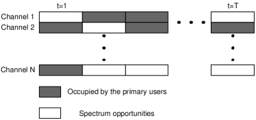
Figure 1: Channel model.

In our model, the cognitive users attempt to exploit the availability of free channels in the primary network by sensing the activity at the beginning of each time slot. Our work seeks to characterize efficient strategies for choosing which channels to sense (access). The challenge here stems from the fact that the cognitive users are assumed to be unaware of $\theta$ a priori. We consider two cases in which the cognitive user either has or does not have prior information about the pdf of $\theta$, i.e., $f(\hbox{\boldmath$\theta$})$. To further illustrate the point, let us consider our first scenario in which a single cognitive user capable of sensing only one channel is present. At time slot $j$, the cognitive user selects one channel $S(j)\in\mathcal{N}$ to access. If the sensing result shows that channel $S(j)$ is free, i.e., $Z_{S(j)}(j)=1$, the cognitive user can send $B$ bits over this channel; otherwise, the cognitive user will wait until the next time slot and pick a possibly different channel to access (throughout the paper, it is assumed that the outcome of the sensing algorithm is error free). Therefore, the total number of bits that the cognitive user is able to send over one block (of $T$ time slots) is

$$W=\sum\limits_{j=1}^{T}BZ_{S(j)}(j).$$

It is now clear that $W$ is a random variable that depends on the traffic in the primary network and, more importantly for us, on the medium access protocols employed by the cognitive user. Therefore, the overarching goal of Section III is to construct low complexity medium access protocols that maximize

$$\mathbb{E}\{W\}=\mathbb{E}\left\{\sum\limits_{j=1}^{T}BZ_{S(j)}(j)\right\}.$$ (1)

Intuitively, the cognitive user would like to select that channel with the highest probability of being free in order to obtain more transmission opportunities. If $\theta$ is known then this problem is trivial: the cognitive user should choose the channel $i^{*}=\arg\max\limits_{i\in\mathcal{N}}\theta_{i}$ to sense. The uncertainty in $\theta$ imposes a fundamental tradeoff between exploration, in order to learn $\theta$, and exploitation, by accessing the channel with the highest estimated free probability based on current available information, as detailed in the following sections.

III Single User–Single Channel

We start by developing the optimal solution to the single user–single channel scenario under the idealized assumption that $f(\hbox{\boldmath$\theta$})$ is known a priori by the cognitive user. As argued next, the optimal medium access algorithm suffers from a prohibitive computational complexity that grows exponentially with the block length $T$. This motivates the design of low complexity asymptotically optimal approaches that are considered next. Interestingly, the proposed low complexity technique does not require prior knowledge about $f(\hbox{\boldmath$\theta$})$.

III-A Bayesian Approach

Our single user–single channel cognitive medium access problem belongs to the class of bandit problems. In this setting, the decision maker must sequentially choose one process to observe from $N\geq 2$ stochastic processes. These processes usually have parameters that are unknown to the decision maker and, associated with each observation is a utility function. The objective of the decision maker is to maximize the sum or discounted sum of the utilities via a strategy that specifies which process to observe for every possible history of selections and observations. The following classical example illustrates the challenge facing our decision maker: A gambler enters a casino having $N$ slot machines, the $i^{th}$ of which has winning probability $\theta_{i},i\in\mathcal{N}$. The gambler does not know the values of the $\theta_{i}$s and must sequentially chooses machines to play. The goal is to maximize the overall gain for a total of $T$ plays. In this example, the stochastic processes are the outcomes of the slot machines, the utility function is the reward that the gambler gains each time and the gambling strategy specifies which machine to play based on each possible past information pattern. A comprehensive treatment covering different variants of bandit problems can be found in [5].

We are now ready to rigorously formulate our problem. The cognitive user employs a medium access strategy $\Gamma$, which will select channel $S(j)\in\mathcal{N}$ to sense at time slot $j$ for any possible causal information pattern obtained through the previous $j-1$ observations:

$$\Psi(j)=\{s(1),z_{s(1)}(1),\cdots,s(j-1),z_{s(j-1)}(j-1)\},j\geq 2,$$

i.e. $s(j)=\Gamma(f,\Psi(j))$. Notice that $z_{s(j)}(j)$ is the sensing outcome of the $j$th time slot, in which $s(j)$ is the channel being accessed. If $j=1$, there is no accumulated information, thus $\Psi(1)=\phi$ and $s(1)=\Gamma(f)$. $\Gamma$ could be stochastic, i.e., for certain $\Psi(j)$, the cognitive user may randomly pick channel $i$ from a set $\mathcal{A}\subseteq\mathcal{N}$ with probability $p_{i}$, such that $\sum\limits_{i\in\mathcal{A}}p_{i}=1$. The utility that the cognitive user obtains by making decision $S(j)$ at time slot $j$ is the number of bits it can transmit at time slot $j$, which is $BZ_{S(j)}(j)$. We denote the expected value of the payoff obtained by a cognitive user who uses strategy $\Gamma$ as

$$W_{\Gamma}=\mathbb{E}_{f}\left\{\sum\limits_{j=1}^{T}BZ_{S(j)}(j)\right\}.$$ (2)

We denote $V^{*}(f,T)=\sup\limits_{\Gamma}W_{\Gamma}$, which is the largest throughput that the cognitive user could obtain when the spectral opportunities are governed by $f(\hbox{\boldmath$\theta$})$ and the exact value of each realization of $\theta$ is not known by the user.

Each medium access decision made by the cognitive user has two effects. The first one is the short term gain, i.e., an immediate transmission opportunity if the chosen channel is found free. The second one is the long term gain, i.e., the updated statistical information about $f(\hbox{\boldmath$\theta$})$. This information will help the cognitive user in making better decisions in the future stages. There is an interesting tradeoff between the short and long term gains. If we only want to maximize the short term gain, we can pick the one with the highest free probability to sense, based on the current information. This myopic strategy maximally exploits the existing information. On the other hand, by picking other channels to sense, we gain valuable statistical information about $f(\hbox{\boldmath$\theta$})$ which can effectively guide future decisions. This process is typically referred to as exploration.

More specifically, let $f^{j}(\hbox{\boldmath$\theta$})$ be the updated pdf after making $j-1$ observations. We begin with $f^{1}(\hbox{\boldmath$\theta$})=f(\hbox{\boldmath$\theta$})$. After observing $z_{s(j)}(j)$, we update the pdf using the following Bayesian formula.

1. If $z_{s(j)}(j)=1$

   $$f^{j+1}(\hbox{\boldmath$\theta$})=\frac{\theta_{s(j)}f^{j}(\hbox{\boldmath$\theta$})}{\int\theta_{s(j)}f^{j}(\hbox{\boldmath$\theta$})d\hbox{\boldmath$\theta$}},$$ (3)

2. If $z_{s(j)}(j)=0$

   $$f^{j+1}(\hbox{\boldmath$\theta$})=\frac{\left(1-\theta_{s(j)}\right)f^{j}(\hbox{\boldmath$\theta$})}{\int\left(1-\theta_{s(j)}\right)f^{j}(\hbox{\boldmath$\theta$})d\hbox{\boldmath$\theta$}}.$$ (4)

Now, lemma 2.3.1 of [5] proves that every bandit problem with finite horizon has an optimal solution. Applying this result to our set-up, we obtain the following.

Lemma 1

For any prior pdf $f$, there exists an optimal strategy $\Gamma^{*}$ to the channel selection problem (2), and $V^{*}(f,T)$ is achievable. Moreover, $V^{*}$ satisfies the following condition:

$$V^{*}(f,T)=\max\limits_{s(1)\in\mathcal{N}}\mathbb{E}_{f}\left\{BZ_{s(1)}+V^{*}\left(f_{Z_{s(1)}},T-1\right)\right\},$$ (5)

where $f_{Z_{s(1)}}$ is the conditional pdf updated using (3) and (4) as if the cognitive user chooses $s(1)$ and observes $Z_{s(1)}$. Also, $V^{*}\left(f_{Z_{s(1)}},T-1\right)$ is the value of a bandit problem with prior information $f_{Z_{s(1)}}$ and $T-1$ sequential observations.∎

In principle, Lemma 1 provides the solution to problem (2). Effectively, it decouples the calculation at each stage, and hence, allows the use of dynamic programming to solve the problem. The idea is to solve the channel selection problem with a smaller dimension first and then use backward deduction to obtain the optimal solution for a problem with a larger dimension. Starting with $T=1$, the second term inside the expectation in (5) is 0, since $T-1=0$. Hence, the optimal solution is to choose channel $i$ with the largest $\mathbb{E}_{f}\{BZ_{i}\}$, which can be calculated as

$$\mathbb{E}_{f}\{BZ_{i}\}=B\int\theta_{i}f(\hbox{\boldmath$\theta$})d\hbox{\boldmath$\theta$}.$$

And $V^{*}(f,1)=\max\limits_{i\in\mathcal{N}}\mathbb{E}_{f}\{BZ_{i}\}$.

With the solution for $T=1$ at hand, we can now solve the $T=2$ case using (5). At first, for every possible choice of $s(1)$ and possible observation $z_{s(1)}$, we calculate the updated pdf $f_{z_{s(1)}}$ using (3) and (4). Next, we calculate $V^{*}(f_{z_{s(1)}},1)$ (which is equivalent to the $T=1$ problem described above). Finally, applying (5), we have the following equation for the channel selection problem with $T=2$

$$V^{*}(f,2) = \max\limits_{i\in\mathcal{N}}\int\left[B\theta_{i}+\theta_{i}V^{*}(f_{z_{i}=1},1)\right.$$

$$\hskip 34.1433pt\left.+(1-\theta_{i})V^{*}(f_{z_{i}=0},1)\right]f(\hbox{\boldmath$\theta$})d\hbox{\boldmath$\theta$}.$$

Correspondingly, the optimal solution is $\Gamma^{*}(f)=\arg\max\limits_{i\in\mathcal{N}}V^{*}(f,2)$, i.e., in the first step, the cognitive user should choose $i^{*}(1)=\arg\max\limits_{i\in\mathcal{N}}V^{*}(f,2)$ to sense. After observing $z_{i^{*}(1)}$, the cognitive user has $\Psi(1)=\{z_{i^{*}(1)}\}$, and it should choose $i^{*}(2)=\arg\max\limits_{i\in\mathcal{N}}V^{*}(f_{z_{i^{*}(1)}},1)$ implying that $\Gamma^{*}(f,\Psi(1))=\arg\max\limits_{i\in\mathcal{N}}V^{*}(f_{z_{i^{*}(1)}},1)$.

Similarly, after solving the $T=2$ problem, one can proceed to solve the $T=3$ case. Using this procedure recursively, we can solve the problem with $T-1$ observations. Finally, our original problem with $T$ observations is solved as follows.

$$V^{*}(f,T) = \max\limits_{i\in\mathcal{N}}\int\left[B\theta_{i}+\theta_{i}V^{*}(f_{z_{i}=1},T-1)\right.$$

$$\hskip 22.76219pt\left.+(1-\theta_{i})V^{*}(f_{z_{i}=0},T-1)\right]f(\hbox{\boldmath$\theta$})d\hbox{\boldmath$\theta$}.$$

Example 1

Suppose we have two channels and two observations per block, i.e., $\mathcal{N}=\{1,2\}$ and $T=2$. The channels are known to be either both very busy or both relatively idle which is reflected in the following joint pdf

$$f(\theta_{1},\theta_{2})=\frac{4}{5}\delta(0.1,0)+\frac{1}{5}\delta(0.8,1),$$

where $\delta(x,y)$ is the delta function at point $(x,y)$. For simplicity of presentation, we assume that $B=100$.

In this example, on the average, channel $1$ is available with probability $4/5\times 0.1+1/5\times 0.8=0.24$, whereas channel $2$ is available with probability $4/5\times 0+1/5\times 1=0.2$. Hence, if the cognitive user ignores the information gained from sensing, it should always choose channel $1$ to sense, resulting in an average throughput of $2\times 0.24\times 100=48$ bits per block. Now, we use the procedure described above to derive the optimal rule and corresponding throughput.

1) First calculate all possible updated pdf after one step.

If $s(1)=1,z_{s(1)}=1$, we have

$$P(\theta_{1}=0.1,\theta_{2}=0|z_{s(1)}=1)$$

$$=\frac{P(z_{1}=1|\theta_{1}=0.1,\theta_{2}=0)P(\theta_{1}=0.1,\theta_{2}=0)}{P(z_{1}=1)}$$

$$=\frac{0.1\times 0.8}{0.8\times 0.1+0.2\times 0.8}=\frac{1}{3}.$$

Hence, for this case, we have

$$f_{\{s(1)=1,z_{s(1)}=1\}}=\frac{1}{3}\delta(0.1,0)+\frac{2}{3}\delta(0.8,1).$$

Similarly, we obtain the following updated pdf

$$f_{\{s(1)=1,z_{s(1)}=0\}} = \frac{18}{19}\delta(0.1,0)+\frac{1}{19}\delta(0.8,1),$$

$$f_{\{s(1)=2,z_{s(1)}=1\}} = \delta(0.8,1),$$

$$f_{\{s(1)=2,z_{s(1)}=0\}} = \delta(0.1,0).$$

2) With the updated distribution information, we solve four channel-selection problems with $T=1$. For example, with $f_{\{s(1)=1,z_{s(1)}=1\}}=\frac{1}{3}\delta(0.1,0)+\frac{2}{3}\delta(0.8,1)$, if the cognitive user choose channel 1, the expected payoff would be

$$100\times\left(\frac{1}{3}\times 0.1+\frac{2}{3}\times 0.8\right)=\frac{170}{3}.$$

If the cognitive user choose channel $2$, the expected payoff would be

$$100\times\left(\frac{1}{3}\times 0+\frac{2}{3}\times 1\right)=\frac{200}{3}.$$

Thus

$$V^{*}(f_{\{s(1)=1,z_{s(1)}=1\}},1)=\max\{170/3,200/3\}=200/3,$$

and the user should choose channel $2$.

Similarly, we have

$$V^{*}(f_{\{s(1)=1,z_{s(1)}=0\}},1)=100\times\max\{26/190,1/19\}=260/19,$$

and the user should choose channel $1$.

$$V^{*}(f_{\{s(1)=2,z_{s(1)}=1\}},1)=\max\{80,100\}=100,$$

and the user should choose channel $2$.

$$V^{*}(f_{\{s(1)=2,z_{s(1)}=0\}},1)=\max\{10,0\}=10,$$

and the user should choose channel $1$.

3) Finally, we solve the problem with pdf $f$ and $T=2$. If the cognitive user chooses channel $1$ in the first step, we calculate

$$\mathbb{E}_{f}\{BZ_{1}+V^{*}(f_{Z_{1}},1)\}$$

$$=P(\theta_{1}=0.1)\Big{[}100\times 0.1+0.1\times V^{*}(f_{\{s(1)=1,z_{s(1)}=1\}},1)$$

$$\hskip 28.45274pt+(1-0.1)\times V^{*}(f_{\{s(1)=1,z_{s(1)}=0\}},1)\Big{]}$$

$$+P(\theta_{1}=0.8)\Big{[}100\times 0.8+0.8\times V^{*}(f_{\{s(1)=1,z_{s(1)}=1\}},1)$$

$$\hskip 28.45274pt+(1-0.8)\times V^{*}(f_{\{s(1)=1,z_{s(1)}=0\}},1)\Big{]}$$

$$=252/5.$$

Similarly, if the cognitive user chooses channel $2$ in the first step, we calculate

$$\mathbb{E}_{f}\{BZ_{2}+V^{*}(f_{Z_{2}},1)\}$$

$$=P(\theta_{2}=0)\Big{[}100\times 0+0\times V^{*}(f_{\{s(1)=2,z_{s(1)}=1\}},1)$$

$$+V^{*}(f_{\{s(1)=2,z_{s(1)}=0\}},1)\Big{]}$$

$$+P(\theta_{2}=1)\Big{[}100+V^{*}(f_{\{s(1)=2,z_{s(1)}=1\}},1)$$

$$+(1-1)V^{*}(f_{\{s(1)=0,z_{s(1)}=0\}},1)\Big{]}$$

$$=P(\theta_{2}=0)V^{*}(f_{\{s(1)=2,z_{s(1)}=0\}},1)$$

$$+P(\theta_{2}=1)[100+V^{*}(f_{\{s(1)=2,z_{s(1)}=1\}},1)]=\frac{240}{5}.$$

Thus

$$V^{*}(f,2) = \max\limits_{s(1)\in\mathcal{N}}\mathbb{E}_{f}\left\{BZ_{s(1)}+V^{*}\left(f_{Z_{s(1)}},1\right)\right\}$$

$$=\max\{252/5,240/5\}=252/5.$$

Hence, the optimal strategy is $\Gamma^{*}(f)=1$, $\Gamma^{*}(f,z_{1}=1)=2$, $\Gamma^{*}(f,z_{1}=0)=1$. In other words, the cognitive user should sense channel $1$ in the first time slot. Interestingly, if channel $1$ is found free, the user should switch to channel $2$ in the second time slot. On the other hand, if channel $1$ is found busy, the cognitive user should keep sensing channel $1$ at the second time slot. Finally, we observe that the optimal strategy offers a gain of $12/5$ bits, on average, as compared with the myopic strategy.∎

The optimal solution presented above can be simplified when $f(\hbox{\boldmath$\theta$})$ has a certain structure, as illustrated by the following examples.

Example 2

(Symmetric Channels) We have $N=2$ channels. Without loss of generality, let $0\leq\theta_{b}<\theta_{a}\leq 1$. At any block, either 1) channel $1$ has probability $\theta_{a}$ of being free and channel $2$ has probability $\theta_{b}$ of being free or 2) channel $1$ has probability $\theta_{b}$ of being free and channel $2$ has probability $\theta_{a}$ of being free. The cognitive user does not know exactly which case happens. The prior pdf information is thus given by

$$f(\theta_{1},\theta_{2})=\xi\delta(\theta_{a},\theta_{b})+(1-\xi)\delta(\theta_{b},\theta_{a}),$$

where $\xi$ is a parameter. The optimal strategy under this scenario is the following.

1. At the first time slot, choose channel $1$, if $\xi>1/2$. If $\xi=1/2$, randomly choose channel $1$ or channel $2$. Otherwise choose channel $2$.

2. At time slots $j\geq 2$, update the pdf based on $\Psi(j)=\{s_{1},z_{s_{1}},\cdots,s_{j-1},z_{s_{j-1}}\}$ using (3) and (4). It is easy to see that $f^{j}$ has the following form

   $$f^{j}(\theta_{1},\theta_{2})=\xi_{j}\delta(\theta_{a},\theta_{b})+(1-\xi_{j})\delta(\theta_{b},\theta_{a}).$$

   Then, choose channel $1$ if $\xi_{j}>1/2$, randomly choose channel $1$ or $2$ if $\xi_{j}=1/2$ and choose channel $2$ otherwise.

The optimality of this myopic strategy was proved in [9].

The previous myopic strategy is also optimal for some other special scenarios. For example, if the prior pdf is $f(\hbox{\boldmath$\theta$})=\xi\delta(a,b)+(1-\xi)\delta(c,d)$, then any of the following conditions ensures the optimality of the myopic strategy [10]: 1) $a+b=c+d=1$, 2) $a\leq b$ and $c\leq d$, 3) $a\geq b$ and $c\geq d$. ∎

Example 3

(One Known Channel) We have $N=2$ channels with independent traffic distributions. Channel 1 and channel 2 are independent. Moreover, $\theta_{2}$ is known. The traffic pattern of channel $1$ is unknown, and the probability density function of $\theta_{1}$ is given by $f_{1}(\theta_{1})$.

Since channel $2$ is known and is independent of channel $1$, sensing channel $2$ will not provide the cognitive user with any new information. Hence, once the cognitive user starts accessing channel $2$ (meaning that at a certain stage, sensing channel $2$ is optimal), there would be no reason to return to channel $1$ in the optimal strategy. A generalized version of this assertion was first proved in Lemma 4.1 of [11]. Restated in our channel selection setup, we have the following lemma.

Lemma 2

In the optimal medium access strategy, once the cognitive user starts accessing channel $2$, it should keep picking the same channel in the remaining time slots, regardless of the outcome of the sensing process.∎

This lemma essentially converts the channel selection problem to an optimal stopping problem [12, 13], where we only need to focus on the strategies that decide at which time-slot we should stop sensing channel $1$, if it is ever accessed. The following lemma derives the optimal stopping rule.

Lemma 3

For any $f_{1}(\theta_{1})$ and any $T$, if $\theta_{2}\geq\Lambda(f_{1},T)$, then we should sense channel 2. Here

$$\Lambda(f_{1},T)=\max\limits_{\Gamma(f_{1})=1}\frac{\mathbb{E}_{f_{1}}\left\{\sum_{j=1}^{M}Z_{1}(j)\right\}}{\mathbb{E}_{f_{1}}\{M\}},$$ (6)

where $\Gamma$ are the set of strategies that start with channel $1$ and never switch back to channel $1$ after selecting channel $2$; and $M$ is a random number that represents the last time slot in which channel $1$ is sensed, when the cognitive user follows a strategy in $\Gamma$.

Proof:

This result follows as a direct application of Theorem 5.3.1 and Corollary 5.3.2 of [5]. ∎

One can now combine Lemma 2 and Lemma 3 to obtain the following optimal strategy.

1. At any time slot $j$, if channel $2$ was sensed at time slot $j-1$, keep sensing channel 2.

2. If channel $1$ was sensed at time slot $j-1$, update the pdf $f^{j}$ using (3) and (4) and compute $\Lambda(f_{1}^{j},T-j+1)$ using (6). If $\Lambda(f_{1}^{j},T-j+1)<\theta_{2}$, switch to channel $2$; otherwise, keep sensing channel $1$.∎

Example 4

(Independent Channels)

We have $N$ independent channels with $f(\hbox{\boldmath$\theta$})=\prod\limits_{i=1}^{N}f_{i}(\theta_{i})$. This case has a simple form of solution in the asymptotic scenario $T\rightarrow\infty$ assuming the following discounted form for the utility function

$$W=\mathbb{E}_{f}\left\{\sum\limits_{j=1}^{\infty}\alpha^{j}BZ_{S(j)}(j)\right\},$$

where $0<\alpha<1$ is a discount factor. As discussed in the introduction, this scenario has been considered in [7], and the optimal strategy for this scenario is the following.

1. If channel $l$ was selected at time slot $j-1$, then we get the updated pdf $f_{l}^{j}$ using equations (3) and (4), based on the sensing result $z_{l}(j-1)$. For other channels, we let $f_{i}^{j}=f_{i}^{j-1},\forall i\neq l,i\in\mathcal{N}$. That is we only update the pdf of the channel which was just accessed (due to the independence assumption).

2. For each channel, we calculate an index using the following equation

   $$\Lambda_{i}(f_{i}^{j})=\max\limits_{\Gamma(f_{i}^{j})=i}\frac{\mathbb{E}_{f_{i}^{j}}\left\{\sum_{j=1}^{M}\alpha^{j}Z_{1}(j)\right\}}{\mathbb{E}_{f_{i}^{j}}\{\sum_{j=1}^{M}\alpha^{j}\}},$$

   where $\Gamma$ is the set of strategies for the equivalent One-Known-Channel selection problem (with channel $i$ having the unknown parameter) and $M$ is a random number corresponding to the last time slot in which channel $i$ will be selected in the equivalent One-Known-Channel case. $\Lambda_{i}$ is typically referred to as the Gittins Index [14].

3. Choose the channel with the largest Gittins index to sense at time slot $j$.

The optimality of this strategy is a direct application of the elegant result of Gittins and Jones [14]. Computational methods for evaluating the Gittins Index $\Lambda$ could be found in [15] and references therein.

III-B Non-parametric Asymptotic Analysis and Asymptotically Optimal Strategies

The optimal solution developed in Section III-A suffers from a prohibitive computational complexity. In particular, the dimensionality of our search dimension grows exponentially with the block length $T$. Moreover, one can envision many practical scenarios in which it would be difficult for the cognitive user to obtain the prior information $f(\hbox{\boldmath$\theta$})$. This motivates our pursuit of low complexity non-parametric protocols which maintain certain optimality properties. Towards this end, we study in the following the asymptotic performance of several low complexity approaches. In this section, we analyze non-parametric schemes that do not explicitly use $f(\hbox{\boldmath$\theta$})$, thus the rules $\Gamma$ considered in this section depend only on $\Psi(j)$ explicitly. We aim to develop schemes that have low complexity but still maintain certain optimality. Towards this end, we study the asymptotic performance of schemes as the block length $T$ increases. This section will be concluded with our asymptotically optimal non-parametric protocols which require only linear computational complexity.

For a certain strategy $\Gamma$, the expected number of bits the cognitive user is able to transmit through a block with certain parameters $\theta$ is

$$\mathbb{E}\left\{\sum\limits_{j=1}^{T}BZ_{S(j)}(j)\right\}=\sum\limits_{j=1}^{T}B\sum\limits_{i=1}^{N}\theta_{i}\text{Pr}\left\{\Gamma(\Psi(j))=i\right\}.$$

Recall that $\Gamma(\Psi(j))=i$ means that, following strategy $\Gamma$, the cognitive user should choose channel $i$ at time slot $j$, based on the available information $\Psi(j)$. Here $\text{Pr}\left\{\Gamma(\Psi(j))=i\right\}$ is the probability that the cognitive user will choose channel $i$ at time slot $j$, following the strategy $\Gamma$.

Compared with the idealistic case where the exact value of $\theta$ is known, in which the optimal strategy for the cognitive user is to always choose the channel with the largest free probability, the loss entailed by $\Gamma$ is given by

$$L(\hbox{\boldmath$\theta$};\Gamma)=\sum\limits_{j=1}^{T}B\theta_{i^{*}}-\sum\limits_{j=1}^{T}B\sum\limits_{i=1}^{N}\theta_{i}\text{Pr}\left\{\Gamma(\Psi(j))=i\right\},$$

where $\theta_{i^{*}}=\max\{\theta_{1},\cdots,\theta_{N}\}$. We say that a strategy $\Gamma$ is consistent, if for any $\hbox{\boldmath$\theta$}\in[0,1]^{N}$, there exists $\beta<1$ such that $L(\hbox{\boldmath$\theta$};\Gamma)$ scales as $O(T^{\beta})$. For example, consider a royal scheme in which the cognitive user selects channel $i$ at the beginning of a block and sticks to it. If $\theta_{i}$ is the largest one among $\theta$, $L(\hbox{\boldmath$\theta$};\Gamma)=0$. On the other hand, if $\theta_{i}$ is not the largest one, $L(\hbox{\boldmath$\theta$};\Gamma)\sim O(T)$. Hence, this royal scheme is not consistent. The following lemma characterizes the fundamental limits of any consistent scheme.

Lemma 4

For any $\theta$ and any consistent strategy $\Gamma$, we have

$$\lim\inf\limits_{T\rightarrow\infty}\frac{L(\hbox{\boldmath$\theta$};\Gamma)}{\ln T}\geq B\sum\limits_{i\in\mathcal{N}\backslash\{i^{*}\}}\frac{\theta_{i^{*}}-\theta_{i}}{D(\theta_{i}||\theta_{i}^{*})},$$ (7)

where $D(\theta_{i}||\theta_{l})$ is the Kullback-Leibler divergence between the two Bernoulli random variables with parameters $\theta_{i}$ and $\theta_{l}$ respectively:

$$D(\theta_{i}||\theta_{l})=\theta_{i}\ln\left(\frac{\theta_{i}}{\theta_{l}}\right)+(1-\theta_{i})\ln\left(\frac{1-\theta_{i}}{1-\theta_{l}}\right).$$

Proof:

The proof is an application of a theorem proved in [16]. More specifically, for a general bandit problem, let $x$ be the random payoff obtained by choosing bandit $i$ (not necessarily Bernoulli), and we also let $h_{\theta_{i}}(x)$ be the pdf of $x$ for a given $\theta_{i}$.

Let $\mu_{i}$ denote the average payoff of bandit $i$, i.e.

$$\mu_{i}=\int xh_{\theta_{i}}(x)dx,$$

and note that the Kullback-Leibler divergence between bandit $i$ and $l$ is given by

$$D(\theta_{i}||\theta_{l})=\int\Big{[}\ln h_{\theta_{i}}(x)-\ln h_{\theta_{l}}(x)\Big{]}h_{\theta_{i}}(x)dx.$$

Let $i^{*}=\arg\max\limits_{i\in\mathcal{N}}\mu_{i}$, i.e., the index of the channel with the largest average payoff. Under mild regularity conditions on $h_{\theta_{i}}(x)$, it has been proved in Theorem 1 of [16] that for any consistent strategy $\Gamma$

$$\lim\inf\limits_{T\rightarrow\infty}\frac{L(\hbox{\boldmath$\theta$};\Gamma)}{\ln T}\geq\sum\limits_{i\in\mathcal{N}\backslash\{i^{*}\}}\frac{\mu_{i^{*}}-\mu_{i}}{D(\theta_{i}||\theta_{i}^{*})}.$$ (8)

In our cognitive radio channel selection problem, given $\theta$, $x$ is a random variable with

$$h_{\theta_{i}}(x)=\theta_{i}\delta(B)+(1-\theta_{i})\delta(0);$$

hence $\mu_{i}=B\theta_{i}$, and

$$D(\theta_{i}||\theta_{l})=\theta_{i}\ln\left(\frac{\theta_{i}}{\theta_{l}}\right)+(1-\theta_{i})\ln\left(\frac{1-\theta_{i}}{1-\theta_{l}}\right).$$

Substituting these parameters into (8), the proof is complete. ∎

Lemma 4 shows that the loss of any consistent strategy scales at least as $\omega(\ln T)$. An intuitive explanation of this loss is that we need to spend at least $O(\ln T)$ time slots on sampling each of the channels with smaller $\theta_{i}$, in order to get a reasonably accurate estimate of $\theta$, and hence, use it to determine the channel having the largest $\theta_{i}$ to sense. We say that a strategy $\Gamma$ is order optimal if $L(\hbox{\boldmath$\theta$};\Gamma)\sim O(\ln T)$.

Now, the first question that arises is whether there exists order optimal strategies. As shown later in this section, we can design suboptimal strategies that have loss of order $O(\ln T)$. Thus the answer to this question is affirmative. Before proceeding to the proposed low complexity order-optimal strategy, we first analyze the loss order of some heuristic strategies which may appear appealing in certain applications.

The first simple rule is the random strategy $\Gamma_{r}$ where, at each time slot, the cognitive user randomly chooses a channel from the available $N$ channels. The fraction of time slots the cognitive user spends on each channel is therefore $1/N$, leading to the loss

$$L(\hbox{\boldmath$\theta$};\Gamma_{r})=\frac{B\sum\limits_{i=1}^{N}(\theta_{i^{*}}-\theta_{i})}{N}T\sim O(T).$$

The second one is the myopic rule $\Gamma_{g}$ in which the cognitive user keeps updating $f^{j}(\hbox{\boldmath$\theta$})$, and chooses the channel with the largest value of

$$\hat{\theta}_{i}=\int\theta_{i}f^{j}(\hbox{\boldmath$\theta$})d\hbox{\boldmath$\theta$}$$

at each stage. Since there are no converge guarantees for the myopic rule, that is $\hat{\hbox{\boldmath$\theta$}}$ may never converge to $\theta$ due to the lack of sufficiently many samples for each channel [17], the loss of this myopic strategy is $O(T)$.

The third protocol we consider is staying with the winner and switching from the loser rule $\Gamma_{SW}$ where the cognitive user randomly chooses a channel in the first time slot. In the succeeding time-slots 1) if the accessed channel was found to be free, it will choose the same channel to sense; 2) otherwise, it will choose one of the remaining channels based on a certain switching rule.

Lemma 5

No matter what the switching rule is, $L(\hbox{\boldmath$\theta$};\Gamma_{SW})\sim O(T)$.

Proof:

Let $i^{*}=\arg\max\limits_{i\in\mathcal{N}}\theta_{i}$ and $i^{**}=\arg\max\limits_{i\in\mathcal{N}\backslash\{i^{*}\}}\theta_{i}$, i.e., $i^{*}$ is the best channel, and $i^{**}$ is the second best channel. To avoid trivial conditions, without loss of generality we assume that $\theta_{i^{*}}\neq\theta_{i^{**}}$ and $\theta_{i^{*}}\neq 1$. We can upper bound the performance of the staying with the winner and switching from the loser rule by assuming that the cognitive user has the following extra knowledge.

1. In the first time slot, the cognitive user is able to choose $i^{*}$ correctly.

2. Once $i^{*}$ is sensed busy, the cognitive user somehow knows which channel is the second best, and switches to $i^{**}$.

3. Once $i^{**}$ is sensed busy, the cognitive user is always able to switch back to $i^{*}$.

We denote this optimistic rule by $\Gamma_{SW}^{*}$. With any realistic switching rule $\Gamma_{SW}$, we have

$$L(\hbox{\boldmath$\theta$};\Gamma_{SW})\geq L(\hbox{\boldmath$\theta$};\Gamma_{SW}^{*}).$$

Now with the optimistic rule $\Gamma_{SW}^{*}$, the system can be modelled as the following Markov process as shown in Figure 2, in which we have two states: 1) sensing channel $i^{*}$ and 2) sensing channel $i^{**}$. The transition probability matrix is

$$P=\left[\begin{array}[]{ll}\theta_{i^{*}},&1-\theta_{i^{*}}\\ 1-\theta_{i^{**}},&\theta_{i^{**}}\end{array}\right].$$ (11)

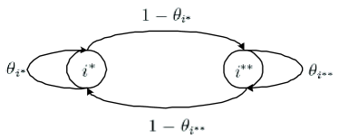
Figure 2: A Markov process representation of the optimistic strategy $\Gamma_{SW}^{*}$.

The probability $P_{i^{**}}$ that the cognitive user will sense channel $i^{**}$ can be obtained by the solving the following stationary equation

$$P_{i^{**}}=(1-\theta_{i^{*}})(1-P_{i^{**}})+\theta_{i^{**}}P_{i^{**}},$$

from which we obtain

$$P_{i^{**}}=\frac{1-\theta_{i^{*}}}{1-\theta_{i^{*}}+1-\theta_{i^{**}}}.$$

Hence in the nontrivial cases, we have

$$L(\hbox{\boldmath$\theta$};\Gamma_{SW}^{*})=BP_{i^{**}}(\theta_{i^{*}}-\theta_{i^{**}})T,$$

implying that, for any switching rule, $L(\hbox{\boldmath$\theta$};\Gamma_{SW})\sim O(T)$. ∎

There are several strategies that have loss of order $O(\ln T)$. We adopt the following linear complexity strategy which was proposed and analyzed in [18].

Rule 1

(Order optimal single index strategy)

The cognitive user maintains two vectors $\mathbf{X}$ and $\mathbf{Y}$, where each $X_{i}$ records the number of time slots for which the cognitive user has sensed channel $i$ to be free, and each $Y_{i}$ records the number of time slots for which the cognitive user has chosen channel $i$ to sense. The strategy works as follows.

1. Initialization: at the beginning of each block, sense each channel once.

2. After the initialization period, the cognitive user obtains an estimation $\hat{\hbox{\boldmath$\theta$}}$ at the beginning of time slot $j$, given by

   $$\hat{\theta}_{i}(j)=\frac{X_{i}(j)}{Y_{i}(j)},$$

   and assigns an index

   $$\Lambda_{i}(j)=\hat{\theta}_{i}(j)+\sqrt{\frac{2\ln j}{Y_{i}(j)}}$$

   to the $i^{th}$ channel. The cognitive user chooses the channel with the largest value of $\Lambda_{i}(j)$ to sense at time slot $j$. After each sensing, the cognitive user updates $\mathbf{X}$ and $\mathbf{Y}$.

The intuition behind this strategy is that as long as $Y_{i}$ grows as fast as $O(\ln T)$, $\Lambda_{i}$ converges to the true value of $\theta_{i}$ in probability, and the cognitive user will choose the channel with the largest $\theta_{i}$ eventually. The loss of $O(\ln T)$ comes from the time spent on sampling the inferior channels in order to learn the value of $\theta$. This price, however, is inevitable as established in the lower bound of Lemma 4.∎

Finally, we observe that the difference between the myopic rule and the order optimal single index rule is the additional term $\sqrt{2\ln j/Y_{i}(j)}$ added to the current estimate $\hat{\theta}_{i}$. Roughly speaking, this additional term guarantees enough sampling time for each channel, since if we sample channel $i$ too sparsely, $Y_{i}(j)$ will be small, which will increase the probability that $\Lambda_{i}$ is the largest index. When $Y_{i}(j)$ scales as $\ln T$, $\hat{\theta}_{i}$ will be the dominant term in the index $\Lambda_{i}$, and hence the channel with the largest $\theta_{i}$ will be chosen much more frequently.

IV Multi User–Single Channel

The presence of multiple cognitive users adds an element of competition to the problem. In order for a cognitive user to get hold of a channel now, it must be free from the primary traffic and the other competing cognitive users. More rigorously, we assume the presence of a set $\mathcal{K}=\{1,\cdots,K\}$ of cognitive users and consider the distributed medium access decision processes at the multiple users with no prior coordination. We denote $\mathcal{K}_{i}(j)\subseteq\mathcal{K}$ as the random set of users who choose to sense channel $i$ at time slot $j$. We assume that the users follow a generalized version of the Carrier Sense Multiple Access/Collision Avoidance (CSMA-CA) protocol to access the channel after sensing the main channel to be free, i.e., if channel $i$ is free, each user $k$ in the set $\mathcal{K}_{i}(j)$ will generate a random number $t_{k}(j)$ according to a certain probability density function $g$, and wait the time specified by the generated random number. At the end of the waiting period, user $k$ senses the channel again, and if it is found free, the packet from user $k$ will be transmitted. The probability that user $k$ in the set $\mathcal{K}_{i}(j)$ gains access to the channel is the same as the probability that $t_{k}(j)$ is the smallest random number generated by the users in the set $\mathcal{K}_{i}(j)$. Thus, the throughput user $k$ achieves in a block is

$$W_{k}=\sum\limits_{j=1}^{T}BZ_{S_{k}(j)}(j)I\left\{k=\arg\min\limits_{q\in\mathcal{K}_{S_{k}(j)}(j)}t_{q}(j)\right\}.$$

Therefore, user $k$ should devise sensing rule $\Gamma_{k}$ that maximizes

$$\mathbb{E}\left\{W_{k}\right\}=\mathbb{E}\left\{\sum\limits_{j=1}^{T}BZ_{S_{k}(j)}(j)I\left\{k=\arg\min\limits_{q\in\mathcal{K}_{S_{k}(j)}(j)}t_{q}(j)\right\}\right\}.$$

Clearly, with multiple cognitive users, it is not optimal anymore for all the users to always choose the channel with the largest $\theta_{i}$ to sense. In particular, if all the users choose the channel with the largest $\theta_{i}$, the probability that a given user gains control of the channel decreases, while potential opportunities in the other channels in the primary network are wasted.

IV-A Known $\theta$ Case

To enable a succinct presentation, we first consider the case in which the values of $\theta$ are known to all the cognitive users. The users distributively choose channels to sense and compete for access if the channels are free.

IV-A1 The Optimal Symmetric Strategy

Without loss of generality, we consider a mixed strategy where user $k$ will choose channel $i$ with probability $p_{k,i}$. Furthermore, we let $\mathbf{p}_{k}=[p_{k,1},\cdots,p_{k,N}]$ and consider the symmetric solution in which $\mathbf{p}=\mathbf{p}_{1}=\cdots=\mathbf{p}_{K}$. The symmetry assumption implies that all the users in the network distributively follow the same rule to access the spectral opportunities present in the primary network, in order to maximize the same average throughput each user can obtain. The following result derives the optimal solution in this situation.

Lemma 6

For a cognitive network with $K>1$ cognitive users and $N$ channels with probability $\theta$ of being free, the optimal $\mathbf{p}^{*}$ is given by

$$p_{i}^{*}=\left\{\begin{array}[]{ll}\left\{1-\left(\frac{\lambda^{*}}{K\theta_{i}}\right)^{1/(K-1)}\right\}^{+},&\quad\text{for}\quad\theta_{i}>0,\\ 0,&\quad\text{for}\quad\theta_{i}=0,\end{array}\right.$$ (14)

where $\lambda^{*}$ is a constant such that $\sum\limits_{i=1}^{N}p_{i}^{*}=1$. Here $\{x\}^{+}=\max\{0,x\}$.

Proof:

With a strategy $\mathbf{p}$, the probability that user $k$ chooses channel $i$ and, at the same time, there are $l$ other users choosing channel $i$ to sense is

$$p_{i}{{K-1}\choose l}p_{i}^{l}(1-p_{i})^{K-1-l}.$$

Under this scenario, the average bits transmitted at one slot of each user is $B\theta_{i}/(l+1)$, Hence, the average throughput $W_{k}$ of user $k$ is

$$W_{k}=T\sum\limits_{i=1}^{N}\frac{B\theta_{i}}{l+1}\sum\limits_{l=0}^{K-1}p_{i}{{K-1}\choose l}p_{i}^{l}(1-p_{i})^{K-1-l}.$$

Based on our symmetry assumption, we drop the subscript $k$ and write the average throughput of each user as $W$ leading to

$$W = BT\sum\limits_{i=1}^{N}p_{i}\theta_{i}\sum\limits_{l=0}^{K-1}{{K-1}\choose l}\frac{p_{i}^{l}(1-p_{i})^{K-1-l}}{l+1}$$

$$= BT\sum\limits_{i=1}^{N}p_{i}\theta_{i}\sum\limits_{l=0}^{K-1}\frac{(K-1)!}{l!(K-1-l)!}\frac{p_{i}^{l}(1-p_{i})^{K-1-l}}{l+1}$$

$$= BT\sum\limits_{i=1}^{N}\frac{\theta_{i}}{K}\sum\limits_{l=0}^{K-1}{K\choose{l+1}}p_{i}^{l+1}(1-p_{i})^{K-1-l}$$

$$= BT\sum\limits_{i=1}^{N}\frac{\theta_{i}}{K}\left\{\sum\limits_{l^{{}^{\prime}}=0}^{K}{K\choose l^{{}^{\prime}}}p_{i}^{l^{{}^{\prime}}}(1-p_{i})^{K-l^{{}^{\prime}}}-(1-p_{i})^{K}\right\}$$

$$= BT\sum\limits_{i=1}^{N}\frac{\theta_{i}}{K}\left\{1-(1-p_{i})^{K}\right\}.$$

Now, we should solve the following optimization problem

$$\max\quad W=BT\sum\limits_{i=1}^{N}\frac{\theta_{i}}{K}\left\{1-(1-p_{i})^{K}\right\},$$

s.t. $$\sum\limits_{i=1}^{N}p_{i}=1,$$

$$\mathbf{p}\geq\mathbf{0}.$$

This optimization problem is equivalent to the following:

$$\min\quad y=\sum\limits_{i=1}^{N}\theta_{i}(1-p_{i})^{K},$$

s.t. $$\sum\limits_{i=1}^{N}p_{i}=1,$$

$$\mathbf{p}\geq\mathbf{0}.$$

Since

$$\frac{\partial^{2}y}{\partial^{2}p_{i}}=\theta_{i}K(K-1)(1-p_{i})^{K-2}\geq 0,$$

for $0\leq p_{i}\leq 1$, $y$ is a convex function of $\mathbf{p}$ in the region of interest, i.e. $\mathbf{p}\in[0,1]^{N}$. Also, the constraints are the intersection of a convex set and a linear constraint. Therefore, our problem reduces to a convex optimization problem whose Karush-Kuhn-Tucker (KKT) conditions[19] for optimality are

$$\mathbf{p}^{*} \geq \mathbf{0},$$

$$\sum\limits_{i=1}^{N}p^{*}_{i} = 1,$$

$$p_{i}^{*}\left(\lambda^{*}-K\theta_{i}(1-p_{i}^{*})^{K-1}\right) = 0,$$

$$\lambda^{*} \geq K\theta_{i}(1-p_{i}^{*})^{K-1},$$

where $\lambda^{*}$ is the Lagrange multiplier.

It is easy to check that if $K>1$,

$$p_{i}^{*}=\left\{\begin{array}[]{ll}\left\{1-\left(\frac{\lambda^{*}}{K\theta_{i}}\right)^{1/(K-1)}\right\}^{+}&\quad\text{for}\quad\theta_{i}>0,\\ 0&\quad\text{for}\quad\theta_{i}=0,\end{array}\right.$$ (18)

satisfies the KKT conditions, in which $\lambda^{*}$ is the constant that satisfies $\sum p_{i}^{*}=1$. ∎

If $K=1$, then $p_{i^{*}}^{*}=1$, where $i^{*}=\arg\max\limits_{i\in\mathcal{N}}\theta_{i}$, $p_{l}^{*}=0$, and $l\in\mathcal{N}\backslash\{i^{*}\}$, satisfies the KKT conditions.

So, the total throughput of the $K$ cognitive users is

$$KW = BKT\sum\limits_{i=1}^{N}\frac{\theta_{i}}{K}\left\{1-(1-p_{i}^{*})^{K}\right\}$$

$$= BT\sum\limits_{i=1}^{N}\theta_{i}\left\{1-(1-p_{i}^{*})^{K}\right\}.$$

On the other hand, the average total spectral opportunities of the primary network is $BT\sum\limits_{i=1}^{N}\theta_{i}$. This upper bound can be achieved by a centralized channel allocation strategy when $K>N$ (simply by assigning one cognitive user to each channel). Therefore, the loss of the distributed protocol as compared with the centralized scheduling is

$$L=BT\sum\limits_{i=1}^{N}\theta_{i}(1-p_{i}^{*})^{K},$$

which is same as (IV-A1) up to a constant factor. There is an intuitive explanation of this loss. If there is a spectral opportunity in channel $i$ but there are no users choosing channel $i$ to sense, a loss occurs. The probability that there is no user choosing channel $i$ to sense is $(1-p_{i}^{*})^{K}$, and hence the probability of loss occurring at channel $i$ is $\theta_{i}(1-p_{i}^{*})^{K}$. To obtain further insights on the performance of the cognitive network, we study the following special cases.

1. $N\geq 1,K=1$. As stated in the above, $p_{i^{*}}^{*}=1$, and $p_{l}^{*}=0,l\in\mathcal{N}\backslash\{i^{*}\}$. Hence, the user should choose the channel with the largest free probability to sense. And

   $$L=BT\sum\limits_{i\in\mathcal{N}\backslash\{i^{*}\}}\theta_{i}.$$

2. $N=2,K=2$. Substituting $N=2$ and $K=2$ into (18), we obtain

   $$p_{1}^{*}=\theta_{1}/(\theta_{1}+\theta_{2})\quad\text{and}\quad p_{2}^{*}=\theta_{2}/(\theta_{1}+\theta_{2}).$$

   Furthermore,

   $$W = \frac{BT\theta_{1}}{2}\left[1-\frac{\theta_{2}^{2}}{(\theta_{1}+\theta_{2})^{2}}\right]$$

   $$+\frac{BT\theta_{2}}{2}\left[1-\frac{\theta_{1}^{2}}{(\theta_{1}+\theta_{2})^{2}}\right],$$

   $$L = \frac{BT\theta_{1}\theta_{2}}{2(\theta_{1}+\theta_{2})}.$$

3. $N$ is fixed, and $K\rightarrow\infty$. We have the following asymptotic characterization.

Lemma 7

Let $2\leq Q\leq N$ be the number of channels for which $\theta_{i}>0$. We have $p_{i}^{*}\rightarrow 1/Q$, and $L\rightarrow 0$ exponentially as $K$ increases, i.e.,

$$L\sim O(e^{-c_{1}K}),$$

where $c_{1}=\ln\frac{Q}{Q-1}$.

Proof:

Without loss of generality, we assume that $\theta_{i}\neq 0$, for $1\leq i\leq Q$. At the moment, we assume that (we will show that this is true, if $K$ is large enough) if $\theta_{i}\neq 0$

$$p_{i}^{*}=\left\{1-\left(\frac{\lambda^{*}}{K\theta_{i}}\right)^{1/(K-1)}\right\}^{+}=1-\left(\frac{\lambda^{*}}{K\theta_{i}}\right)^{1/(K-1)}.$$

Together with $\sum\limits_{i=1}^{N}p_{i}^{*}=\sum\limits_{i=1}^{Q}p_{i}^{*}=1$, we have

$$(\lambda^{*})^{1/(K-1)}=\frac{K^{1/(K-1)}(Q-1)}{\sum\limits_{i=1}^{Q}\theta_{i}^{-1/(K-1)}}$$

and

$$p_{i}^{*}=1-\frac{(Q-1)\theta_{i}^{-1/(K-1)}}{\sum\limits_{i=1}^{Q}\theta_{i}^{-1/(K-1)}},\quad\text{for}\quad 1\leq i\leq Q.$$

To satisfy the condition $\mathbf{p}\geq\mathbf{0}$, we need to show

$$\frac{(Q-1)\theta_{i}^{-1/(K-1)}}{\sum\limits_{i=1}^{Q}\theta_{i}^{-1/(K-1)}}\leq 1,$$

for all $i$ with $\theta_{i}>0$.

With $i^{*}=\arg\max\limits_{i\in\mathcal{N}}\theta_{i}$ and $l^{*}=\arg\min\limits_{1\leq l\leq Q}\theta_{l}$, we have for all $i$

$$\frac{(Q-1)\theta_{i}^{-1/(K-1)}}{\sum\limits_{i=1}^{Q}\theta_{i}^{-1/(K-1)}}\leq\frac{(Q-1)\theta_{l^{*}}^{-1/(K-1)}}{Q\theta_{i^{*}}^{-1/(K-1)}}.$$

For any $\vartheta\leq Q/(Q-1)$, if $K$ is large enough, we have

$$\left(\frac{\theta_{i^{*}}}{\theta_{l^{*}}}\right)^{\frac{1}{K-1}}\leq\vartheta$$

since

$$\lim\limits_{K\rightarrow\infty}\left(\frac{\theta_{i^{*}}}{\theta_{l^{*}}}\right)^{\frac{1}{K-1}}=1.$$

Hence, for all $1\leq i\leq Q$, we have

$$\frac{(Q-1)\theta_{i}^{-1/(K-1)}}{\sum\limits_{i=1}^{Q}\theta_{i}^{-1/(K-1)}}\leq\frac{Q-1}{Q}\vartheta\leq 1.$$

Now, straightforward limit calculation shows that

$$p^{*}\rightarrow 1/Q,$$

as $K$ increases. And

$$\lim\limits_{K\rightarrow\infty}\frac{L}{\exp^{-c_{1}K}}=\lim\limits_{K\rightarrow\infty}\frac{BT\sum\limits_{i=1}^{Q}\theta_{i}(1-p_{i}^{*})^{K}}{\exp^{-c_{1}K}}=BT\sum\limits_{i=1}^{Q}\theta_{i}$$

with $c_{1}=\ln\frac{Q}{Q-1}$. ∎

The reason for the exponential decrease in the loss is that, as the number of cognitive users increases, the probability that there is no user sensing any particular channel decreases exponentially. If $Q=1$, there is no loss of performance, since the all the user will always sense the channel with non-zero availability probability.

IV-A2 The Game Theoretic Model

The optimality of the distributed protocol proposed in the previous section hinges on the assumption that all the users will follow the symmetric rule. However, it is straightforward to see that if a single cognitive user deviates from the rule specified in Lemma 6, it will be able to transmit more bits. If this selfish perspective propagates through the network, it may lead to a significant reduction in the overall throughput. This observation motivates our next step in which the channel selection problem is modeled as a non-cooperative game, where the cognitive users are the players, the $\Gamma_{k}$s are the strategies and the average throughput of each user is the payoff. The following result derives a sufficient condition for the Nash equilibrium [20] in the asymptotic scenario $K\rightarrow\infty$.

Lemma 8

$(\Gamma_{1},\cdots,\Gamma_{K})$ is a Nash-equilibrium, if $K$ is large and at each time slot, there are $\tau_{i}K$ users sensing channel $i$, where $\tau_{i}$ satisfies

$$\tau_{i}=\frac{\theta_{i}}{\sum\limits_{i=1}^{N}\theta_{i}}.$$ (19)

At this equilibrium, each user has probability $\frac{\sum\limits_{i=1}^{N}\theta_{i}}{K}$ of transmitting at each time slot.

Proof:

We prove this by backward induction. At the last time slot $T$, if $\tau_{i}$s satisfy equation (19), the probability of user $k$ gaining a channel is

$$p_{k}=\frac{\theta_{i}}{\tau_{i}K}=\frac{\sum\limits_{i=1}^{N}\theta_{i}}{K}.$$

Now, if user $k$ deviates from this strategy, and chooses channel $i^{{}^{\prime}}$, the number of users sensing channel $i^{{}^{\prime}}$ is $\tau_{i^{{}^{\prime}}}K+1$, and the probability of user $k$ gaining the channel is

$$p_{k}^{{}^{\prime}}=\frac{\theta_{i^{{}^{\prime}}}}{\tau_{i^{{}^{\prime}}}K+1}<\frac{\theta_{i^{{}^{\prime}}}}{\tau_{i^{{}^{\prime}}}K}=p_{k}.$$

Hence the strategy that has $\tau_{i}K$ users sensing channel $i$ at time slot $T$ is a Nash equilibrium. Now, we know the optimal strategy for the last time-slot, so we can ignore this time slot. Then time slot $T-1$ becomes the last slot, in which this strategy is optimal. Similarly, we show that this strategy is optimal for all other time slots. ∎

We note that in the lemma we implicitly assume that $\tau_{i}K$ is an integer. In practice, this is not always true. However, since $K$ is large, rounding $\tau_{i}K$ to the nearest integer will have minor effects. The Nash equilibrium is also optimal from a system perspective, in the sense that this strategy maximizes the total throughput of the whole network by fully utilizing the available spectral opportunities when $K$ is large (i.e., on the average, each user will be able to transmit $\frac{BT\sum\theta_{i}}{K}$ bits per block, and the total throughput of the network is $BT\sum\theta_{i}$).

With this equilibrium result, the cognitive users can use the following stochastic sensing strategy to approximately work on the equilibrium point for a large but finite $K$. Let $s_{k}(j)$ be the channel chosen by user $k$ at time slot $j$. At each time slot, each user independently selects channel $i$ with probability $\tau_{i}=\frac{\theta_{i}}{\sum\limits_{i\in\mathcal{N}}\theta_{i}}$, i.e., $\text{Pr}\{s_{k}(j)=i\}=\tau_{i}$. Then at each time slot, the number of users sensing channel $i$ will be $\sum\limits_{k=1}^{K}I\{s_{k}(j)=i\}$, where the $I\{s_{k}(j)=i\}$s are i.i.d Bernoulli random variables. Hence, the total number of users sensing channel $i$ is a binomial random number, and the fraction of users sensing channel $i$ converges to $\tau_{i}$ in probability as $K$ increases, i.e.

$$\tau^{{}^{\prime}}=\frac{\sum\limits_{k=1}^{K}I\{s_{k}(j)=i\}}{K}\rightarrow\tau_{i}$$

in probability. Hence, as $K$ increases, the operating point will converge to the Nash equilibrium in probability.

For any $K$, the probability that there is no user choosing channel $i$ to sense is $(1-\tau_{i})^{K}$. Hence the performance loss compared with the centralized scheme is

$$L=BT\sum\theta_{i}(1-\tau_{i})^{K}=BT\sum\limits_{i=1}^{N}\theta_{i}\left(\frac{\sum_{l=1}^{N}\theta_{l}-\theta_{i}}{\sum_{l=1}^{N}\theta_{l}}\right)^{K}.$$

It is easy to check that

$$\lim\limits_{K\rightarrow\infty}\frac{L}{\exp^{-c_{2}K}}=BT\theta_{l^{*}},$$

where $\theta_{l^{*}}=\min\{\theta_{i}:\theta_{i}>0\}$, and $c_{2}=\ln\frac{\sum\theta_{i}}{\sum_{l=1}^{N}\theta_{l}-\theta_{l^{*}}}$. It is now clear that the loss of the game theoretic scheme goes to zero exponentially, though the decay rate is smaller than that of the scheme specified in Lemma 6. On the other hand, compared with the scheme in Lemma 6, the game theoretic scheme has the advantage that the individual cognitive users do not need to know the total number of cognitive users $K$ in the network and, more importantly, they have no incentive to deviate unilaterally.

IV-B Unknown $\theta$ Case

If $\theta$ is unknown, the cognitive users need to estimate $\theta$ (in addition to resolving their competition). Combining the results from Sections III-B and IV-A, we design the following low complexity strategy which is asymptotically optimal.

Rule 2

1) Initialization: Each user $k$ maintains the following two vectors: $\mathbf{X}_{k}$, which records the number of time slots in which user $k$ has sensed each channel to be free; and $\mathbf{Y}_{k}$, which records the number of time slots in which user $k$ has sensed each channel. At the beginning of each block, user $k$ senses each channel once and transmits through this channel if the channel is free and it wins the competition. Also, set $X_{k,i}=1$, regardless of the sensing result of this stage.

2) At the beginning of time slot $j$, user $k$ estimates $\hat{\theta}_{i}$ as

$$\hat{\theta}_{i}(j)=X_{k,i}(j)/Y_{k,i}(j),$$

and chooses each channel $i\in\mathcal{N}$ with probability

$$\frac{\hat{\theta}_{i}(j)}{\sum\limits_{i=1}^{N}\hat{\theta}_{i}(j)}.$$ (20)

After each sensing, $\mathbf{X}_{k}$ and $\mathbf{Y}_{k}$ are updated.∎

Lemma 9

If $K$ is large, the scheme in Rule 2 converges to the Nash equilibrium specified in Lemma 8 in probability, as $T$ increases.

Proof:

$X_{k,i}$ is the sum of $Y_{k,i}$ i.i.d Bernoulli random variables with parameter $\theta_{i}$. We use the following form of the Chernoff bound. Let $X$ be the sum of $n$ independent Bernoulli random variables with parameter $\bar{\theta}$, then

$$\text{Pr}\left\{X\leq(1-\delta)n\bar{\theta}\right\}<\exp\left(\frac{-n\bar{\theta}\delta^{2}}{2}\right)$$

for any $\delta<1$.

At time slot $j$, if we replace $X$ with $X_{k,i}(j)$, $n$ with $Y_{k,i}(j)$, $\bar{\theta}$ with $\theta_{i}$ and let $\delta=1/2$, then we have

$$\text{Pr}\left\{X_{k,i}(j)\leq\frac{1}{2}\theta_{i}Y_{k,i}(j)\right\}<\exp\left(-Y_{k,i}(j)\theta_{i}/8\right).$$

Hence

$$\text{Pr}\left\{\frac{X_{k,i}(j)}{Y_{k,i}(j)}\geq\frac{\theta_{i}}{2}\right\} \geq 1-\exp\left(-Y_{k,i}(j)\theta_{i}/8\right)$$ (21)

$$\geq 1-\exp\left(-\theta_{i}/8\right),$$

since after the initialization period, $Y_{k,i}(j)\geq 1$.

Note that $Y_{k,i}(T)$ is the total number of time slots that user $k$ has sensed channel $i$ in each block with $T$ time slots. We have

$$\mathbb{E}\{Y_{k,i}(T)\} = \mathbb{E}\left\{\sum\limits_{j=1}^{T}I\left\{S_{k}(j)=i\right\}\right\}$$

$$= \sum\limits_{j=1}^{T}\mathbb{E}\left\{I\left\{S_{k}(j)=i\right\}\right\}$$

$$= \sum\limits_{j=1}^{T}\mathbb{E}\left\{\frac{X_{k,i}(j)/Y_{k,i}(j)}{\sum\limits_{i\in\mathcal{N}}X_{k,i}(j)/Y_{k,i}(j)}\right\}$$

$$\overset{(a)}{\geq} \sum\limits_{j=1}^{T}\mathbb{E}\left\{\frac{X_{k,i}(j)/Y_{k,i}(j)}{N}\right\}$$

$$\overset{(b)}{\geq} \sum\limits_{j=1}^{T}\frac{\theta_{i}(1-\exp(-\theta_{i}/8))}{2N}$$

$$= T\frac{\theta_{i}}{2N}(1-\exp(-\theta_{i}/8))=c_{i}T,$$

where (a) follows from the fact that $X_{k,i}(j)/Y_{k,i}(j)\leq 1$, and (b) follows from (21).

The probability that $Y_{k,i}(T)\leq(1-\delta)\mathbb{E}\{Y_{k,i}(T)\}$ can also be bounded using the Chernoff bounds since $Y_{k,i}(T)$ is also the sum of independent Bernoulli random variables. In particular, we have

$$\text{Pr}\{Y_{k,i}(T)\leq(1-\delta)\mathbb{E}\{Y_{k,i}(T)\}\}\leq\exp\left(\frac{-\delta^{2}\mathbb{E}\{Y_{k,i}(T)\}}{2}\right).$$

On letting

$$\delta=\sqrt{\frac{\ln\mathbb{E}\{Y_{k,i}(T)\}}{\mathbb{E}\{Y_{k,i}(T)\}}},$$

we have

$$\text{Pr}\left\{Y_{k,i}(T)\leq\mathbb{E}\{Y_{k,i}(T)\}-\ln\mathbb{E}\{Y_{k,i}(T)\}\right\}\leq\frac{1}{c_{i}T}.$$

Using the union bound, and the weak law of large numbers, $X_{k,i}(j)/Y_{k,i}(j)$ converges to $\theta_{i}$ in probability as $T$ increases (with probability larger than $1-1/T$). The scheme becomes the same as the known $\theta$ case, in which we know that the operating point is approximately at the Nash equilibrium, if $K$ is sufficiently large. ∎

The intuition behind this scheme is that, each user will sample each channel at least $O(T)$ times, and hence as $T$ increases, the estimate $\hat{\hbox{\boldmath$\theta$}}$ converges to $\theta$ in probability implying that the unknown $\theta$ case will eventually reduce to the case in which $\theta$ is known to all the users. Hence, if $K$ is sufficiently large, the operating point converges to the Nash equilibrium in probability.

If one can assume that the users will follow the pre-specified rule, then we can design the following strategy that converges to the optimal operating point in probability for any $K$, as $T$ increases.

Rule 3

1) Initialization: Each user $k$ maintains the following two vectors: $\mathbf{X}_{k}$, which records the number of time slots in which user $k$ has sensed each channel to be free, $\mathbf{Y}_{k}$, which records the number of time slots in which user $k$ has sensed each channel. At the beginning of each block, user $k$ senses each channel once, and transmits through this channel if the channel is free and it wins the competition. Also, set $X_{k,i}=1$, regardless of what the sensing result at this stage.

2) At the beginning of time slot $j\leq\ln T$, user $k$ estimates $\hat{\theta}_{i}$ as

$$\hat{\theta}_{i}(j)=X_{k,i}(j)/Y_{k,i}(j),$$

and chooses each channel $i\in\mathcal{N}$ with probability $\hat{\theta}_{i}(j)/\sum\limits_{i=1}^{N}\hat{\theta}_{i}(j)$. For $j\geq\ln T$, the $i^{th}$ channel is sensed with probability

$$\hat{p}_{i}^{*}=\left\{1-\left(\frac{\lambda^{*}}{\hat{\theta_{i}}}\right)^{1/(K-1)}\right\}^{+}.$$ (22)

After each sensing, $\mathbf{X}_{k}$ and $\mathbf{Y}_{k}$ are updated.∎

Lemma 10

The proposed scheme converges in probability to the optimal operating point specified in Lemma 6, as $T$ increases.

Proof:

Following the same steps as the proof of Lemma 9, one can show that after $O(\ln T)$ times slots, $\hat{\hbox{\boldmath$\theta$}}$ converges to $\theta$ in probability as $T$ increases. Hence the operating point specified by (22) converges in probability to the optimal point specified in Lemma 6 as $T$ increases. ∎

V Multi-Channel Cognitive Users

In certain scenarios, cognitive users may be able to sense more than one channel simultaneously. To simplify the presentation, we assume the presence of only a single cognitive user capable of sensing, and subsequently utilizing, $M\leq N$ channels simultaneously. Let $\mathcal{M}(j)$ be the set of channels the cognitive user selects to sense at time slot $j$, where $|\mathcal{M}(j)|=M$. The average number of bits that the cognitive user is able to send over a block is therefore

$$\mathbb{E}\{W\}=\mathbb{E}\left\{\sum\limits_{j=1}^{T}\sum\limits_{S(j)\in\mathcal{M}(j)}BZ_{S(j)}(j)\right\}.$$

At the beginning of time slot $j$, the cognitive user can update the pdf $f^{j}(\hbox{\boldmath$\theta$})$ according to (3) and (4). Similar to Lemma 1, the optimal solution can be characterized by the following optimality condition

$$V^{*}(f,T) = \max\limits_{\mathcal{M}(1)\subseteq\mathcal{N},|\mathcal{M}(1)|=M}\mathbb{E}_{f}\Bigg{\{}\sum\limits_{s(1)\in\mathcal{M}(1)}BZ_{s(1)}$$ (23)

$$\hskip 11.38109pt+V^{*}\left(f_{\{Z_{s(1)}:s(1)\in\mathcal{M}(1)\}},T-1\right)\Bigg{\}}.$$

Here, $f_{\{Z_{s(1)}:s(1)\in\mathcal{M}(1)\}}$ is the updated density after observing the sensing output of the channels $s(1)\in\mathcal{M}(1)$. We can then follow the same procedure described for the single-channel sensing scenario to obtain the optimal strategy $\Gamma^{*}$ according to (23). In the following, however, we focus on low complexity non-parametric strategies that are asymptotically optimal.

If $\theta$ is known, the cognitive user will choose the $M$ channels with the largest $\theta$’s to sense. Without loss of generality, we assume $\theta_{1}\geq\theta_{2}\geq\cdots\geq\theta_{N}$. Hence, for any strategy $\Gamma$, the loss is

$$L(\hbox{\boldmath$\theta$};\Gamma)=\sum\limits_{j=1}^{T}\sum\limits_{i=1}^{M}B\theta_{i}-\sum\limits_{j=1}^{T}B\sum\limits_{i=1}^{N}\theta_{i}P\left\{i\in\mathcal{M}(j)\right\},$$

We have the following order-optimal simple single-index strategy.

Rule 4

The cognitive user maintains two vectors $\mathbf{X}$ and $\mathbf{Y}$, where each $X_{i}$ is the number of time slots in which the cognitive user has sensed channel $i$ to be free, and each $Y_{i}$ is the number of time slots in which the cognitive user has chosen channel $i$ to sense. The strategy works as follows.

1. Initialization: at the beginning of each block, each channel is sensed once. This initialization stage takes $\lceil N/M\rceil$ time slots, in which $\lceil x\rceil$ denotes the least positive integer that is no less than $x$.

2. After the initialization period, the cognitive user obtains an estimation $\hat{\hbox{\boldmath$\theta$}}$ at the beginning of time slot $j$ given by

   $$\hat{\theta}_{i}(j)=\frac{X_{i}(j)}{Y_{i}(j)},$$

   and assigns an index

   $$\Lambda_{i}(j)=\hat{\theta}_{i}(j)+\sqrt{\frac{2\ln j}{Y_{i}(j)}}$$

   to the $i^{th}$ channel. The cognitive user orders these $\Lambda_{i}(j)$s and selects the $M$ channels with the largest $\Lambda_{i}(j)$s to sense. After each sensing, the cognitive user updates $\mathbf{X}$ and $\mathbf{Y}$.

Lemma 11

Rule 4 is asymptotically optimal and $L(\hbox{\boldmath$\theta$},\Gamma)\sim O(\ln T).$

Proof:

We bound $Y_{i}(T)$ for $i\geq M+1$, i.e., the channels that are not among the channels having the $M$ largest values of $\theta$. Note that $Y_{i}(T)$ is the total number of time slots in which the cognitive user has sensed channel $i$ in a block with $T$ time slots. We have

$$Y_{i}(T) = 1+\sum\limits_{j=\lceil N/M\rceil+1}^{T}I\left\{i\in\mathcal{M}(j)\right\}$$

$$\leq m+\sum\limits_{j=\lceil N/M\rceil+m}^{T}I\left\{i\in\mathcal{M}(j)\Big{|}Y_{i}(j)\geq m\right\},$$

for any $m\geq 1$, where $I\{x|y\}$ is the conditional indicator function, which equals 1 if, conditioning on $y$, $x$ is satisfied, and otherwise equals 0. Since $Y_{i}(j)\geq m$, it follows that $i\in\mathcal{M}(j)$ only if $\Lambda_{i}(j)$ is among the $M$ largest indices. Hence, a necessary condition for $i\in\mathcal{M}(j)$ is

$$\Lambda_{i}(j)\geq\min\{\Lambda_{l}(j):1\leq l\leq M\}.$$

Otherwise, if

$$\Lambda_{i}(j)<\min\{\Lambda_{l}(j):1\leq l\leq M\},$$

then the indices of these $M$ channels are already larger than that of channel $i$, and channel $i$ will not be selected. Thus

$$I\left\{i\in\mathcal{M}(j)\Big{|}Y_{i}(j)\geq m\right\}$$

$$\leq I\left\{\Lambda_{i}(j)\geq\min\{\Lambda_{l}(j):1\leq l\leq M\}\Big{|}Y_{i}(j)\geq m\right\}$$

$$\leq \sum\limits_{l=1}^{M}I\left\{\Lambda_{i}(j)\geq\Lambda_{l}(j)\Big{|}Y_{i}(j)\geq m\right\}.$$

Hence

$$Y_{i}(T) \leq m+\sum\limits_{j=\lceil N/M\rceil+m}^{T}\sum\limits_{l=1}^{M}I\left\{\Lambda_{i}(j)\geq\Lambda_{l}(j)\Big{|}Y_{i}(j)\geq m\right\}$$

$$\leq \sum\limits_{l=1}^{M}\left\{m+\sum\limits_{j=\lceil N/M\rceil+m}^{T}I\left\{\Lambda_{i}(j)\geq\Lambda_{l}(j)\Big{|}Y_{i}(j)\geq m\right\}\right\}.$$

In order for $\Lambda_{i}(j)\geq\Lambda_{l}(j)$, one of the following three conditions must be satisfied

$$\Lambda_{l}(j)\leq\theta_{l},\;\Lambda_{i}(j)\geq\theta_{i}+2\sqrt{\frac{2\ln j}{Y_{i}(j)}},\;\text{or}\;\theta_{l}\leq\theta_{i}+2\sqrt{\frac{2\ln j}{Y_{i}(j)}}.$$

One can easily check that, if none of these three conditions is satisfied, we will have $\Lambda_{i}(j)<\Lambda_{l}(j)$. In the following, we bound the probability of each event.

$$\text{Pr}\left\{\Lambda_{l}(j)\leq\theta_{l}\Big{|}Y_{i}(j)\geq m\right\}$$

$$= \text{Pr}\left\{\hat{\theta}_{l}+\sqrt{\frac{2\ln j}{Y_{l}(j)}}\leq\theta_{l}\Bigg{|}Y_{i}(j)\geq m\right\}$$

$$\leq \text{Pr}\left\{\Big{|}\hat{\theta}_{l}-\theta_{l}\Big{|}\geq\sqrt{\frac{2\ln j}{Y_{l}(j)}}\Bigg{|}Y_{i}(j)\geq m\right\}$$

$$= \sum\limits_{q=1}^{j}\text{Pr}\{Y_{l}(j)=q\}$$

$$\hskip 17.07164pt\text{Pr}\left\{\Big{|}\hat{\theta}_{l}-\theta_{l}\Big{|}\geq\sqrt{\frac{2\ln j}{Y_{l}(j)}}\Bigg{|}Y_{i}(j)\geq m,Y_{l}(j)=q\right\}$$

$$\leq \sum\limits_{q=1}^{j}\text{Pr}\left\{\Big{|}\hat{\theta}_{l}-\theta_{l}\Big{|}\geq\sqrt{\frac{2\ln j}{Y_{l}(j)}}\Bigg{|}Y_{l}(j)=q\right\}$$

$$\leq 2j\exp^{-4\ln j}$$

$$= 2j^{-3},$$

where (V) follows from to the following Chernoff-Hoeffding bounds, which says that for $n$ i.i.d Bernoulli random variables $X_{j},j=1,\cdots,n$ with mean $\bar{\theta}$,

$$\text{Pr}\left\{\left|\frac{\sum X_{j}}{n}-\bar{\theta}\right|\geq\epsilon\right\}\leq 2\exp^{-2n\epsilon^{2}},\text{ for all }\epsilon>0.$$ (25)

To see this, we note that in our case, $X_{l}(j)$ is the sum of $Y_{l}(j)$ i.i.d Bernoulli random variables with parameter $\theta_{l}$. On setting

$$n=Y_{l}(j),\;\text{and}\;\epsilon=\sqrt{\frac{2\ln j}{Y_{l}(j)}},$$

also using the fact that

$$\hat{\theta}_{l}=\frac{\sum Z_{l}(j)}{Y_{l}(j)},$$

we have (V).

Similarly, we have

$$\text{Pr}\left\{\Lambda_{i}(j)\geq\theta_{i}+2\sqrt{\frac{2\ln j}{Y_{i}(j)}}\Bigg{|}Y_{i}(j)\geq m\right\}$$

$$= \text{Pr}\left\{\hat{\theta}_{i}\geq\theta_{i}+\sqrt{\frac{2\ln j}{Y_{i}(j)}}\Bigg{|}Y_{i}(j)\geq m\right\}$$

$$= \sum\limits_{q=m}^{j}\text{Pr}\{Y_{i}(j)=q\}$$

$$\hskip 17.07164pt\text{Pr}\left\{\hat{\theta}_{i}\geq\theta_{i}+\sqrt{\frac{2\ln j}{Y_{i}(j)}}\Bigg{|}Y_{i}(j)\geq m,Y_{i}(j)=q\right\}$$

$$\leq \sum\limits_{q=1}^{j}\text{Pr}\left\{\hat{\theta}_{i}\geq\theta_{i}+\sqrt{\frac{2\ln j}{Y_{i}(j)}}\Bigg{|}Y_{i}(j)=q\right\}$$

$$\leq 2j\exp^{-4\ln j}$$

$$= 2j^{-3}.$$

At the same time, if we set

$$m=\left\lceil\frac{8\ln T}{(\theta_{i}-\theta_{M})^{2}}\right\rceil,$$

we have for any $1\leq l\leq M$, if $Y_{i}(j)\geq m$

$$\theta_{i}+2\sqrt{\frac{2\ln j}{Y_{i}(j)}}\leq\theta_{i}+2\sqrt{\frac{2\ln j}{m}}$$

$$\hskip 11.38109pt\leq\theta_{i}+(\theta_{M}-\theta_{i})\sqrt{\frac{\ln j}{\ln T}}<\theta_{M}\leq\theta_{l}.$$

Hence with this $m$,

$$\text{Pr}\left\{\theta_{l}\leq\theta_{i}+2\sqrt{\frac{2\ln j}{Y_{i}(j)}}\Bigg{|}Y_{i}(j)\geq m\right\}=0,$$

for each $1\leq l\leq M$.

Thus,

$$\text{Pr}\left\{\Lambda_{i}(j)\geq\Lambda_{l}(j)\Big{|}Y_{i}(j)\geq m\right\}$$

$$\leq \text{Pr}\left\{\Lambda_{l}(j)\leq\theta_{l}\Big{|}Y_{i}(j)\geq m\right\}$$

$$+\text{Pr}\left\{\Lambda_{i}(j)\geq\theta_{i}+2\sqrt{\frac{2\ln j}{Y_{i}(j)}}\Bigg{|}Y_{i}(j)\geq m\right\}$$

$$+\text{Pr}\left\{\theta_{l}\leq\theta_{i}+2\sqrt{\frac{2\ln j}{Y_{i}(j)}}\Bigg{|}Y_{i}(j)\geq m\right\}$$

$$\leq 4j^{-3}.$$

$$\mathbb{E}\{Y_{i}(T)\}$$

$$\leq\mathbb{E}\Bigg{\{}\sum\limits_{l=1}^{M}\Bigg{\{}m+$$

$$\hskip 11.38109pt\sum\limits_{j=\lceil N/M\rceil+m}^{T}I\left\{\Lambda_{i}(j)\geq\Lambda_{l}(j)\Big{|}Y_{i}(j)\geq m\right\}\Bigg{\}}\Bigg{\}}$$

$$=\sum\limits_{l=1}^{M}\Bigg{\{}\left\lceil\frac{8\ln T}{(\theta_{i}-\theta_{M})^{2}}\right\rceil+\sum\limits_{j=\lceil N/M\rceil+m}^{T}$$

$$\hskip 11.38109pt\mathbb{E}\left\{I\left\{\Lambda_{i}(j)\geq\Lambda_{l}(j)\Big{|}Y_{i}(j)\geq\left\lceil\frac{8\ln T}{(\theta_{i}-\theta_{M})^{2}}\right\rceil\right\}\right\}\Bigg{\}}$$

$$\leq M\left\{\left\lceil\frac{8\ln T}{(\theta_{i}-\theta_{M})^{2}}\right\rceil+\sum\limits_{j=\lceil N/M\rceil+m}^{T}4j^{-3}\right\}$$

$$\sim O(\ln T),$$

since

$$\sum\limits_{j=\lceil N/M\rceil+m}^{T}4j^{-3}\leq\sum\limits_{j=1}^{\infty}4j^{-3},$$

and $\sum\limits_{j=1}^{\infty}j^{-3}$ exists.

Hence from (V), we have that, for any channel that is not among the best $M$ channels, the average number of time slots for which this channel is selected is bounded by $O(\ln T)$. Thus, the loss is of order $O(\ln T)$.

On the other hand, it has been proved in [21] that for any consistent strategy,

$$\lim\inf\limits_{T\rightarrow\infty}\frac{L(\hbox{\boldmath$\theta$};\Gamma)}{\ln T}\geq c_{1},$$

with some constant $c_{1}$. This completes the proof. ∎

VI Conclusions

This work has developed a unified framework for the design and analysis of cognitive medium access based on the classical bandit problem. In the single user scenario, our formulation highlights the tradeoff between exploration and exploitation in cognitive channel selection. A linear complexity cognitive medium access algorithm, which is asymptotically optimal as $T\rightarrow\infty$, has been proposed. The multi-user setting has also been formulated, as a competitive bandit problem enabling the design of efficient and game theoretically fair medium access protocols. Finally, these ideas have been extended to the multi-channel scenario in which the cognitive user is capable of utilizing several channels simultaneously.

Our results motivate several interesting directions for future research. For example, developing optimal medium access strategies by taking sensing error into consideration and is of practical significance. Applying other powerful tools from sequential analysis to design and analyze wireless networks is a promising research direction.

References

- [1] J. Mitola, “Cognitive radio: Making software radios more personal,” IEEE Personal Communications, vol. 6, pp. 13–18, Aug. 1999.
- [2] S. Haykin, “Cognitive radio: Brain-empowered wireless communications,” IEEE Journal on Selected Areas In Communications, vol. 23, pp. 201–220, Feb. 2005.
- [3] N. Devroye, P. Mitran and V. Tarokh, “Achievable rates in cognitive radio channels,” IEEE Trans. on Information Theory, vol. 52, pp. 1813–1827, May 2006
- [4] Z. Sahinoglu and S. Tekinay, “On multimedia networks: Self-similar traffic and network performance,” IEEE Communications Magazine, vol. 37, pp. 48–52, Jan. 1999.
- [5] D. A. Berry and B. Fristedt, Bandit Problems: Sequential Allocation of Experiments. London: Chapman and Hall, 1985.
- [6] R. Sutton and A. Barto, Reinforcement Learning. Cambridge, MA: MIT Press, 1998.
- [7] A. Motamedi and A. Bahai, “Dynamic channel selection for spectrum sharing in unlicensed bands,” European Trans. on Telecommunications and Related Technologies, 2007. Submitted.
- [8] Q. Zhao, L. Tong, A. Swami, and Y. Chen, “Decentralized cognitive MAC for opportunistic spectrum access in ad hoc networks: A POMDP framework,” IEEE Journal on Selected Areas In Communications, vol. 25, pp. 589–600, April 2007.
- [9] D. Feldman, “Contributions to the “two-armed bandit” problem,” Annals of Mathematical Statistics, vol. 33, pp. 847–856, Sep. 1962.
- [10] T. A. Kelley, “A note on the Bernoulli two-armed bandit problem,” Annals of Statistics, vol. 2, pp. 1056–1062, Sep. 1974.
- [11] R. N. Bradt, S. M. Johnson, and S. Karlin, “On sequential designs for maximizing the sum of observations,” Annals of Mathematical Statistics, vol. 27, pp. 1060–1074, Dec. 1956.
- [12] Y. S. Chow, H. Robbins, and D. Siegmund, Great Expectations: The Theory of Optimal Stopping. Houghton Mifflin Company, 1971.
- [13] T. Ferguson, Optimal Stopping Times and Applications. http://www.math.ucla.edu/ tom/Stopping/Contents.html.
- [14] J. C. Gittins and D. M. Jones, “A dynamic allocation index for the sequential design of experiments,” Progress in Statistics, (Amsterdam), pp. 241–266, North-Holland, 1974.
- [15] M. N. Katehakis and A. F. Veinott, “The multi-armed bandit problem: Decomposition and computation,” Mathematics of Operations Research, vol. 12, pp. 262–268, May 1987.
- [16] T. L. Lai and H. Robbins, “Asymptotically efficient adaptive allocation rules,” Advances in Applied Mathematics, vol. 6, no. 1, pp. 4–22, 1985.
- [17] P. R. Kumar, “A survey of some results in stochastic adaptive control,” SIAM Journal on Control and Optimization, vol. 23, pp. 329–380, May 1985.
- [18] P. Auer, N. Cesa-Bianchi, and P. Fischer, “Finite-time analysis of the multiarmed bandit problem,” Machine Learning, vol. 47, pp. 235–256, 2002. Kluwer Academic Publishers.
- [19] S. Boyd, Convex Optimization. Cambridge Press, London, UK, 2004.
- [20] D. Fudenberg and J. Tirole, Game Theory. MIT Press, 1991.
- [21] V. Anantharam, P. Varaiya, and J. Walrand, “Asymptotically efficient allocation rules for the multiarmed bandit problem with multiple plays-part I: I.I.D. rewards,” IEEE Trans. on Automatic Control, vol. 32, pp. 968–976, Nov. 1987.
- [22] Y. Chen, G. Yu, Z. Zhang, H. Chen and P. Qiu, “On Cognitive Radio Networks with Opportunistic Power Control Strategies in Fading Channels”, to apperar, IEEE Trans. on Wireless Communications.
- [23] Q. Zhao and B. M. Sadler, “A Survey of Dynamic Spectrum Access,” IEEE Signal Processing Magazine, vol. 24, pp. 79–89, 2007.
- [24] S. Geirhofer, L. Tong, and B. M. Sadler, “Dynamic Spectrum Access in the Time Domain: Modeling and Exploiting Whitespace,”,IEEE Communications Magazine, pp. 66–72, May 2007.