Interference-induced splitting of resonances in spontaneous emission

Abstract

We study the resonance fluorescence from a coherently driven four-level atom in the Y-type configuration. The effects of quantum interference induced by spontaneous emission on the fluorescence properties of the atom are investigated. It is found that the quantum interference resulting from cascade emission decays of the atom leads to a splitting of resonances in the excited level populations calculated as a function of light detuning. For some parameters, interference assisted enhancement of inner sidebands and narrowing of central peaks may also occur in the fluorescence spectrum. We present a physical understanding of our numerical results using the dressed state description of the atom-light interaction.

I Introduction

The study of quantum interference effects in the spontaneous emission of excited atoms has attracted substantial attention in the literature gsa ; zhu1 ; zhu2 ; pas1 ; pas2 ; cardi ; zhou1 ; zhou2 ; gao ; keitel . The interference in spontaneous emission occurs when a pair of excited levels of an atom are coupled by the same vacuum modes to other levels. Many remarkable features have been predicted employing the mechanism of interferences in the spontaneous emission of atoms gsa ; zhu1 ; zhu2 ; pas1 ; pas2 . The early work of Agarwal on this subject demonstrated trapping of populations in the degenerate excited levels of a V-type atom gsa . For a non-degenerate V system in free space, Zhu et al. predicted the existence of a dark line in the spontaneous emission spectrum zhu1 . By considering an open V system where the excited atomic levels are coupled by a coherent field to another auxiliary level, Scully, Zhu, and coworkers showed the possibility of spectral line elimination and spontaneous emission cancellation zhu2 via quantum interference. Phase dependent spectral narrowing pas1 and pulse propagation dynamics pas2 have also been investigated using the four-level atomic model of Ref. zhu2 .

Since the fluorescence properties of a driven atomic system results from its spontaneous emission, studying the influence of interference in such processes has become an important topic of research cardi ; zhou1 ; zhou2 ; gao ; keitel . The driven V system has been shown to exhibit many interference effects such as fluorescence quenching cardi , ultranarrow spectral lines zhou1 , anticorrelated photon emissions zhou2 , enhanced squeezing in the fluorescence field gao , and collective population trapping keitel . All these effects assume an existence of non-orthogonal dipole moments of the atomic transitions for the interference to occur gsa . However, in real atomic systems, it is difficult to meet this condition. Different schemes involving cavities with preselected polarization akp1 , coherent- and dc- field induced splitting of atomic levels akp2 ; ficek have been proposed later to bypass the condition of non-orthogonal dipole moments. Further, the work on spontaneously generated interferences has been extended to four level atoms in different configurations. The resonance fluorescence spectrum of driven four level atoms in the $\Lambda$- and V- type configurations has been extensively studied by Li et al. fuli1 ; fuli2 . Recently, Antón et al. anton have examined a driven four level atom with three excited states and showed that a high population inversion may be achieved in the system due to the interference in spontaneous decay channels.

In this paper, we consider a four-level atom in the Y-type scheme (as shown in Fig. 1) which was proposed earlier for studies on two photon absorption bphou ; expt . It is assumed that the excited atomic states are near-degenerate and decay spontaneously via the same vacuum modes to the intermediate state. The atom in the intermediate state can further decay to the ground state. Since the cascade decays $(|1\rangle\rightarrow|3\rangle\rightarrow|4\rangle~{}\hbox{and}~{}|2\rangle\rightarrow|3\rangle\rightarrow|4\rangle)$ of the atom to its ground state from the two initially populated excited states lead to an emission of the same pair of photons, the quantum interference exists in decay processes. We investigate the role of the interference in the resonance fluorescence from the atom when driven by two coherent fields.

The paper is arranged as follows. In Sec. II, we present the atomic density matrix equations, describing the interaction of a Y-type atom with two coherent fields, when the presence of quantum interference in decay channels is included. The population dynamics of the driven atom in the steady state is then studied in Sec. III. In Sec. IV, we analyze the fluorescence spectrum of the atom and identify the origin of interference effects using the dressed states of the atomic system. Finally, the main results are summarized in Sec. V.

II driven Y-type atomic system and its density matrix equations

We consider (Fig.1) the four-level Y-type atom having two closely lying excited states with the energy separation $\hbar W_{12}$. In this scheme, the excited atomic states $|1\rangle$ and $|2\rangle$ decay spontaneously to the intermediate state $|3\rangle$ with rates $2\gamma_{1}$ and $2\gamma_{2}$, respectively. In addition, the atom in the intermediate state $|3\rangle$ can undergo spontaneous emissions to the ground state $|4\rangle$ with decay rate $2\gamma_{3}$. We assume that direct transitions between the excited states $|1\rangle\rightarrow|2\rangle$ and that between the excited and ground states $|1\rangle,|2\rangle\rightarrow|4\rangle$ of the atom are forbidden in the dipole approximation.

Figure 1: The level scheme of the Y-type atom driven by coherent fields.

A coherent field of frequency $\omega_{a}$ (amplitude $E_{a}$)is set to couple the upper transitions $|1\rangle,|2\rangle\leftrightarrow|3\rangle$ and another field of frequency $\omega_{b}$ (amplitude $E_{b}$) drives the lower transition $|3\rangle\leftrightarrow|4\rangle$. It is further assumed that the transition frequencies $(\omega_{13},\omega_{23})$ of the upper transitions are widely different from that of the lower transition $(\omega_{34})$. The Rabi frequencies of the atom-field interaction are represented as $\Omega_{1}=\vec{\bm{\mu}}_{13}.\vec{E}_{a}/\hbar$, $\Omega_{2}=\vec{\bm{\mu}}_{23}.\vec{E}_{a}/\hbar$, and $\Omega_{3}=\vec{\bm{\mu}}_{34}.\vec{E}_{b}/\hbar$ with $\vec{\bm{\mu}}_{mn}$ being the dipole moment of the atomic transition from $|m\rangle$ to $|n\rangle$. The Hamiltonian of the atom-field interaction is given in the dipole and rotating wave approximations to be

$$H= \hbar\omega_{14}A_{11}+\hbar\omega_{24}A_{22}+\hbar\omega_{34}A_{33}$$ (1)

$$-\hbar(\Omega_{1}A_{13}e^{-i\omega_{a}t}+\Omega_{2}A_{23}e^{-i\omega_{a}t}+\hbox{H.c.})$$

$$-\hbar(\Omega_{3}A_{34}e^{-i\omega_{b}t}+\hbox{H.c.}).$$

Here, the zero of energy is defined at the ground state $|4\rangle$, and $\hbar\omega_{mn}$ is the energy difference between the states $|m\rangle$ and $|n\rangle$. The operators $A_{mn}=|m\rangle\langle n|$ represent the atomic population operators for $m=n$ and transition operators for $m\neq n$. The state $|\psi(t)\rangle$ of the atomic system obeys the Schrödinger equation

$$i\hbar\frac{\partial|\psi(t)\rangle}{\partial t}=H|\psi(t)\rangle.$$ (2)

It is helpful to use the interaction picture by making an unitary transformation $|\phi\rangle=\exp(iH_{0}t/\hbar)|\psi\rangle$ with

$$H_{0}=\hbar(\omega_{a}+\omega_{b})A_{11}+\hbar(\omega_{a}+\omega_{b})A_{22}+\hbar\omega_{b}A_{33}.$$ (3)

In the interaction picture, the Schrödinger equation for the state $|\phi\rangle$ will have the effective Hamiltonian given by

$$H_{I} = \hbar(\Delta_{a}+\Delta_{b})A_{11}+\hbar(\Delta_{a}+\Delta_{b}-W_{12})A_{22}$$ (4)

$$+\hbar\Delta_{b}A_{33}-\hbar(\Omega_{1}A_{13}+\Omega_{2}A_{23}+\hbox{H.c.})$$

$$-\hbar(\Omega_{3}A_{34}+\hbox{H.c.}),$$

where $\Delta_{a}=\omega_{13}-\omega_{a}$ denotes the detuning between the atomic frequency $(\omega_{13})$ of the $|1\rangle\rightarrow|3\rangle$ transition and the frequency of the applied field $E_{a}$. Similarly, $\Delta_{b}=\omega_{34}-\omega_{b}$ corresponds to the detuning of the field applied on the lower transition.

We use the master equation framework to include relaxation processes. With the inclusion of decay terms, the time evolution of the atomic density matrix describing the atom-field interaction obeys

$$\dot{\rho}_{11}=-2\gamma_{1}\rho_{11}+i\Omega_{1}(\rho_{31}-\rho_{13})-p\sqrt{\gamma_{1}\gamma_{2}}(\rho_{12}+\rho_{21}),$$ (5)

$$\dot{\rho}_{22}=-2\gamma_{2}\rho_{22}+i\Omega_{2}(\rho_{32}-\rho_{23})-p\sqrt{\gamma_{1}\gamma_{2}}(\rho_{12}+\rho_{21}),$$ (6)

$$\dot{\rho}_{33}= 2\gamma_{1}\rho_{11}+2\gamma_{2}\rho_{22}-2\gamma_{3}\rho_{33}+i\Omega_{1}(\rho_{13}-\rho_{31})$$ (7)

$$+i\Omega_{2}(\rho_{23}-\rho_{32})+i\Omega_{3}(\rho_{43}-\rho_{34})$$

$$+2p\sqrt{\gamma_{1}\gamma_{2}}(\rho_{12}+\rho_{21}),$$

$$\dot{\rho}_{12}= -(\gamma_{1}+\gamma_{2}+iW_{12})\rho_{12}+i\Omega_{1}\rho_{32}-i\Omega_{2}\rho_{13}$$ (8)

$$-p\sqrt{\gamma_{1}\gamma_{2}}(\rho_{11}+\rho_{22}),$$

$$\dot{\rho}_{13}= -(\gamma_{1}+\gamma_{3}+i\Delta_{a})\rho_{13}+i\Omega_{1}(\rho_{33}-\rho_{11})-i\Omega_{2}\rho_{12}$$ (9)

$$-i\Omega_{3}\rho_{14}-p\sqrt{\gamma_{1}\gamma_{2}}~{}\rho_{23},$$

$$\dot{\rho}_{23}= -[\gamma_{2}+\gamma_{3}+i(\Delta_{a}-W_{12})]\rho_{23}+i\Omega_{2}(\rho_{33}-\rho_{22})$$ (10)

$$-i\Omega_{1}\rho_{21}-i\Omega_{3}\rho_{24}-p\sqrt{\gamma_{1}\gamma_{2}}~{}\rho_{13},$$

$$\dot{\rho}_{34}= -(\gamma_{3}+i\Delta_{b})\rho_{34}+i\Omega_{3}(\rho_{44}-\rho_{33})+i\Omega_{1}\rho_{14}$$ (11)

$$+i\Omega_{2}\rho_{24},$$

$$\dot{\rho}_{14}= -[\gamma_{1}+i(\Delta_{a}+\Delta_{b})]\rho_{14}+i\Omega_{1}\rho_{34}-i\Omega_{3}\rho_{13}$$ (12)

$$-p\sqrt{\gamma_{1}\gamma_{2}}~{}\rho_{24},$$

$$\dot{\rho}_{24}= -[\gamma_{2}+i(\Delta_{a}+\Delta_{b}-W_{12})]\rho_{24}+i\Omega_{2}\rho_{34}-i\Omega_{3}\rho_{23}$$ (13)

$$-p\sqrt{\gamma_{1}\gamma_{2}}~{}\rho_{14},$$

In writing Eqs. (5)-(13), we have assumed that the trace condition $\rho_{11}+\rho_{22}+\rho_{33}+\rho_{44}=1$ is obeyed. The cross-coupling term $p\equiv\vec{\bm{\mu}}_{13}.\vec{\bm{\mu}}_{23}/|\vec{\bm{\mu}}_{13}||\vec{\bm{\mu}}_{23}|$ arises due to the quantum interference in spontaneous decay transitions. This comes because the decays from the excited states $|1\rangle$ and $|2\rangle$ are coupled by the vacuum field. When $p=\pm 1$, the interference effects are maximal, whereas if the dipoles are orthogonal $(p=0)$ there is no interference effect in spontaneous emission.

The density matrix equations (5)-(13) can be rewritten in a more compact matrix-form by the definition

$$\hat{\Psi}={\left(\rho_{11},\rho_{22},\rho_{33},\rho_{12},\rho_{13},\rho_{23},\rho_{14},\rho_{24},\rho_{34},\rho_{21},\rho_{31},\rho_{32},\rho_{41},\rho_{42},\rho_{43}\right)}^{T}.$$ (14)

Substituting Eq. (14) into Eqs. (5)-(13), we get the matrix equation for the variables $\hat{\Psi}_{j}(t)$

$$\frac{d}{dt}\hat{\Psi}=\hat{L}\hat{\Psi}+\hat{I},$$ (15)

where $\hat{\Psi}_{j}$ is the $j$-th component of the column vector $\hat{\Psi}$ and the inhomogeneous term $\hat{I}$ is also a column vector with non-zero components

$$\hat{I}_{9}=i\Omega_{3},~{}~{}~{}~{}~{}\hat{I}_{15}=-i\Omega_{3}.$$ (16)

In Eq. (15), $\hat{L}$ is a 15$\times$15 matrix whose elements are time independent and can be found explicitly from Eqs. (5)-(13). The steady state solutions of the density matrix elements can be found by setting the time derivative equal to zero in Eq. (15):

$$\hat{\Psi}(\infty)=-\hat{L}^{-1}\hat{I}.$$ (17)

III steady state populations

We first study the population dynamics of the driven atom in steady state using Eq. (17). In Fig. 2, we show the excited and intermediate level populations $[\rho_{11}(\infty)\equiv\overline{\rho}_{11},\rho_{22}(\infty)\equiv\overline{\rho}_{22},\rho_{33}(\infty)\equiv\overline{\rho}_{33}]$ versus the detuning $\Delta_{a}$ for different decay rates. All the frequency parameters such as decay rates, detuning, and Rabi frequencies are scaled in units of $\gamma_{3}$. It can be seen in Fig. 2 that interference effects $(p=1)$ are less prominent for $\gamma_{1},\gamma_{2}<\gamma_{3}$. This feature is expected as the interference terms scale as $p\sqrt{\gamma_{1}\gamma_{2}}$ in Eqs. (5)-(13). Further, the graphs show that the excited level populations exhibit a resonance at the value of detuning close to $\Delta_{a}\approx 0$ in the absence of interference $(p=0)$. More generally, the resonances in excited level populations $\overline{\rho}_{11}$ and $\overline{\rho}_{22}$ occur when the two photon resonance conditions $\Delta_{a}+\Delta_{b}=0$ and $\Delta_{a}+\Delta_{b}=W_{12}$ for the $|1\rangle\leftrightarrow|4\rangle$ and $|2\rangle\leftrightarrow|4\rangle$ transitions are respectively satisfied dalton . The effect of interference is seen to enhance little the population in the excited atomic state when the one photon transitions are resonant, $\Delta_{a}=0,~{}\Delta_{b}=0$ [see Fig. 2(a)]. Interestingly, for the case of $\gamma_{1},\gamma_{2}\gtrsim\gamma_{3}$, the interference leads to a splitting of resonances in the excited level populations as shown in Fig. 2(b). This result is purely the effect of couplings between the different decay pathways that the excited atom can take. It should be borne in mind that both one- $(\rho_{13},\rho_{23})$ and two-photon $(\rho_{14},\rho_{24})$ coherences contribute in the interference among the decay pathways.

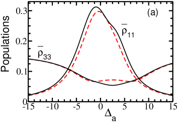
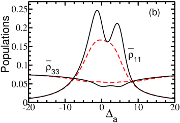
Figure 2: Steady state population of atomic levels as a function of the detuning $\Delta_{a}$ for the parameters $\gamma_{3}=1$, $W_{12}=5$, $\Delta_{b}=0$, $\Omega_{1}=\Omega_{2}=\Omega_{3}=3$, $\gamma_{1}=\gamma_{2}=0.5$ (a), $\gamma_{1}=\gamma_{2}=2$ (b). Actual values of $\overline{\rho}_{33}$ are three [six] times than shown in (a) [(b)]. The solid (dashed) curves are for $p=1$ $(p=0)$. The curves for $\overline{\rho}_{22}$ (not shown) have a similar behavior as that of $\overline{\rho}_{11}$.

To explore further the interference induced splittings of population resonances, we consider the case of near-degenerate excited levels $(W_{12}\ll\gamma_{1},\gamma_{2})$ and take the high intensity limit $(\Omega_{1},\Omega_{2},\Omega_{3}\gg W_{12},\gamma_{1},\gamma_{2},\gamma_{3})$ of applied lasers. For simplicity, we assume equal decay rates $\gamma_{1}=\gamma_{2}=\gamma$ for the upper transitions and examine two different cases, (a) $\gamma\gg\gamma_{3}$, (b) $\gamma=\gamma_{3}$, with respect to the decay rate of the lower transition. The numerical results are shown in Fig. 3 which are to be compared with Fig. 2. It is found that resonances in excited level populations occur at $\Delta_{a}=\pm\Omega$ [see Fig. 3(a)] in the limit $\Omega\gg\gamma\gg\gamma_{3}$, where $\Omega_{1}=\Omega_{2}=\Omega_{3}=\Omega$ is considered. In the case of equal decay rates $\gamma=\gamma_{3}$, analytical expressions for the population $(\rho_{11})$ can be obtained compactly in the presence $(p=1)$ and absence $(p=0)$ of interference as

$$\overline{\rho}_{11}(p=1) = \frac{\Omega^{4}\Delta_{a}^{6}+12\Omega^{6}\Delta_{a}^{4}+14\Omega^{8}\Delta_{a}^{2}+21\Omega^{10}}{2\Omega^{2}\Delta_{a}^{8}+16\Omega^{4}\Delta_{a}^{6}+52\Omega^{6}\Delta_{a}^{4}+2\Omega^{8}\Delta_{a}^{2}+84\Omega^{10}},$$

$$\overline{\rho}_{11}(p=0) = \frac{4\Omega^{4}\Delta_{a}^{6}+4\Omega^{8}\Delta_{a}^{4}+40\Omega^{10}\Delta_{a}^{2}+160\Omega^{10}}{8\Omega^{2}\Delta_{a}^{8}+8\Omega^{6}\Delta_{a}^{6}+64\Omega^{8}\Delta_{a}^{4}+240\Omega^{10}\Delta_{a}^{2}+960\Omega^{10}},$$ (18)

where all the parameters have been scaled in units of $\gamma$. These analytical formulas account well for the numerical results in Fig. 3(b). In order to understand physically the effect of interference, the atomic dynamics is further studied in the bases of symmetric and anti-symmetric states zhou2 defined by

$$|s\rangle = \frac{1}{\sqrt{\gamma_{1}+\gamma_{2}}}(\sqrt{\gamma_{1}}|1\rangle+\sqrt{\gamma_{2}}|2\rangle),$$

$$|a\rangle = \frac{1}{\sqrt{\gamma_{1}+\gamma_{2}}}(\sqrt{\gamma_{2}}|1\rangle-\sqrt{\gamma_{1}}|2\rangle).$$ (19)

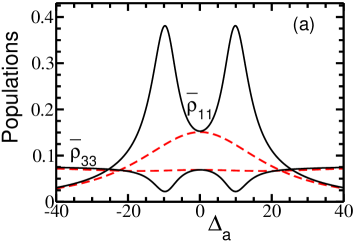
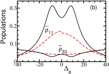
Figure 3: Steady state population of atomic levels as a function of the detuning $\Delta_{a}$ for the parameters $\gamma_{3}=1$, $W_{12}=0.2$, $\Delta_{b}=0$, $\Omega_{1}=\Omega_{2}=\Omega_{3}=10$, $\gamma_{1}=\gamma_{2}=5$ (a), $\gamma_{1}=\gamma_{2}=1$ (b). Actual values of $\overline{\rho}_{33}$ are six times than shown. The solid (dashed) curves are for $p=1$ $(p=0)$.

With $\gamma_{1}=\gamma_{2}=\gamma$ and using Eq. (19), the Hamiltonian Eq. (4) can be rewritten as

$$H_{I}= \hbar(\Delta_{a}-\frac{W_{12}}{2})(|s\rangle\langle s|+|a\rangle\langle a|)$$ (20)

$$+\frac{\hbar W_{12}}{2}(|s\rangle\langle a|+|a\rangle\langle s|)-\hbar\sqrt{2}\Omega(|s\rangle\langle 3|+|3\rangle\langle s|)$$

$$-\hbar\Omega(|3\rangle\langle 4|+|4\rangle\langle 3|).$$

From the above Hamiltonian, it is seen that only the symmetric state $|s\rangle$ is interacting with the light field. However, the antisymmetric state $|a\rangle$ may be populated by its coupling with the symmetric state because of the separation energy $(\hbar W_{12})$ between the excited atomic levels. This can become clear by analyzing the density matrix equations in the bases (19) :

$$\dot{\rho}_{aa} = \frac{iW_{12}}{2}\rho_{as}-\frac{iW_{12}}{2}\rho_{sa},$$

$$\dot{\rho}_{ss} = -4\gamma\rho_{ss}-\frac{iW_{12}}{2}\rho_{as}+\frac{iW_{12}}{2}\rho_{sa}$$ (21)

$$~{}~{}+i\sqrt{2}\Omega(\rho_{3s}-\rho_{s3}).$$

Here, the case of maximal quantum interference $(p=1)$ has been assumed. It is evident that the antisymmetric state is a non-decaying state for $p=1$ and it is coupled to the symmetric state for $W_{12}\neq 0$ (though small as in Fig. 3). In Fig. 4, the steady state populations of the symmetric and antisymmetric states are plotted for the same parameters of Fig. 3(a). The graphs show that the splitting of resonances occurs due to a high population of the antisymmetric state. We have so far assumed a fixed value for the lower transition detuning $(\Delta_{b}=0)$ and studied the dependence of populations on the upper transition detuning $(\Delta_{a})$. However, the results (not shown) will be qualitatively similar even in the general case of varying both $\Delta_{a}$ and $\Delta_{b}$.

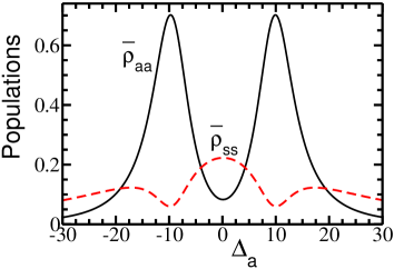
Figure 4: Steady state populations $\overline{\rho}_{aa}$ and $\overline{\rho}_{ss}$ as a function of the detuning $\Delta_{a}$ for the same parameters of Fig. 3(a) with $p=1$.

IV Resonance Fluorescence Spectrum

We now proceed to the study of the resonance fluorescence spectra of the driven atom. Since the atom is driven by two coherent fields, each field induces its own atomic dipole moment which then generates a scattered field. However, the fields scattered by the upper- and lower- transitions in the atom will have no correlations because the applied fields ($E_{a}$ ,$E_{b}$) are of quite different carrier frequencies ($\omega_{a}$, $\omega_{b}$). In the interaction picture, the negative- and positive-frequency parts of the polarization operators are written as

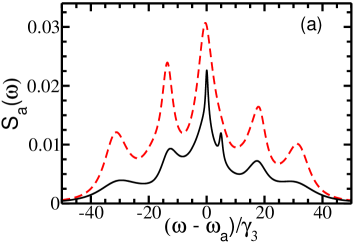
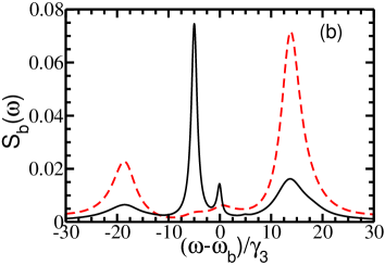
Figure 5: The incoherent spectrum of the fluorescent field generated by the dipoles (a) $\hat{\mathbf{P}}^{(+)}_{\omega_{a}}$ and (b) $\hat{\mathbf{P}}^{(+)}_{\omega_{b}}$ for the parameters $\gamma_{3}=1$, $W_{12}=10$, $\Delta_{a}=\Delta_{b}=0$, $\Omega_{1}=\Omega_{2}=10$, $\Omega_{3}=5$, $\gamma_{1}=\gamma_{2}=3$. The solid (dashed) curves are for $p=1$ $(p=0)$.

$$\hat{\mathbf{P}}^{(-)}_{\omega_{a}}(t) = \vec{\bm{\mu}}_{13}e^{i\omega_{a}t}|1\rangle\langle 3|+\vec{\bm{\mu}}_{23}e^{i\omega_{a}t}|2\rangle\langle 3|,$$

$$\hat{\mathbf{P}}^{(+)}_{\omega_{a}}(t) = [\hat{\mathbf{P}}^{(-)}_{\omega_{a}}(t)]^{\dagger},$$ (22)

$$\hat{\mathbf{P}}^{(-)}_{\omega_{b}}(t)=\vec{\bm{\mu}}_{34}e^{i\omega_{b}t}|3\rangle\langle 4|,~{}~{}~{}~{}~{}~{}\hat{\mathbf{P}}^{(+)}_{\omega_{b}}(t)=[\hat{\mathbf{P}}^{(-)}_{\omega_{b}}(t)]^{\dagger}.$$ (23)

To calculate the fluorescence spectra, we need the two-time expectation values of the polarization operator. The spectrum of resonance fluorescence is defined by the Fourier transformation of the two-time correlation or equivalently the real part of its Laplace transform:

$$S_{a}(\omega)=\hbox{Re}\int_{0}^{\infty}\lim_{t\rightarrow\infty}\langle\hat{\mathbf{P}}^{(-)}_{\omega_{a}}(t+\tau).\hat{\mathbf{P}}^{(+)}_{\omega_{a}}(t)\rangle e^{-i\omega\tau}d\tau,$$

$$S_{b}(\omega)=\hbox{Re}\int_{0}^{\infty}\lim_{t\rightarrow\infty}\langle\hat{\mathbf{P}}^{(-)}_{\omega_{b}}(t+\tau).\hat{\mathbf{P}}^{(+)}_{\omega_{b}}(t)\rangle e^{-i\omega\tau}d\tau.$$ (24)

Here, the index $a$ $(b)$ refers to the spectrum of the fluorescence light emitted by the atom with a central frequency $\omega_{a}$ $(\omega_{b})$. The Laplace transformation with variable $Z=i\omega$ of the correlation function, defined in the spectrum above, has a pole at $Z=i\omega_{a}$ $(Z=i\omega_{b})$ which attributes to the coherent Rayleigh scattering of the spectrum. The incoherent part is obtained by removing the contributions of the poles.

With the application of the quantum regression theorem fuli1 ; fuli2 ; narducci and using the steady state solutions Eq. (17) of the density matrix elements, the incoherent fluorescence spectra can be obtained as

$$S_{a}(\omega) = \hbox{Re}\Big{\{}{|\vec{\bm{\mu}}_{13}|}^{2}\big{[}\hat{M}_{11,9}\overline{\rho}_{14}+\hat{M}_{11,3}\overline{\rho}_{13}+\hat{M}_{11,12}\overline{\rho}_{12}$$

$$+\hat{M}_{11,11}\overline{\rho}_{11}+\sum_{j=1}^{15}\hat{N}_{11,j}\hat{I}_{j}\overline{\rho}_{13}\big{]}+\vec{\bm{\mu}}_{23}.\vec{\bm{\mu}}_{13}^{*}$$

$$\times\big{[}\hat{M}_{12,9}\overline{\rho}_{14}+\hat{M}_{12,3}\overline{\rho}_{13}+\hat{M}_{12,12}\overline{\rho}_{12}+\hat{M}_{12,11}$$

$$\times\overline{\rho}_{11}+\sum_{j=1}^{15}\hat{N}_{12,j}\hat{I}_{j}\overline{\rho}_{13}\big{]}+\vec{\bm{\mu}}_{13}.\vec{\bm{\mu}}_{23}^{*}\big{[}\hat{M}_{11,11}\overline{\rho}_{21}$$

$$+\hat{M}_{11,9}\overline{\rho}_{24}+\hat{M}_{11,3}\overline{\rho}_{23}+\hat{M}_{11,12}\overline{\rho}_{22}$$

$$+\sum_{j=1}^{15}\hat{N}_{11,j}\hat{I}_{j}\overline{\rho}_{23}\big{]}+{|\vec{\bm{\mu}}_{23}|}^{2}\big{[}\hat{M}_{12,11}\overline{\rho}_{21}+\hat{M}_{12,9}$$

$$\times\overline{\rho}_{24}+\hat{M}_{12,3}\overline{\rho}_{23}+\hat{M}_{12,12}\overline{\rho}_{22}+\sum_{j=1}^{15}\hat{N}_{12,j}\hat{I}_{j}$$

$$\times\overline{\rho}_{23}\big{]}\Big{\}},$$

where the matrices $\hat{M}={(Z-\hat{L})}^{-1}|_{Z=i(\omega-\omega_{a})}$ and $\hat{N}=\hat{L}^{-1}\hat{M}$. Similarly,

$$S_{b}(\omega)= \hbox{Re}\Big{\{}{|\vec{\bm{\mu}}_{34}|}^{2}\big{[}\hat{M}_{15,13}\overline{\rho}_{31}+\hat{M}_{15,14}\overline{\rho}_{32}+\hat{M}_{15,15}\overline{\rho}_{33}$$ (26)

$$+\sum_{j=1}^{15}\hat{N}_{15,j}\hat{I}_{j}\overline{\rho}_{34}\big{]}\Big{\}},$$

with the matrices $\hat{M}={(Z-\hat{L})}^{-1}|_{Z=i(\omega-\omega_{b})}$ and $\hat{N}=\hat{L}^{-1}\hat{M}$.

The set of equations (IV) and (26) can be used to obtain numerically the spectral characteristics of the driven atom. Figure 5 displays the numerical results by assuming equal decay rates $\gamma_{1}=\gamma_{2}$ of the upper atomic transitions. The spectra $S_{a}(\omega)$ and $S_{b}(\omega)$ are scaled in units of $|\vec{\bm{\mu}}_{13}|^{2}\gamma_{3}^{-1}$ and $|\vec{\bm{\mu}}_{34}|^{2}\gamma_{3}^{-1}$ respectively. In the presence of quantum interference $(p=1)$, the spectrum shows the typical line narrowing effect, as discussed in earlier publications zhou1 ; fuli1 ; fuli2 , in the fluorescent field with the central frequency $\omega_{a}$ [see Fig. 5(a)]. However, the spectral features get remarkably modified in the fluorescent field emitted by the lower atomic transitions. It is seen that the inner sideband in the fluorescence spectrum gets enhanced due to interference with a corresponding reduction in the intensity of the outer sidebands [compare solid and dashed curves in Fig. 5(b)]. A physical understanding of this interesting result can be obtained in the dressed state description of the atom-field interaction. The dressed states are defined as eigenstates of the time independent Hamiltonian (4) :

$$H_{I}|\Phi\rangle=\hbar\lambda|\Phi\rangle.$$ (27)

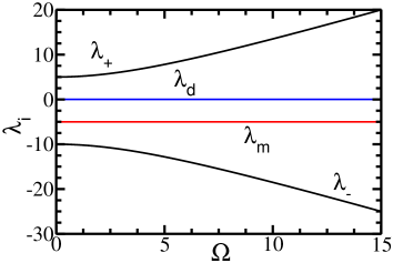
Figure 6: The dressed state eigenvalues versus the Rabi frequency $\Omega$ for the parameters $\gamma_{3}=1$, $W_{12}=10$, $\Delta_{a}=\Delta_{b}=0$, $\Omega_{3}=5$.

In the general parametric conditions, it is difficult to find analytical solutions to the eigenvalue equation (27). For simplicity, the case of two photon resonance $\Delta_{a}=\Delta_{b}=0$ is assumed in the following. In this case, there exists an eigenstate $|d\rangle$ with the eigenvalue $\lambda_{d}=0$ as

$$|d\rangle=\frac{1}{\sqrt{\Omega_{1}^{2}+\Omega_{3}^{2}}}[\Omega_{3}|1\rangle-\Omega_{1}|4\rangle].$$ (28)

The non-zero eigenvalues and the corresponding eigenstates can be obtained by diagonalizing the Hamiltonian $H_{I}$ in the basis of bare atomic states. We consider a special choice of parameters $\Omega_{1}=\Omega_{2}=\Omega$ and $\Omega_{3}=W_{12}/2$ [as in Fig. 5] which allows for simple analytical solutions. The operator $H_{I}$ has eigenstates $|m\rangle$, $|\pm\rangle$ with eigenvalues (in units of $\hbar$) $\lambda_{m}=-W_{12}/2$, $\lambda_{\pm}=(-W_{12}\pm\sqrt{W_{12}^{2}+32(\Omega^{2}+\frac{W_{12}^{2}}{4})})/4$, respectively, where

$$|m\rangle = \frac{1}{\sqrt{2(\Omega^{2}+(W_{12}^{2}/4))}}$$ (29)

$$\times\left[\Omega|1\rangle-\Omega|2\rangle+\frac{W_{12}}{2}|3\rangle+\frac{W_{12}}{2}|4\rangle\right],$$

$$|\pm\rangle = N_{\pm}\left[\Omega|1\rangle+\frac{\lambda_{\pm}\Omega}{(W_{12}+\lambda_{\pm})}|2\rangle-\lambda_{\pm}|3\rangle+\frac{W_{12}}{2}|4\rangle\right],$$

with $N_{\pm}=1\Big{/}\sqrt{\lambda_{\pm}^{2}[1+\Omega^{2}/{(W_{12}+\lambda_{\pm})}^{2}]+\Omega^{2}+W_{12}^{2}/4}$.

In order to interpret the numerical results in Fig. 5, we study the behavior of the dressed states in steady state with the inclusion of decay processes using Eq. (17). In Figs. 6 and 7, the dressed state eigenvalues $(\lambda\hbox{values})$ and its populations are shown as a function of the Rabi frequency $\Omega$ for the fixed value of $\Omega_{3}=W_{12}/2$. Note that the eigenvalues $\lambda_{d}$ and $\lambda_{m}$ are independent of the parameter $\Omega$. The peaks in the fluorescence spectrum can be attributed to transitions between the dressed states $|\Phi^{\prime}\rangle\leftrightarrow|\Phi\rangle$ $(\Phi,\Phi^{\prime}=d,m,+,-)$. For $p=0$ and $\Omega\gtrsim W_{12}$, the dressed states $|d\rangle$, $|+\rangle$, and $|-\rangle$ are well populated as shown in Fig. 7.

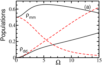
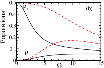
Figure 7: Steady state population of dressed states, (a) $\rho_{mm}$, $\rho_{dd}$ and (b) $\rho_{++}$, $\rho_{--}$, as a function of the Rabi frequency $\Omega$ for the parameters $\gamma_{3}=1$, $W_{12}=10$, $\Delta_{a}=\Delta_{b}=0$, $\Omega_{3}=5$, $\gamma_{1}=\gamma_{2}=3$. The solid (dashed) curves are for $p=1$ $(p=0)$.

The fluorescence peaks in Fig. 5 occur at the energy differences between these states. However, in the presence of interference $(p=1)$, the atomic population accumulates mostly in the dressed state $|m\rangle$ [see Fig. 7(a)]. This can be explained as due to a destructive quantum interference among the spontaneous decay pathways. The rate of transitions $|\Phi\rangle\rightarrow|\Phi^{\prime}\rangle$ between dressed states $|\Phi\rangle$ and $|\Phi^{\prime}\rangle$ is given by the squared dipole matrix elements which for the emission lines with the central frequencies $\omega_{a}$ and $\omega_{b}$ becomes

$$R_{\Phi,\Phi^{\prime}}^{a} = {|\langle\Phi^{\prime}|\hat{\mathbf{P}}^{(+)}_{\omega_{a}}|\Phi\rangle|}^{2}$$ (30)

$$= |\vec{\bm{\mu}}_{13}|^{2}[C_{1\Phi}^{2}+C_{2\Phi}^{2}+2pC_{1\Phi}C_{2\Phi}]C_{3\Phi^{\prime}}^{2},$$

$$R_{\Phi,\Phi^{\prime}}^{b} = {|\langle\Phi^{\prime}|\hat{\mathbf{P}}^{(+)}_{\omega_{b}}|\Phi\rangle|}^{2}$$ (31)

$$= |\vec{\bm{\mu}}_{34}|^{2}C_{3\Phi}^{2}C_{4\Phi^{\prime}}^{2},$$

where $|\vec{\bm{\mu}}_{13}|=|\vec{\bm{\mu}}_{23}|$ has been assumed and $C_{i\Phi}$’s $[i=1,2,3,4]$ denote the coefficients of the bare atomic states $|i\rangle$ in the dressed state $|\Phi\rangle$. As seen in the above Eq. (30), there is an interference term (p term) in the transition rate $R_{\Phi,\Phi^{\prime}}^{a}$ as a result of spontaneous decays along the $|1\rangle\rightarrow|3\rangle$ and $|2\rangle\rightarrow|3\rangle$ transitions. For the dressed state $|m\rangle$, this term cancels the square factors in the case of maximal interference $(p=1)$, thus suppressing the atomic decay, narrowing the spectral lines [shown in Fig. 5(a)] and enhancing the population [shown in Fig. 7(a)] in this state. However, the dressed state $|m\rangle$ can decay because of spontaneous emissions along the $|3\rangle\rightarrow|4\rangle$ transitions even when $p=1$ [see Eq. (31)]. This leads to the enhancement of the inner sideband in the spectrum [shown in Fig. 5(b)] of the fluorescence light emitted by the lower transitions in the atom. It is because only the states $|m\rangle$ and $|d\rangle$ are populated mainly in steady state. Finally, we note that the existence of atomic steady state and discussions so far assume the non-degenerate $(W_{12}\neq 0)$ case of excited atomic levels. In the degenerate case $(W_{12}=0)$, there exists no unique solution to Eq. (15) in steady state. In fact, the steady state fluorescence properties become dependent on the initial conditions due to degeneracy of the dressed states of the Hamiltonian.

V summary

We have investigated the resonance fluorescence from a driven Y-type atom when the presence of interference in spontaneous decay channels is important. At first, the steady state dynamics of the atom was studied using the density matrix approach. We have shown that the decay-induced interference can lead to splitting of resonances in the excited level populations calculated as a function of light detuning. This has been explained as due to high population of a non-decaying anti-symmetric state of the atom. Then, the role of interference in the spectral characteristics of the driven atom was examined. It is found that the interference results in narrowing of central peaks and enhancement of inner sidebands in the fluorescence spectrum. A physical understanding of the numerical results has been presented based on the dressed state theory of atom-field interaction. Clearly, the present work is open ended with the effects of interference in driven Y systems on two photon correlations and squeezing spectra remaining unexplored. Detailed investigations of such studies will be published elsewhere.

References

• (1) G. S. Agarwal, Quantum Optics, Springer Tracts in Modern Physics Vol. 70 (Springer-Verlag, Berlin, 1974).
• (2) S. Y. Zhu, R. C. F. Chan, and C. P. Lee, Phys. Rev. A 52, 710 (1995).
• (3) S. Y. Zhu and M. O. Scully, Phys. Rev. Lett. 76, 388 (1996); H. Huang, S. Y. Zhu, and M. S. Zubairy, Phys. Rev. A 55, 744 (1997); H. Lee, P. Polynkin, M. O. Scully, and S. Y. Zhu, ibid. 55, 4454 (1997).
• (4) E. Paspalakis and P. L. Knight, Phys. Rev. Lett. 81, 293 (1998).
• (5) E. Paspalakis, N. J. Kylstra, and P. L. Knight, Phys. Rev. Lett. 82, 2079 (1999).
• (6) D. A. Cardimona, M. G. Raymer, and C. R. Stroud, J. Phys. B 15, 65 (1982).
• (7) P. Zhou and S. Swain, Phys. Rev. Lett. 77, 3995 (1996); P. Zhou and S. Swain, Phys. Rev. A 56, 3011 (1997).
• (8) S. Swain, P. Zhou, and Z. Ficek, Phys. Rev. A 61, 043410 (2000); F. Carreño, M. A. Antón, and O. G. Calderón J. Opt. B: Quantum Semiclassical Opt. 6, 315 (2004).
• (9) S. Y. Gao, F. L. Li, and S. Y. Zhu, Phys. Rev. A 66, 043806 (2002).
• (10) M. Macovei, J. Evers, and C. H. Keitel, Phys. Rev. Lett. 91, 233601 (2003).
• (11) A. K. Patnaik and G. S. Agarwal, Phys. Rev. A 59, 3015 (1999); P. Zhou and S. Swain, Opt. Commun. 179, 267 (2000).
• (12) A. K. Patnaik and G. S. Agarwal, J. Mod. Opt. 45, 2131 (1998).
• (13) Z. Ficek and S. Swain, Phys. Rev. A 69, 023401 (2004).
• (14) F. L. Li and S. Y. Zhu, Phys. Rev. A 59, 2330 (1999); F. L. Li, S. Y. Gao, and S. Y. Zhu, ibid. 67, 063818 (2003).
• (15) F. L. Li, S. Y. Zhu, and A. Q. Ma, J. Mod. Opt. 48, 439 (2001).
• (16) M. A. Antón, O. G. Calderón, and F. Carreño, Phys. Rev. A 72, 023809 (2005).
• (17) B. P. Hou, S. J. Wang, W. L. Yu, and W. L. Sun, Phys. Rev. A 69, 053805 (2004); G. S. Agarwal and W. Harshawardhan, Phys. Rev. Lett. 77, 1039 (1996).
• (18) An experimental arrangement of this atomic model is given in [J. Y. Gao, S. H. Yang, D. Wang, X. Z. Guo, K. X. Chen, Y. Jiang, and B. Zhao, Phys. Rev. A 61, 023401 (2000)].
• (19) This result is very similar to that of a driven three-level atom in the ladder configuration reported by Z. Ficek, B. J. Dalton, and P. L. Knight [Phys. Rev. A 51, 4062 (1995)].
• (20) A.S. Manka et al. 43, 3748 (1991).