Heavy-light decay constant at the $1/m$ order of HQET

Abstract:

Following the strategy developed by the ALPHA collaboration, we present a method to compute non-perturbatively the decay constant of a heavy-light meson in HQET including the 1/m corrections. We start by a matching between HQET and QCD in a small volume to determine the parameters of the effective theory non-perturbatively. Observables in the effective theory are then evolved to larger volumes. In two steps a large enough volume is reached to determine the physical decay constant. Some preliminary results in the quenched approximation are shown.

1 Introduction

A few years ago, a non-perturbative formulation of Heavy Quark Effective Theory (HQET) has been given in [1] - see [2] for a review given at this conference. In particular the problem of power divergences is solved through a finite volume matching. Last year, this has been applied to the quenched computation of the b-quark mass at the $1/m$ order [3]. In the same spirit, we present here a strategy to compute a heavy-light decay constant. We start by writing the Lagrangian at the leading order (i.e. in the static approximation) and add a kinetic and a magnetic piece (we follow the conventions of [3] and set the counterterm $\delta_{m}$ to zero)

$${\mathcal{L}}_{\rm{HQET}}=\overline{\psi}_{\rm h}\,D_{0}\,\psi_{\rm h}-\omega_{\mathrm{kin}}\overline{\psi}_{\rm h}{\bf D}^{2}\psi_{\rm h}\,-\omega_{\mathrm{spin}}\overline{\psi}_{\rm h}{\boldsymbol{\sigma}}\!\cdot\!{\bf B}\psi_{\rm h}\;.$$ (1)

A precise definition of the operators $D_{0}$, ${\bf D}^{2}$ and ${\boldsymbol{\sigma}}\!\cdot\!{\bf B}$ can be found in [3]. Here we just note that $\omega_{\mathrm{kin}}$ and $\omega_{\mathrm{spin}}$ are some bare parameters of the effective theory.

1.1 Schrödinger functional (SF) correlation functions

In QCD, we consider the (renormalized and improved) current to boundary correlators $f_{\rm A}$ and $k_{V}$ defined - up to improvement factors such as $(1+b_{\rm A}am_{\rm q,b})$ - in the SF by

$$f_{\rm A}(x_{0}) = -Z_{A}\,Z_{\zeta}^{2}\,{a^{6}\over 2}\,\sum_{{\bf y},{\bf z}}\langle\left(A_{\rm I}\right)_{0}(x)\,\bar{\zeta}_{\rm b}({\bf y})\gamma_{5}\zeta_{\rm l}({\bf z})\rangle,$$ (2)

$$k_{\rm V}(x_{0}) = -Z_{V}\,Z_{\zeta}^{2}\,{a^{6}\over 6}\sum_{{\bf y},{\bf z},k}\langle\left(V_{\rm I}\right)_{k}(x)\,\bar{\zeta}_{\rm b}({\bf y})\gamma_{k}\zeta_{\rm l}({\bf z})\rangle,$$ (3)

where the improved currents $A_{\rm I}(x)$ and $V_{\rm I}(x)$ are defined as in [1].
We also consider the boundary to boundary correlators

$$f_{1} = -Z_{\zeta}^{4}\,{a^{12}\over 2L^{6}}\,\sum_{{\bf u},{\bf v},{\bf y},{\bf z}}\langle\bar{\zeta}_{\rm l}^{\prime}({\bf u})\gamma_{5}\zeta_{\rm b}^{\prime}({\bf v})\,\bar{\zeta}_{\rm b}({\bf y})\gamma_{5}\zeta_{\rm l}({\bf z})\rangle,$$ (4)

$$k_{1} = -Z_{\zeta}^{4}\,{a^{12}\over 6L^{6}}\,\sum_{{\bf u},{\bf v},{\bf y},{\bf z},k}\langle\bar{\zeta}_{\rm l}^{\prime}({\bf u})\gamma_{k}\zeta_{\rm b}^{\prime}({\bf v})\,\bar{\zeta}_{\rm b}({\bf y})\gamma_{k}\zeta_{\rm l}({\bf z})\rangle.$$ (5)

Expanding these correlators at the $1/m$ order of HQET, and using spin-flavor symmetry, one finds 

$$f_{\rm A}(x_{0}) = Z_{\rm A}^{\rm HQET}Z_{\zeta_{\mathrm{h}}}Z_{\zeta}{\rm e}^{-m_{\rm bare}x_{0}}\left\{f_{\rm A}^{\rm stat}(x_{0})+c_{\rm A}^{\rm HQET}f_{\delta\rm A}^{\rm stat}(x_{0})+\omega_{\mathrm{kin}}f_{\rm A}^{\rm kin}(x_{0})+\omega_{\mathrm{spin}}f_{\rm A}^{\rm spin}(x_{0})\right\}\,,$$

$$k_{\rm V}(x_{0}) = -Z_{\rm V}^{\rm HQET}Z_{\zeta_{\mathrm{h}}}Z_{\zeta}{\rm e}^{-m_{\rm bare}x_{0}}\left\{f_{\rm A}^{\rm stat}(x_{0})+c_{\rm V}^{\rm HQET}f_{\delta\rm A}^{\rm stat}(x_{0})+\omega_{\mathrm{kin}}f_{\rm A}^{\rm kin}(x_{0})-\frac{1}{3}\omega_{\mathrm{spin}}f_{\rm A}^{\rm spin}(x_{0})\right\}\,,$$

$$f_{1} = Z_{\zeta_{\mathrm{h}}}^{2}Z_{\zeta}^{2}{\rm e}^{-m_{\rm bare}T}\left\{f_{1}^{\rm stat}+\omega_{\mathrm{kin}}f_{1}^{\rm kin}+\omega_{\mathrm{spin}}f_{1}^{\rm spin}\right\}\,,$$

$$k_{1} = Z_{\zeta_{\mathrm{h}}}^{2}Z_{\zeta}^{2}{\rm e}^{-m_{\rm bare}T}\left\{f_{1}^{\rm stat}+\omega_{\mathrm{kin}}f_{1}^{\rm kin}-\frac{1}{3}\omega_{\mathrm{spin}}f_{1}^{\rm spin}\right\}\,,$$

where $m_{\rm bare}$ is the (linearly divergent) bare quark mass.

1.2 Basic observable

We consider a volume $L^{3}$ with a time extent $T=L$, and define (in QCD)

$$\Phi_{\rm F}^{\rm QCD}(L)=\ln\left({{-f_{\rm A}(L/2)}\over{\sqrt{f_{1}}}}\right)$$

In the large volume limit, this observable is related to the decay constant, $F_{\rm B}$, by

$$\Phi_{\rm F}^{\rm QCD}(L)\stackrel{{\scriptstyle L\gg 1/\Lambda}}{{\longrightarrow}}\ln\left(\frac{1}{2}F_{\rm B}\sqrt{m_{\rm B}L^{3}}\right).$$ (6)

In a small volume  of space extent $L_{1}\simeq 0.4\,{\rm fm}$, this observable is matched to its HQET expression

$$\Phi_{\rm F}^{\rm QCD}(L_{1})=\Phi_{\rm F}^{\rm HQET}(L_{1})\;.$$ (7)

Using the expansions of the correlators $f_{\rm A}$ and $f_{1}$ given previously, one finds for the rhs at the static and at the $1/m$ order

$$\Phi_{\rm F}^{\rm stat}(L) = \ln Z_{\rm A}^{\rm stat}+{\ln\left({-f_{\rm A}^{\rm stat}(L/2)\over\sqrt{f_{1}^{\rm stat}}}\right)}+{\rm O}(1/m),$$ (8)

$$\Phi_{\rm F}^{\rm stat}(L)+\Phi_{\rm F}^{1/m}(L) = \ln Z_{\rm A}^{\rm HQET}+\ln\left({-f_{\rm A}^{\rm stat}(L/2)\over\sqrt{f_{1}^{\rm stat}}}\right)+c_{\rm A}^{\rm HQET}{f_{\delta\rm A}^{\rm stat}(L/2)\over f_{\rm A}^{\rm stat}(L/2)}$$

$$+\omega_{\mathrm{kin}}\left({f_{\rm A}^{\rm kin}(L/2)\over f_{\rm A}^{\rm stat}(L/2)}-{f_{1}^{\rm kin}\over f_{1}^{\rm stat}}\right)+\omega_{\mathrm{spin}}\left({f_{\rm A}^{\rm spin}(L/2)\over f_{\rm A}^{\rm stat}(L/2)}-{f_{1}^{\rm spin}\over f_{1}^{\rm stat}}\right)+{\rm O}(1/m^{2}).$$

1.3 Evolution to larger volumes, in the static approximation

In order to clarify the discussion, we first explain the strategy in the static approximation, the generalization to the $1/m$ order will be done in the next section. We start by the matching of HQET to QCD in the volume $L_{1}$, at the static order : $\Phi_{\rm F}^{\rm QCD}(L_{1})=\Phi_{\rm F}^{\rm stat}(L_{1}).$ The evolution to a volume $L_{\infty}=L_{3}=2L_{2}=4L_{1}$ is then done, within the effective theory, in the following way:

$$\Phi_{\rm F}(L_{\infty})=[\Phi_{\rm F}^{\rm stat}(L_{\infty})-\Phi_{\rm F}^{\rm stat}(L_{2})]+[\Phi_{\rm F}^{\rm stat}(L_{2})-\Phi_{\rm F}^{\rm stat}(L_{1})]+\Phi_{\rm F}^{\rm QCD}(L_{1})\;.$$ (10)

We note that $Z_{\rm A}^{\rm stat}$ cancels in the differences $[\Phi_{\rm F}^{\rm stat}(2L)-\Phi_{\rm F}^{\rm stat}(L)]$. Using the renormalized SF coupling $\bar{g}^{2}(L)$ [4], we define the static step scaling function (ssf)

$$\sigma_{\rm F}^{\rm stat}(u) = \left[\Phi_{\rm F}^{\rm stat}(2L)-\Phi_{\rm F}^{\rm stat}(L)\right]_{\bar{g}^{2}(L)=u}=\lim_{a/L\to 0}\Sigma_{\rm F}^{\rm stat}(u,a/L)$$ (11)

$$\Sigma_{\rm F}^{\rm stat}(u,a/L) = \left[\zeta^{\rm stat}(2L)-\zeta^{\rm stat}(L)\right]_{\bar{g}^{2}(L)=u}\;\mbox{ where }\zeta^{\rm stat}(L)=\ln\left({-f_{\rm A}^{\rm stat}(L/2)\over\sqrt{f_{1}^{\rm stat}}}\right)\;.$$ (12)

We can now rewrite the rhs of eq (10) as the sum of three continuum terms

$$\Phi_{\rm F}(L_{\infty})=\sigma_{\rm F}^{\rm stat}(u_{2})+\sigma_{\rm F}^{\rm stat}(u_{1})+\Phi_{\rm F}^{\rm QCD}(L_{1})\,,\mbox{ where }u_{\rm k}=\bar{g}^{2}(L_{\rm k})\;.$$ (13)

Before discussing the $1/m$ corrections we close this section by a few remarks :

• The different terms in the eq (12) have to be computed at the same value of the lattice spacing (in order to insure that $\Sigma_{F}$ has a well defined continuum limit). This is due to divergences proportional to the logarithm of the lattice spacing that one has to cancel.

• In eq. (13), the entire quark mass dependence comes from $\Phi_{\rm F}^{\rm QCD}(L_{1})$.

• At this order, since there is only one matching constant to eliminate ($Z_{\rm A}^{\rm stat}$), it is sufficient to match one observable ($\Phi_{\rm F}$).

1.4 Including $1/m$ corrections

At this order, there are three more matching parameters in $\Phi_{\rm F}$ compared to the static case . Therefore, to determine them, we introduce three other observables defined in a volume of space extent $L$ and we give their expressions at the $1/m$ order

$$\Phi_{1}(L) \equiv \frac{1}{4}(R_{1}^{\rm P}+3R_{1}^{\rm V})-R_{1}^{\rm stat}=\omega_{\mathrm{kin}}R_{1}^{\rm kin}\;,$$ (14)

$$\Phi_{2}(L) \equiv {{3}\over{4}}\ln\left({{f_{1}}\over{k_{1}}}\right)=\omega_{\mathrm{spin}}{{f_{1}^{\rm spin}}\over{f_{1}^{\rm stat}}}\qquad\mbox{with }T=L/2\;,$$ (15)

$$\Phi_{3}(L) \equiv R_{\rm A}(L/2)-R_{\rm A}^{\rm stat}(L/2)=c_{\rm A}^{\rm HQET}R_{\delta{\rm A}}(L/2)+\omega_{\mathrm{kin}}R_{\rm A}^{\rm kin}(L/2)+\omega_{\rm spin}R_{\rm A}^{\rm spin}(L/2)\;,\;$$ (16)

where the definitions of the ratios $R$ can be found in [3] . Together with $\Phi_{\rm F}$, given at this order by (1.2), we then have a set of four observables. In these observables, we have chosen to subtract the static part (when existing) from the QCD one, as we did in the mentioned reference. This is perfectly legitimate because they both have a continuum limit, and this simplifies the equations.
Like in the static case, the matching is imposed in the volume $L_{1}$. This allows us to replace in (1.2) the parameters $\omega_{\mathrm{kin}}$, $\omega_{\mathrm{spin}}$ and $c_{\rm A}^{\rm HQET}$ by a combination of QCD and HQET quantities.
The evolution to the volume $L_{2}$ is given by

$$\Phi_{\rm F}(L_{2}) = \Phi_{\rm F}^{\rm HQET}(L_{2})-\Phi_{\rm F}^{\rm HQET}(L_{1})+\Phi_{\rm F}^{\rm QCD}(L_{1})$$ (17)

$$= \left[\Phi_{\rm F}^{\rm stat}(L_{2})-\Phi_{\rm F}^{\rm stat}(L_{1})\right]+\left[\Phi_{\rm F}^{1/m}(L_{2})-\Phi_{\rm F}^{1/m}(L_{1})\right]+\Phi_{\rm F}^{\rm QCD}(L_{1})\;.$$ (18)

The ssf for the static term has already been given in the previous part, and for the $1/m$ part we write

$$\Phi_{\rm F}^{1/m}(2L)-\Phi_{\rm F}^{1/m}(L)=\sum_{\rm i}\sigma_{\rm i}(\bar{g}^{2}(L))\Phi_{\rm i}(L)\;.$$ (19)

The expressions for the ssf can be found from the last equation by using (1.2) together with (14), (15), (16) in the volume $L_{1}$. The explicit definitions are given in the appendix.
In the step $L_{2}\rightarrow L_{\infty}$, we need $\Phi_{\rm i}(L_{2},M)$, and we are then lead to define the ssf for the $\Phi_{\rm i}$ :

$$\Phi_{\rm i}(L_{2})=\sum_{j}\sigma_{\rm ij}(\bar{g}^{2}(L))\Phi_{\rm j}(L_{1})\,.$$ (20)

We can write down the final equation for $\Phi_{\rm F}$

$$\Phi_{\rm F}(L_{\infty})=\sigma_{\rm F}^{\rm stat}(u_{2})+\sigma_{\rm F}^{\rm stat}(u_{1})+\sum_{\rm ij}\sigma_{\rm i}(u_{2})\sigma_{\rm ij}(u_{1})\Phi_{\rm j}(L_{1})+\sum_{\rm i}\sigma_{\rm i}(u_{1})\Phi_{\rm i}(L_{1})+\Phi_{\rm F}^{\rm QCD}(L_{1})$$ (21)

2 Results in the quenched approximation

We used basically the same data as in [3], in which the reader can find the details of the simulation. The simulations are done with non-perturbatively $\rm O(a)$-improved Wilson fermions. The light quark mass is fixed to the strange one. Concerning HQET, we used the HYP actions [5], which help to have a reasonable statistical precision. We show the continuum extrapolations in fig. 1.

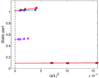
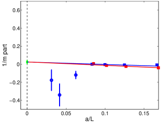
Figure 1: Continuum extrapolations of the various terms appearing in eq. (21). The QCD contribution $\Phi_{\rm F}^{\rm QCD}$ (diamonds) and the static part are shown on the left (the circles represent the large volume contribution $\sigma_{\rm F}^{\rm stat}(u_{2})$, and the squares the small volume part $\sigma_{\rm F}^{\rm stat}(u_{1})$ ). The $1/m$ correction is plotted on the right, the circles represent the large volume terms $\sum_{\rm ij}\sigma_{\rm i}(u_{2})\sigma_{\rm ij}(u_{1})\Phi_{\rm j}(L_{1})$, and the squares the small volume part $\sum_{\rm i}\sigma_{\rm i}(u_{1})\Phi_{\rm i}(L_{1})$. The color blue stands for HYP2, and red for HYP1 [5].

The extrapolations are done linearly in $(a/L)^{2}$ for QCD as well as for the static part, but in $a/L$ for the $1/m$ term, because of the absence of $\rm O(a)$ improvement. The ordinate scale is the same in order to compare the relative size of the different contributions. Concerning the precision, one can see that the total error is largely dominated by the one of the $1/m$ part in the large volume. Since for this part the results are not yet completely satisfactory, we refrain from performing a continuum extrapolation. We will use the result at the finest lattice spacing only ($\beta\sim 6.45,\,L/a=32$).
Our preliminary results for $F_{B_{s}}$ are shown in table 1. In the first column we give the results in the static approximation, while in the other columns, we have included the $1/m$ corrections. We observe that in the static approximation, depending on the matching condition represented here by $\theta$  , the result can change by $7\%$. This variation disappears when the $1/m$ terms are included. Note that differences of $F_{\rm B_{\rm s}}^{\rm stat+1/m}$, table 1, have much smaller error than their individual values, for example

$$F_{\rm B_{\rm s}}^{\rm stat+1/m}(\theta_{0}=0,\theta_{1}=1,\theta_{2}=0)-F_{\rm B_{\rm s}}^{\rm stat+1/m}(\theta_{0}=1,\theta_{1}=0,\theta_{2}=0.5)=4\pm 2\mbox{ MeV}.$$ (22)

The other information is that the $1/m$ term contributes (with a minus sign) up to $\sim 15\%$ to the final result. One can see that adding the $1/m$ terms increases the size of the statistical errors, as expected from the previous plots. This is due to the fact that the signal for the $1/m$ part in large volume is more difficult to extract than in the static case, and also because of the absence of $\rm O(a)$-improvement at this order. We also note that our result is compatible with a recent computation done with a different method, but which also goes beyond the leading order of HQET [6].

	$F_{\rm B_{s}}^{\rm stat}$	$F_{\rm B_{s}}^{\rm stat+1/m}$
$\theta_{0}$		$\theta_{1}=0$	$\theta_{1}=0.5$	$\theta_{1}=1$
		$\theta_{2}=0.5$	$\theta_{2}=1$	$\theta_{2}=0$
$0$	$224\pm 3$	$185\pm 21$	$186\pm 22$	$189\pm 22$
$0.5$	$220\pm 3$	$185\pm 21$	$187\pm 22$	$189\pm 22$
$1$	$209\pm 3$	$184\pm 21$	$185\pm 21$	$188\pm 22$

Table 1: Results for $F_{B_{s}}$ in MeV with and without the $1/m$ corrections, for different values of the $\theta$ angles.

3 Conclusion

We have shown how to perform a non-perturbative computation of a heavy-light decay constant at $1/m$ order of HQET, and we have given preliminary numerical results in the quenched approximation. The inclusion of the dynamical quarks is on the way [7, 8]. Applying this method for $N_{f}>0$ should allow for precise computations of the heavy-light decay constant, with a good control on the systematic errors. Note in particular that eq. (22) is a good sign of the absence of significant $1/m^{2}$ corrections. On the numerical side, the cancellations of the divergences require sufficient statistical precision, and we hope that the all-to-all propagator, like proposed in [9, 10] will be of great help there.

Acknowledments
We thank NIC for allocating computer time on the APE computers to this project and the APE group at Zeuthen for its support.

4 Appendix: The step scaling functions

In order to have more compact notations, we replace $\Phi_{\rm F}$ by $\Phi_{4}$, such that the ssf $\sigma_{\rm i}$ introduced in eq. (19) are now represented by $\sigma_{\rm 4i}\,$. We can rewrite eq. (19) together with eq.( 20) as

$$\Phi_{\rm i}(L_{\rm k+1},M)=\sum_{j=1}^{4}\sigma_{\rm ij}(u_{\rm k})\Phi_{\rm j}(L_{\rm k},M)+\delta_{\rm 4i}\sigma_{\zeta}(u_{\rm k})\,.$$ (23)

The ssf are then given by a four by four matrix

σ31σ32σ330σ41σ42σ431)delimited-[]subscript𝜎ijfragments fragments fragmentsσ31fragmentsσ32fragmentsσ330fragmentsσ41fragmentsσ42fragmentsσ431\left[\sigma_{\rm ij}\right]=\left(\begin{tabular}[]{cccc}$\sigma_{11}$&0&0&0\\ 0&$\sigma_{22}$&0&0\\ $\sigma_{31}$&$\sigma_{32}$&$\sigma_{33}$&0\\ $\sigma_{41}$&$\sigma_{42}$&$\sigma_{43}$&1\\ \end{tabular}\right)

σ110000σ2200σ110000σ2200

To give their explicit expressions, we define

$$\Psi^{\rm kin}(L)=\left({f_{\rm A}^{\rm kin}(T/2)\over f_{\rm A}^{\rm stat}(T/2)}-{f_{1}^{\rm kin}\over f_{1}^{\rm stat}}\right)\;,\quad\Psi^{\rm spin}(L)=\left({f_{\rm A}^{\rm spin}(T/2)\over f_{\rm A}^{\rm stat}(T/2)}-{f_{1}^{\rm spin}\over f_{1}^{\rm stat}}\right)\quad\mbox{and}\quad\rho_{\delta_{\rm A}}(L)={f_{\delta\rm A}^{\rm stat}(T/2)\over f_{\rm A}^{\rm stat}(T/2)}\;.$$

Then, one finds:

$$\Sigma_{11}(u) = \left[R_{1}^{\rm kin}(2L)/R_{1}^{\rm kin}(L)\right]_{\bar{g}^{2}(L)=u}\;,\qquad\Sigma_{22}(u)=\left[\rho_{1}^{\rm spin}(2L)/\rho_{1}^{\rm spin}(L)\right]_{\bar{g}^{2}(L)=u}\;,$$

$$\Sigma_{31}(u) = \left[{1\over R_{1}^{\rm kin}(L)}\left(R_{\rm A}^{\rm kin}(2L)-{R_{\rm A}^{\rm kin}(L)\,R_{\delta_{\rm A}}(2L)\over R_{\delta_{\rm A}}(L)}\right)\right]_{\bar{g}^{2}(L)=u}\;,$$

$$\Sigma_{32}(u) = \left[{1\over\rho_{1}^{\rm spin}(L)}\left(R_{\rm A}^{\rm spin}(2L)-{R_{\rm A}^{\rm spin}(L)R_{\delta_{\rm A}}(2L)\over R_{\delta_{\rm A}}(L)}\right)\right]_{\bar{g}^{2}(L)=u}\;,\qquad\Sigma_{33}(u)=\left[{R_{\delta_{\rm A}}(2L)\over R_{\delta_{\rm A}}(L)}\right]_{\bar{g}^{2}(L)=u}\;,$$

$$\Sigma_{41}(u) = \left[{1\over R_{1}^{\rm kin}(L)}\left(\Psi^{\rm kin}(2L)-\Psi^{\rm kin}(L)-{\rho_{\delta_{\rm A}}(2L)-\rho_{\delta_{\rm A}}(L)\over R_{\delta_{\rm A}}(L)}\,R_{\rm A}^{\rm kin}(L)\right)\right]_{\bar{g}^{2}(L)=u}\;,$$

$$\Sigma_{42}(u) = \left[{1\over\rho_{1}^{\rm spin}(L)}\left(\Psi^{\rm spin}(2L)-\Psi^{\rm spin}(L)-{\rho_{\delta_{\rm A}}(2L)-\rho_{\delta_{\rm A}}(L)\over R_{\delta_{\rm A}}(L)}\,R_{\rm A}^{\rm spin}(L)\right)\right]_{\bar{g}^{2}(L)=u}\;,$$

$$\Sigma_{43}(u) = \left[{\rho_{\delta_{\rm A}}(2L)-\rho_{\delta_{\rm A}}(L)\over R_{\delta_{\rm A}}(L)}\right]_{\bar{g}^{2}(L)=u}\;.$$

References

- [1] ALPHA Collaboration, J. Heitger and R. Sommer, Non-perturbative heavy quark effective theory, JHEP 02 (2004) 022 [hep-lat/0310035].
- [2] M. Della Morte, Standard model parameters and heavy quarks on the lattice, PoS LAT2007 008.
- [3] M. Della Morte, N. Garron, M. Papinutto, and R. Sommer, Heavy quark effective theory computation of the mass of the bottom quark, JHEP 01 (2007) 007 [hep-ph/0609294].
- [4] ALPHA Collaboration, S. Capitani, M. Lüscher, R. Sommer, and H. Wittig, Non-perturbative quark mass renormalization in quenched lattice QCD, Nucl. Phys. B544 (1999) 669 [hep-lat/9810063].
- [5] M. Della Morte, A. Shindler, and R. Sommer, On lattice actions for static quarks, JHEP 08 (2005) 051 [hep-lat/0506008].
- [6] D. Guazzini, R. Sommer, and N. Tantalo, and from a combination of HQET and QCD, PoS LAT2006 (2006) 084 [hep-lat/0609065].
- [7] M. Della Morte, P. Fritzsch, J. Heitger, H. Meyer, H. Simma, and R. Sommer, Towards a non-perturbative matching of HQET and QCD with dynamical light quarks, PoS LAT2007 246.
- [8] M. Della Morte, P. Fritzsch, B. Leder, H. Meyer, H. Simma, R. Sommer, S. Takeda, O. Witzel, and U. Wolff, Preparing for simulations at small lattice spacings, PoS LAT2007 255.
- [9] J. Foley et. al., Practical all-to-all propagators for lattice QCD, Comput. Phys. Commun. 172 (2005) 145 [hep-lat/0505023].
- [10] M. Lüscher, Local coherence and deflation of the low quark modes in lattice QCD, JHEP 07 (2007) 081 [hep-lat/07062298].