Classical and quantum behavior of dynamical systems defined by functions of solvable Hamiltonians

Abstract

We discuss the classical and quantum mechanical evolution of systems described by a Hamiltonian that is a function of a solvable one, both classically and quantum mechanically. The case in which the solvable Hamiltonian corresponds to the harmonic oscillator is emphasized. We show that, in spite of the similarities at the classical level, the quantum evolution is very different. In particular, this difference is important in constructing coherent states, which is impossible in most cases. The class of Hamiltonians we consider is interesting due to its pedagogical value and its applicability to some open research problems in quantum optics and quantum gravity.

I Introduction

The goal of this article is to discuss the classical and quantum mechanics of systems whose Hamiltonian $H=f(H_{0})$ is a function of the harmonic oscillator Hamiltonian $H_{0}$. The results can be easily generalized to other choices of $H_{0}$ for which the classical and quantum equations of motion are exactly solvable.

Once we solve the classical equations of motion for $H_{0}$, it is possible to study a system described by $H=f(H_{0})$. Although the solution is a straightforward exercise in classical mechanics, we will discuss it in detail because it is interesting to compare the solutions corresponding to both classical and quantum dynamics. Quantum mechanically the unitary evolution operator for $\hat{H}=f(\hat{H_{0}})$ can also be constructed exactly once we know the evolution generated by $\hat{H}_{0}$. A comparison of the dynamics given by $\hat{H}_{0}$ and $f(\hat{H}_{0})$ will allow us to analyze some distinctive features of the coherent states of the harmonic oscillator and discuss the difficulties that appear when we try to construct similar states for the dynamics generated by $f(\hat{H_{0}})$. This comparison will help us understand some aspects of the open problem of building appropriate semiclassical states for general Hamiltonians.

Non-trivial systems whose evolution can be solved exactly both classically and quantum mechanically are rare. Usually, realistic systems are described by Hamiltonians of the form $H=H_{0}+H_{1}$, where $H_{0}$ is a solvable Hamiltonian and $H_{1}$ represents a perturbation. In most cases it is impossible to give the solutions to the equations defined $H$, so it is necessary to resort to approximation methods. The starting point of perturbation theory is the known dynamics generated by $H_{0}$. The simplest choice of $H_{0}$ is the Hamiltonian of a free particle. However, if we are considering a system that has bound states, it is much better to consider a solvable $H_{0}$ with bound states, such as the harmonic oscillator.

In this paper we consider a different way to perturb a solvable Hamiltonian $H_{0}$ by considering a function of it. If this function is close to the identity, it will be possible to treat the system as a perturbation of $H_{0}$ in the usual sense; otherwise it will provide different but still solvable dynamics.

We point out that these kind of Hamiltonians appear in some physical applications, for example, in the context of quantum optics and classical and quantum gravity. For instance, the propagation of light in Kerr mediabanerji ; leonski — media with a refractive index with a component that depends on the intensity of the propagating electric field — is described (for a single mode field given by the creation and annihilation operators $\hat{a}^{\dagger}$ and $\hat{a}$ and in the low loss approximation) by

$$\hat{H}=\chi(\hat{N}^{2}-\hat{N})=\chi\mbox{:$\hat{N}^{2}$:}=\chi\,\hat{a}^{\dagger 2}\hat{a}^{2},$$ (1)

where $\chi$ is related to the susceptibility of the medium, and the Hamiltonian is a function of the number operator $\hat{N}=\hat{a}^{\dagger}\hat{a}$. The symbol $:\,\,:$ denotes normal ordering (creation operators to the left of the annihilation ones) and the operators $\hat{a}$ and $\hat{a}^{\dagger}$ satisfy the usual commutation relation $[\hat{a},\hat{a}^{\dagger}]=1$.

Another situation where we find this kind of Hamiltonian is in general relativity. Einstein-RosenEinstein waves are cylindrically symmetric solutions to the Einstein equations in vacuum. The Hamiltonian that describes this system isAshtekar2 ; Fernando

$$H=2(1-\exp(-H_{0}/2)),$$ (2)

where $H_{0}$ is a free (and easily solvable) Hamiltonian.

The examples we have mentioned are field theories with Hamiltonians $f(H_{0})$ that are functions of free Hamiltonians $H_{0}$ (i.e. quadratic in the fields and their canonical conjugate momenta) describing an infinite number of harmonic oscillators. Although these models can be solved, we will concentrate here on finite dimensional examples to avoid field theoretical complications, in particular, issues related to the presence of an infinite number of degrees of freedom and the coupling of the infinite different modes induced by the function $f$.

We consider

$$H=f(H_{0}),\qquad H_{0}=\frac{p^{2}}{2m}+\frac{k}{2}x^{2}.$$ (3)

To simplify the calculations, we will assume that $m=1$ and $k=1$. We will also work with an arbitrary function $f$ (subject to some mild smoothness conditions) until the very end of our discussion. At that point we will make some explicit calculations by using the functional form of the Einstein-Rosen Hamiltonian. We emphasize that similar arguments could be made for any system whose Hamiltonian is a function of a solvable one.

II Classical treatment

We first discuss the classical solution for $H_{0}=\frac{1}{2}(p_{0}^{2}+x_{0}^{2})$. The dynamics generated by $H_{0}$ is given by the equations

$$\frac{dx_{0}}{dT}=p_{0},\qquad\frac{dp_{0}}{dT}=-x_{0}.$$ (4)

Here we denote the time parameter as $T$ because in the following we will compare two types of related dynamics where two different time parameters will be relevant. The general solution to these equations can be written as:

$$x_{0}(T) =\frac{1}{\sqrt{2}}(ae^{-iT}+\bar{a}e^{iT}),$$ (5a)

$$p_{0}(T) =\frac{-i}{\sqrt{2}}(ae^{-iT}-\bar{a}e^{iT}),$$ (5b)

where $a$ and its complex conjugate, denoted as $\bar{a}$, are fixed by the initial conditions (at $T=0$)

$$a=\frac{x_{0}+ip_{0}}{\sqrt{2}}\,.$$ (6)

In view of this last expression it is useful to introduce a complex variable $z_{0}=x_{0}+ip_{0}$ to describe positions and momenta simultaneously. In particular Eq. (5) can be rewritten as

$$z_{0}(T)=z_{0}e^{-iT}.$$ (7)

The trajectories in phase space, described now as the complex $z$-plane, are circumferences centered in the origin with radius $|z_{0}|=\sqrt{x_{0}^{2}+p_{0}^{2}}=\sqrt{2H_{0}}$.

Consider next the solutions for $H=f(H_{0})$. To have well-defined equations of motion we require that the function $f$ be differentiable. The equations of motion now read

$$\frac{dx}{dt} =\{x,f(H_{0})\}=f^{\prime}(H_{0})p,$$ (8a)

$$\frac{dp}{dt} =\{p,f(H_{0})\}=-f^{\prime}(H_{0})x,$$ (8b)

where $f^{\prime}$ denotes the derivative of $f$ with respect to its argument and $\{\,\,,\,\}$ is the Poisson bracket. In principle, these coupled, non-linear, differential equations might seem difficult to solve, but because $H_{0}$ is a constant of motion,

$$\frac{dH_{0}}{dt}=p\frac{dp}{dt}+x\frac{dx}{dt}=-f^{\prime}(H_{0})px+f^{\prime}(H_{0})xp=0,$$ (9)

we can simplify them by introducing a new time parameter

$$T(t)=f^{\prime}(H_{0})t.$$ (10)

The reparametrization given by Eq. (10) allows us to transform Eq. (8) into the form of Eq. (5) corresponding to the harmonic oscillator with the solution

$$x(t) =x_{0}(T(t))=\frac{1}{\sqrt{2}}\big{[}ae^{-if^{\prime}(H_{0})t}+\bar{a}e^{if^{\prime}(H_{0})t}\big{]},$$ (11a)

$$p(t) =p_{0}(T(t))=\frac{-i}{\sqrt{2}}\big{[}ae^{-if^{\prime}(H_{0})t}-\bar{a}e^{if^{\prime}(H_{0})t}\big{]}.$$ (11b)

Note that although $(x(t),p(t))$ have the same physical meaning as $(x_{0}(T),p_{0}(T))$, they are different functions – $x(t)$ is the composition (in the mathematical sense) $x_{0}(T(t))$ of $x_{0}(T)$ and $T(t)$. We find in Eq. (11) an energy dependent definition of time that yields a different time evolution for each solution to the equations of motion. ($H_{0}$ has a different value for each initial condition.) The orbits in phase space for $H_{0}$ and $f(H_{0})$ are the same taken as non-parametrized curves. Nevertheless, for $H_{0}$ the curves are parametrized by $T$, whereas for $f(H_{0})$ they are parametrized by $t$. The solutions for $H_{0}$ all have the same frequency

$$z_{0}(T)=z_{0}e^{-iT}\,,$$ (12)

in contrast to those for $f(H_{0})$ which have frequencies that depend on the initial conditions (through the value of $H_{0}=|z_{0}|^{2}/2$)

$$z(t)=z_{0}e^{-itf^{\prime}(H_{0})}.$$ (13)

III quantum evolution

The behavior of quantum systems is quite different from the classical one. We choose as a basis for the Hilbert space of the harmonic oscillator the states $|n\rangle$ which satisfy $\hat{H}_{0}|n\rangle=\hbar(n+1/2)|n\rangle$. (In the following we choose units such that $\hbar=1$.) Every initial state can be expressed as

$$|\psi\rangle=\sum_{n=0}^{\infty}c_{n}|n\rangle,$$ (14)

and the evolution is given by:

$$|\Psi_{0}(T)\rangle=e^{-i\hat{H}_{0}(T-T_{0})}|\psi\rangle=\sum_{n=0}^{\infty}c_{n}e^{-i(T-T_{0})(n+1/2)}|n\rangle.$$ (15)

Let us consider a Hamiltonian defined as $\hat{H}=f(\hat{H_{0}})$. To define $f(\hat{A})$ for a general self-adjoint operator $\hat{A}$ we must require that $f$ satisfy the relevant conditions for the spectral theorems. reedsimon In our case any function defined on the spectrum of $\hat{H}_{0}$ would give rise to a well defined Hamiltonian, but because we want to discuss the semiclassical limit, we will require that $f$ be differentiable.

The eigenvectors $|n\rangle$ of the Hamiltonian $\hat{H_{0}}$ are also eigenvectors of $f(\hat{H_{0}})$ with eigenvalues $f(n+1/2)$. The evolution of a state $|\psi\rangle$ defined by $f(\hat{H_{0}})$ is given by

$$|\Psi(t)\rangle=e^{-if(\hat{H}_{0})(t-t_{0})}|\psi\rangle=\sum_{n=0}^{\infty}c_{n}e^{-i(t-t_{0})f(n+1/2)}|n\rangle.$$ (16)

We see in Eq. (16) that the situation is not analogous to that found in the classical system. In the quantum mechanical case we cannot obtain $|\Psi(t)\rangle$ from $|\Psi_{0}(T)\rangle$ by a simple reparametrization of time, even if we allow it to depend on the initial state vector $|\psi\rangle$, because the relative phases between different energy eigenstates $|n\rangle$ change in time and produce a non-trivial difference between the wave functions under the evolution defined by $\hat{H}_{0}$ and $f(\hat{H}_{0})$.

IV Coherent states

Once we know the exact classical evolution of any state, we can search for semiclassical states that evolve in the same way. In general, even for the harmonic oscillator, wave packets (more specifically their squared modulus) change shape as they evolve in time.galindo ; messiah However, there is a family of non-stationary coherent states whose wave function $\psi$ (modulus squared) does not change its shape as time evolves. A plot of $|\psi|^{2}$ as a function of time shows that it rigidly moves back and forth as a particle subject to a restoring force proportional to the distance to a fixed point in space, that is, a classical harmonic oscillator with Hamiltonian $H_{0}=\frac{1}{2}(p^{2}+x^{2})$ (see Fig. 1).

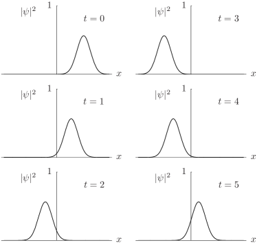
Figure 1: Evolution of the squared modulus of the wave function of a coherent state for the harmonic oscillator.

These coherent states of the harmonic oscillator (and their free field counterparts) have a number of additional interesting properties including the followinggalindo :

1. They are eigenstates of the annihilation operator –that can be written in terms of the position and momentum operators as $\hat{a}=\frac{1}{\sqrt{2}}(\hat{X}+i\hat{P})$– with complex eigenvalue $z$ whose real and imaginary parts encode the initial position and momenta of the classical motion. In terms of $z$ and its complex conjugate $\bar{z}$ we have $\langle z|\hat{X}|z\rangle=\frac{1}{\sqrt{2}}(\bar{z}+z)$ and $\langle z|\hat{P}|z\rangle=\frac{i}{\sqrt{2}}(\bar{z}-z)$. If we start with the condition that $|z\rangle$ is an eigenstate of $\hat{a}$, it is straightforward to express $|z\rangle$ in terms of the energy eigenstates $|n\rangle$:

   $$|z\rangle=\exp(-|z|^{2}/2)\sum_{n=0}^{\infty}\frac{z^{n}}{\sqrt{n!}}|n\rangle.$$ (17)

2. The dispersion of the position and momentum operators in these states $[\langle z|\hat{X}^{2}|z\rangle-\langle z|\hat{X}|z\rangle^{2}]=[\langle z|\hat{P}^{2}|z\rangle-\langle z|\hat{P}|z\rangle^{2}]=\frac{1}{2}$ are constant and saturate the Heisenberg uncertainty inequalities (coherent states define minimal wave packets). It can be seen that coherent states are also minimal with respect to energy and momentum galindo in the sense that $\Delta_{z}H_{0}=|z|$, the characteristic time of the system in the state $|z\rangle$ is $\tau_{z}=1/(2\Delta_{z}H_{0})$, and then $\tau_{z}\Delta_{z}H_{0}=1/2$.

3. The time evolution of the state $|z_{0}\rangle$ is given by

   $$e^{-iT\hat{H}_{0}}|z_{0}\rangle=e^{-iT/2}|e^{-iT}z_{0}\rangle.$$ (18)

   This equation means that as time evolves, the unitary ray defined by a coherent state $|z_{0}\rangle$ at $T=0$ (i.e. the set of vectors of the form $e^{i\theta}|z_{0}\rangle$ with $\theta\in\mathbb{R}$) remains coherent at any time $T$ and is labeled by

   $$z(T)=e^{-iT}z_{0}=x_{0}(T)+ip_{0}(T),$$ (19)

   where the functions $x_{0}(T)$ and $p_{0}(T)$, given by Eq. (5), are the position and momentum of the classical harmonic oscillator as a function of time.

4. The set of coherent states defines a linear, non-orthonormal, overcomplete basis of the Hilbert space for a harmonic oscillator. In particular, we can find a relation of the type

   $$\frac{1}{\pi}\int_{\mathbb{C}}\mathrm{d}^{2}z|z\rangle\langle z|=\mathbb{I}.$$ (20)

   As we can see, the coherent states for the harmonic oscillator satisfy a set of properties that allow us to consider them as semiclassical in the sense that their time evolution closely follows the classical one. They also satisfy interesting properties that render them an important tool in the study of oscillator systems or free field theories.

V Example

As an illustration of these methods, we will answer the question: Can we build appropriate coherent states for a one-particle system with a Hamiltonian of the form $f(H_{0})$ with $H_{0}=\frac{1}{2}(p^{2}+x^{2})$? This case is interesting because if the answer were affirmative, it could be possible to extend the result for interesting field theories such as general relativity reductions of the Einstein-Rosen type. As we will see the answer to this question is in the negative.

We show that it is not possible to build proper coherent states for $f(H_{0})$ by proving that under time evolution the label $z$, which encodes the initial data, cannot evolve according to the classical dynamics dictated by $f(H_{0})$. In terms of the initial data $z_{0}=x_{0}+ip_{0}$ (combined in the complex number $z_{0}$), the classical evolution of the system is obtained from Eq. (13)

$$z(t)=z_{0}\exp\big{(}-itf^{\prime}(|z_{0}|^{2}/2)\big{)}.$$ (21)

So we will require that the state, which we will also label $|z\rangle$ in analogy with the usual coherent states, evolve as

$$\exp(-itf(\hat{H_{0}}))|z\rangle=\exp(i\varphi(t,z))\left|z\exp(-itf^{\prime}(|z|^{2}/2))\right\rangle.$$ (22)

Equation (22) is similar to Eq. (18). Note that we must work with unitary rays so we include an arbitrary phase $\exp(i\varphi(t,z))$. We now expand $|z\rangle$ in the orthonormal basis provided by the energy eigenfunctions $|n\rangle$ of the harmonic oscillator Hamiltonian

$$|z\rangle=\sum_{n=0}^{\infty}\psi_{n}(z)|n\rangle,$$ (23)

where the coefficients $\psi_{n}(z)=\psi_{n}(x+ip)=\psi_{n}(x,p)$ are taken as differentiable functions. Equation (22) becomes

$$\psi_{n}(z)=\exp[i(\varphi(t,z)+tf(E_{n}))]\psi_{n}(z\exp(-itf^{\prime}(|z|^{2}/2))).$$ (24)

If we use the notation $\psi_{n}(x,p)$ for $\psi_{n}(z)$ we can rewrite Eq. (24) as

$$\psi_{n}(x,p) = \exp[i(\varphi(t,z)+tf(E_{n}))]$$

$$\times\psi_{n}\Big{(}x\cos(tf^{\prime}(|z|^{2}/2))+p\sin(tf^{\prime}(|z|^{2}/2)),p\cos(tf^{\prime}(|z|^{2}/2))-x\sin(tf^{\prime}(|z|^{2}/2))\Big{)}.$$

The left-hand side of Eq. (V) does not depend on time, so the time derivative of the right-hand side must be zero. We evaluate this derivative at $t=0$ and obtain the consistency condition

$$f^{\prime}(|z|^{2}/2)\left[p\frac{\partial\psi_{n}}{\partial x}(x,p)-x\frac{\partial\psi_{n}}{\partial p}(x,p)\right]=-i\left[\dot{\varphi}_{0}(z)+f(E_{n})\right]\psi_{n}(x,p),$$ (26)

with $\dot{\varphi}_{0}(z)=\frac{\partial\varphi(0,z)}{\partial t}$. By introducing polar coordinates $x=r\cos\theta$ and $p=r\sin\theta$ we can rewrite Eq. (26) as

$$\frac{\partial\psi_{n}(r,\theta)}{\partial\theta}=i\frac{\dot{\varphi}_{0}(r,\theta)+f(E_{n})}{f^{\prime}(r^{2}/2)}\,\psi_{n}(r,\theta).$$ (27)

Equation (27) can be solved to give

$$\psi_{n}(r,\theta)=c_{n}(r^{2})\exp\left[i\frac{f(E_{n})\theta+X(\theta,r)}{f^{\prime}(r^{2}/2)}\right],$$ (28)

where

$$X(\theta,r)=\!\int\dot{\varphi}_{0}(\theta,r)\,\mathrm{d}\theta,$$ (29)

and $c_{n}(r^{2})$ are arbitrary functions of $r^{2}$. It can be easily checked that for the usual harmonic oscillator, $f(x)=x$ and $E_{n}=n+\frac{1}{2}$, the choice $\varphi(t,z)=-t/2$ gives $\psi_{n}=c_{n}(r^{2})\exp(in\theta)$. The latter can be written as $\psi_{n}(z)=c_{n}(|z|^{2})\exp(in\mathrm{Arg}_{n}(z))$, where $\mathrm{Arg}_{n}$ is a branch of the argument of $z$. With this choice $\exp(in\mathrm{Arg}_{n}(z))$ is independent of the branch chosen for the argument, and we can write $\psi_{n}(z)=c_{n}(|z|^{2})\exp(in\mathrm{Arg}(z))=\tilde{c}_{n}(|z|^{2})z^{n}$ with $\mathrm{Arg}(z)=\{\arctan(p/q)+2k\pi,k\in\mathbb{Z}\}$. This result should be compared with the result $\psi_{n}(z)=e^{-|z|^{2}/2}z^{n}/n!$ corresponding to the harmonic oscillator coherent states. As we can see only part of the dependence on $z$ is fixed by Eq. (22), but the result is compatible with $\psi_{n}(z)=e^{-|z|^{2}/2}z^{n}/n!$. By using the other conditions the full dependence on $z$ can be obtained.

From Eq. (28) we observe that, in general, the result will depend on the branch chosen. This ambiguity is unacceptable so we conclude that it is usually impossible to have a family of coherent states satisfying a condition equivalent to Eq. (22) for the evolution given by $f(H_{0})$. We consider an explicit example using the functional form given by the Hamiltonian of the Einstein-Rosen waves $f(x)=2(1-e^{-x/2})$. The solution (28) for this choice is

$$\psi_{n}(r,\theta)=c_{n}(r^{2})\exp\left(ie^{r^{2}/4}[2(1-e^{-\frac{1}{2}(n+\frac{1}{2})})\theta+X(\theta,r)]\right).$$ (30)

We need to require that

$$\exp\left(ie^{r^{2}/4}[2(1-e^{-\frac{1}{2}(n+\frac{1}{2})})\theta+X(\theta,r)]\right)$$ (31)

be independent of the branch chosen for the argument $\theta$ –otherwise it is not single-valued. However, this requirement is impossible to satisfy because $X(\theta,r)$ is independent of $n$. If we write $\theta=\tilde{\theta}+2k\pi$, we obtain the condition

$$4k\pi e^{r^{2}/4}(1-e^{-\frac{1}{2}(n+\frac{1}{2})})+e^{r^{2}/4}X(\tilde{\theta}+2k\pi,r)\equiv e^{r^{2}/4}X(\tilde{\theta},r)\quad(\mathrm{mod}\,2\pi).$$ (32)

If we consider Eq. (32) for two different numbers $n$ and $m$, the difference between them gives

$$4\pi k\,e^{r^{2}/4}\left(e^{-\frac{1}{2}(n+\frac{1}{2})}-e^{-\frac{1}{2}(m+\frac{1}{2})}\right)\equiv 0\quad(\mathrm{mod}\,2\pi)$$ (33)

for all $m$ and $n$ which is impossible.

VI Conclusions

We have described the classical and quantum dynamics of systems with Hamiltonians that are functions of other solvable Hamiltonians and compared the cases $H_{0}$ and $f(H_{0})$. Classically the states evolve in very similar ways and follow the same phase space orbits although with different time parametrizations. In contrast, their quantum evolution is qualitatively different due to the appearance of non-trivial relative phases. We discussed this issue by analyzing the existence of coherent states and their properties for functionally related Hamiltonians. In particular, we gave a proof of the impossibility of constructing coherent states that satisfy the four conditions in Sec. IV for general Hamiltonians of the form $H=f(H_{0})$, with $H_{0}$ corresponding to the harmonic oscillator. This case is especially significant because of the role played by harmonic oscillators in the description of free quantum field theories.

By relaxing some of the conditions defining coherent states for the harmonic oscillator, we can conceivably find a set of suitable semiclassical states for the more complicated dynamics given by $f(H_{0})$. Our analysis does not exclude this possibility, but suggests that the definition that we must adopt will require major changes in the conditions that are satisfied by the familiar coherent states.

- (1) J. Banerji, “Nonlinear wave packet dynamics of coherent states,” Pramana J. Phys. 56, 267–280 (2001).
- (2) W. Leoński, “Periodic behaviour of displaced Kerr states,” Acta Phys. Slovaca 48, 371–378 (1998).
- (3) A. Einstein and N. Rosen, “On gravitational waves,” J. Franklin Inst. 223, 43–54 (1937).
- (4) A. Ashtekar and M. Varadarajan, “Striking property of the gravitational Hamiltonian,” Phys. Rev. D 50, 4944–4956 (1994).
- (5) J. F. Barbero G., I. Garay, and E. J. S. Villaseñor, “Probing quantized Einstein-Rosen waves with massless scalar matter,” Phys. Rev. D 74, 044004-1–22 (2006).
- (6) M. Reed and B. Simon, Methods of Modern Mathematical Physics: Functional Analysis (Academic Press, London 1980), Vol. 1.
- (7) A. Galindo and P. Pascual, Quantum Mechanics (Springer-Verlag, Berlin 1991), Vols. I and II.
- (8) A. Messiah, Quantum Mechanics (Dover, N.Y. 1999).