Drift of slow variables in slow-fast Hamiltonian systems

Abstract

We study the drift of slow variables in a slow-fast Hamiltonian system with several fast and slow degrees of freedom. For any periodic trajectory of the fast subsystem with the frozen slow variables we define an action. For a family of periodic orbits, the action is a scalar function of the slow variables and can be considered as a Hamiltonian function which generates some slow dynamics. These dynamics depend on the family of periodic orbits.

Assuming the fast system with the frozen slow variables has a pair of hyperbolic periodic orbits connected by two transversal heteroclinic trajectories, we prove that for any path composed of a finite sequence of slow trajectories generated by action Hamiltonians, there is a trajectory of the full system whose slow component shadows the path.

1 Introduction

We consider a slow-fast Hamiltonian system described by a smooth Hamiltonian function $H(p,q,v,u;\varepsilon)\,.$ This system is slow-fast due to a small parameter in the symplectic form

$$\Omega=dp\wedge dq+\frac{1}{\varepsilon}dv\wedge du\,.$$

Therefore the equations of motion take the form

$$\begin{array}[]{ll}\displaystyle\dot{q}=\frac{\partial H}{\partial p}\,,&\displaystyle\dot{p}=-\frac{\partial H}{\partial q}\,,\\[10.0pt] \displaystyle\dot{u}=\varepsilon\frac{\partial H}{\partial v}\,,&\displaystyle\dot{v}=-\varepsilon\frac{\partial H}{\partial u}\,.\end{array}$$ (1)

Equations of this form often arise after rescaling a part of the variables in a Hamiltonian system with the standard symplectic form.

The variable $(p,q)$ are called fast and $(v,u)$ are slow. We assume that the system has $m+d$ degrees of freedom, where $m$ is the number of fast degrees of freedom and $d$ is the number of slow ones.

After substituting $\varepsilon=0$ into equation (1) we see that the values of $(v,u)$ remain constant in time and the system can be interpreted as a family of Hamiltonian systems with $m$ degrees of freedom which depends on $2d$ parameters. We call it a frozen system:

$$\begin{array}[]{ll}\displaystyle\dot{q}=\frac{\partial H}{\partial p}\,,&\displaystyle\dot{p}=-\frac{\partial H}{\partial q}\,,\\[10.0pt] \displaystyle\dot{u}=0\,,&\displaystyle\dot{v}=0\,.\end{array}$$ (2)

The case when the fast system has one degree of freedom is relatively well understood. Indeed, in this case the frozen system typically represents a fast oscillator. The averaging method can be used to eliminate the dependence on the fast oscillations from the slow system. Therefore trajectories of the slow system are close to trajectories of an autonomous system with $2d$ degrees of freedom over very long time intervals (see e.g. [1, 2]).

Points of equilibria of the frozen system form surfaces called slow manifolds. Normally hyperbolic slow manifolds persists and normally elliptic slow manifolds do not in general. In both cases the dynamics in a neighbourhood of a slow manifold can be described using normal forms (for a discussion see e.g. [5]).

The case when the fast system has more than one degree of freedom is notably more difficult. The effect of the fast system on the slow variables strongly depends on the dynamics of the fast system. If the frozen fast system oscillates with a constant vector of frequencies, generalisations of the averaging method can be used [8, 9]. The averaging method can be also used if the frozen system is uniformly hyperbolic [4] or, more generally, if the frozen system is ergodic and time averages converge sufficiently fast to space averages [7]. In all these cases the dynamics of the slow variables is described, in the leading order, by the vector field obtained by taking an average of the slow component of (1) over the space of fast variables

$$\dot{u}=\varepsilon\left<\frac{\partial H}{\partial v}\right>\,,\qquad\dot{v}=-\varepsilon\left<\frac{\partial H}{\partial u}\right>\,.$$ (3)

This approximation strongly relies on the fact that in an ergodic system the time average over a trajectory equals the space average for almost all trajectories. The approximation error strongly depends on the rate of convergence for time averages. If the number of fast degrees of freedom is larger than one, there is no reason to expect that the time average over a periodic orbit converges to the average over the space. Therefore we should expect that the slow component of a trajectory whose fast component stays near a periodic orbit of the frozen system may strongly deviate from the averaged dynamics described by (3). Moreover, we note that periodic orbits are dense in the case of an Anosov system.

In this paper we assume that the frozen system has a compact invariant set bearing chaotic dynamics of horseshoe type created by transversal heteroclinics between two saddle periodic orbits. This situation typically arises when a periodic orbit has a transversal homoclinic.

In this invariant set hyperbolic periodic orbits are dense and every two periodic orbits are connected by a heteroclinic orbit. We select a finite subset of periodic orbits with relatively short periods. We construct trajectories of the full system which switch between neighbourhoods of the periodic orbits in a prescribed way. We show that the slow component of such trajectories drifts in a way quite similar to trajectories of a random Hamiltonian dynamical system with $2d$ degrees of freedom.

The trajectories constructed in this paper strongly deviate from the averaged dynamics. We think this mechanism is responsible for the largest possible rates of deviation.

A similar construction is used in [6] for studying drift of the enrgy in a Hamiltonian system which depends on time explicitly and slowly. In particular, it was shown in [6] that switching between fast periodic orbits indeed provides the fastest rate of energy growth in several situations.

The rest of the paper has the following structure. In Section 2 we state our main theorem and discuss its application to systems with one slow degree of freedom. In Section 3 we describe slow dynamics of the full system (1) near a family of periodic orbits of the frozen system. The description is based on an action associated with the frozen periodic orbits and can be of independent interest. The central ingredient of the proof of the main theorem is preservation of normally hyperbolic manifolds formed by families of uniformly hyperbolic orbits of the frozen system which is explained in Section 4. In this section we explain how symbolic dynamics can be used to describe the dynamics of the full system restricted to an invariant subset close to the hyperbolic invariant set of the frozen system. The discussion is based on ideas of [6]. Section 5 analyses the long time behaviour of the slow component of the full dynamics. The last section of the paper finishes the proof of the main theorem.

2 Accessibility and drift of slow variables

The total energy is preserved, so we study the dynamics on a single energy level. Without any loss in generality we may consider the dynamics in the zero energy level

$${\cal M}_{\varepsilon}=\{\,H(p,q,v,u;\varepsilon)=0\,\}\,.$$

First we state our assumptions on the dynamics of the frozen system. Let $D\subset{\mathbb{R}}^{2d}$ be in a bounded domain. We assume

• the frozen system has two smooth families of hyperbolic periodic orbits $L_{c}(v,u)\subset{\cal M}_{0}$ defined for all $(v,u)\in D$, $c\in\{\,a,b\,\}$.

• the frozen system has two smooth families of transversal heteroclinic orbits:

  $$\Gamma_{ab}(v,u) \subset W^{u}(L_{a}(v,u))\cap W^{s}(L_{b}(v,u))\,,$$

  $$\Gamma_{ba}(v,u) \subset W^{u}(L_{b}(v,u))\cap W^{s}(L_{a}(v,u))\,,\qquad\forall(v,u)\in D\,.$$

We note that under these assumptions the frozen system has a family of uniformly hyperbolic invariant transitive sets $\Lambda_{(v,u)}$, also known as Smale horseshoes. For every $(v,u)\in D$, this set contains a countable number of saddle periodic orbits, which are dense in $\Lambda_{(v,u)}$. Moreover, every two periodic orbits in $\Lambda_{(v,u)}$ are connected by a transversal heteroclinic orbit, which also belongs to $\Lambda_{(v,u)}$. It is well known that the dynamics on the Smale horseshoe can be described using the language of Symbolic Dynamics. We define

$$\Lambda:=\bigcup_{(v,u)\in D}\Lambda_{(v,u)}\,.$$

Before stating our main theorem we give a couple of definitions.

Definition 1

The action of a periodic orbit $L_{c}$ is defined by the integral

$$J_{c}(v,u):=\oint_{L_{c}(v,u)}p\,dq\,.$$

The function $J_{c}$ is independent of the fast variables and can be considered itself as a Hamiltonian function which generates some slow dynamics of $(v,u)$ variables:

$$v^{\prime}=-\frac{1}{T_{c}}\frac{\partial J_{c}}{\partial u}\,,\qquad u^{\prime}=\frac{1}{T_{c}}\frac{\partial J_{c}}{\partial v}\,,$$ (4)

where ^′ stands for the derivative with respect to the slow time $\tau=\varepsilon t$, and $T_{c}$ is the period of $L_{c}$. System (4) is Hamiltonian with the symplectic form $\omega_{c}=T_{c}(v,u)dv\wedge du$. Alternatively the equations can be interpreted as a result of a time scaling in a standard Hamiltonian system.

In the next sections we will show that for properly chosen initial conditions the slow component of the corresponding trajectory of (1) oscillates near a trajectory of this slow Hamiltonian system.

Inside the Smale horseshoe there are infinitely many periodic orbits connected by transversal heteroclinics. Each periodic orbit has an action associated with it. We select a finite subset of periodic orbits and consider the collection of their actions. In general we should expect all those actions to be different.

In this paper we prove that there are trajectories of the full system such that their slow components follow any finite path composed of segments of slow trajectories generated by actions. Those trajectories of the full system shadow a chain composed of the periodic orbits and heteroclinic trajectories and spend most of the time near periodic orbits of the frozen system.

Let us give a definition of an accessible path and then state the theorem. Consider a finite family of functions $J_{k}:D\to{\mathbb{R}}$, $k=1,\ldots,n$. Let $\Phi^{\tau}_{k}$ be the Hamiltonian flow with Hamiltonian function $J_{k}$ and the symplectic form $\omega_{k}=T_{k}(v,u)dv\wedge du$ where $T_{k}>0$ is the period of the corresponding orbit. For every point $z=(v,u)\in D$ we define

$$\sigma_{k}(z)=\sup\{\,\tau:\Phi_{k}^{\tau^{\prime}}(z)\in D\quad\mbox{for all $\tau^{\prime}\in(0,\tau)$}\,\}\,,$$

which is the time required to leave the domain $D$. If the trajectory is defined for all $\tau>0$ we set $\sigma_{k}(z)=+\infty$. Obviously, $\sigma_{k}(z)>0$ for any $z$ and $k$ due to openness of $D$.

Definition 2

We say that $\Gamma:[0,T]\to D$ is an accessible path if $\Gamma$ is a piecewise smooth curve composed from a finite number of forward trajectories of the Hamiltonian systems generated by $J_{k}$.

More formally, $\Gamma$ is an accessible path if there are $0=\tau_{0}<\tau_{1}<\dots<\tau_{N}=T$ such that the sequence of points $z_{i}:=\Gamma(\tau_{i})$ breaks the curve $\Gamma$ into trajectories, i.e., for every $i<N$, there is $k_{i}$, $1\leq k_{i}\leq n$, such that for $\tau\in[\tau_{i},\tau_{i+1}]$

$$\Gamma(\tau)=\Phi_{k_{i}}^{\tau-\tau_{i}}(z_{i})\,.$$

Of course, the curve $\Gamma$ is well defined only if

$$0<\tau_{i+1}-\tau_{i}<\sigma_{k_{i}}(z_{i})$$

which ensures that the trajectories do not leave the domain $D$.

Theorem 1

If $D$ is a bounded domain in ${\mathbb{R}}^{2d}$, the frozen fast system satisfies assumptions [A1] and [A2], $\{J_{k}\}_{k=1}^{n}$ is a set of actions corresponding to a finite set of frozen periodic orbits in $\Lambda$, and $\Gamma$ is an accessible path, then there is a constant $C_{0}>0$ and $\varepsilon_{0}>0$ such that for every $\varepsilon<\varepsilon_{0}$ there is a trajectory of the full system (1) such that its slow component $z(t)$ satisfies

$$\|z(t)-\Gamma(\varepsilon t)\|<C_{0}\varepsilon$$

provided $0\leq t\leq\varepsilon^{-1}T$.

Definition 3

For any $z_{0},z_{1}\in D$, we say that $z_{1}$ is accessible from $z_{0}$ via the system $\{J_{k}\}$ if there is an accessible path such that $\Gamma(0)=z_{0}$ and $\Gamma(T)=z_{1}$.

In the case $d=1$ the accessibility property has a simple geometrical meaning since trajectories of the Hamiltonian systems generated by $J_{k}$ are level lines of the functions $J_{k}$. In this case the theorem provides trajectories which follow segments of the level lines. The main obstacle for the drift in the slow space is provided by level lines common for all $J_{k}$.

Corollary 1

Consider actions generated by two periodic orbits, $a$ and $b$. Those level lines of $J_{a,b}$, which are inside $D$, are closed curves. The non-singular level lines form rings (or disks), $D_{a}$ and $D_{b}$. Let $V=D_{a}\cap D_{b}\subset D$. If $J_{a}$ and $J_{b}$ do not have common level lines, then any point $z_{1}\in V$ is accessible from any point $z_{0}\in V$.

Corollary 2

Under the same assumptions. Let us take any finite family of open sets $V_{i}\subset V$, which do not depend on $\varepsilon$. Then for all sufficiently small $\varepsilon$, there is a trajectory which visits all the sets $V_{i}$.

If the energy set ${\cal M}_{\varepsilon}$ is compact the slow dynamics never leaves a bounded set. If at the same time $D$ is a connected set, natural questions arise: Is there a point in $D$ which is not accessible from every other point in $D$? Is there a trajectory such that its slow component is dense in $D$?

3 Actions and first return maps near periodic orbits of the frozen system

Now consider the cylinder formed by periodic orbits of the frozen system:

$$S_{c,0}=\bigcup_{(v,u)\in D}L_{c}(v,u)\subset{\cal M}_{0}\,.$$ (5)

Let $\gamma_{\varepsilon}$ denote a trajectory of the full system (1) and $\pi_{s}:{\mathbb{R}}^{2m+2d}\to{\mathbb{R}}^{2d}$ the projection on the slow variables.

In the next section we will prove that some trajectories stay in a neighbourhood of $S_{c,0}$ for a very long time and provide a detailed description for them. In this section we show that in this case the evolution of the slow component $\pi_{s}\gamma_{\varepsilon}$ approximately follows a trajectory of the slow Hamiltonian flow $\Phi_{c}^{\varepsilon t}$ generated by the action $J_{c}$.

Lemma 1

Let $L_{c}$ be a family of periodic orbits of the frozen system. If $\gamma_{\varepsilon}$ is a family of solutions of the full system (1) such that

• there are $z_{0}\in D$ and $C_{0}>0$ such that

  $$\|\pi_{s}\gamma_{\varepsilon}(0)-z_{0}\|<C_{0}\varepsilon,$$ (6)

• there are constants $C_{1}>0$ and $\tau_{0}<\sigma_{c}(z_{0})$ such that

  $$\mathrm{dist}(\gamma_{\varepsilon}(t),S_{c,0})\leq C_{1}\varepsilon\qquad\forall t\in[0,\varepsilon^{-1}\tau_{0}],$$ (7)

then there is $C_{2}>0$ such that

$$\|\pi_{s}\gamma_{\varepsilon}(t)-\Phi_{c}^{\varepsilon t}(z_{0})\|\leq C_{2}\varepsilon$$ (8)

for all $t\in[0,\varepsilon^{-1}\tau_{0}]$.

Proof. We write $(p_{c}(t,v,u),q_{c}(t,v,u))$ to denote a periodic solution of the frozen system and use $T_{c}(v,u)$ for the corresponding period:

$$\begin{array}[]{rcl}p_{c}(t+T_{c}(v,u),v,u)&\equiv&p_{c}(t,v,u)\,,\\ q_{c}(t+T_{c}(v,u),v,u)&\equiv&q_{c}(t,v,u)\,.\end{array}$$ (9)

Then the action of the periodic orbit $L_{c}$ is given by the following integral

$$J_{c}(v,u)=\int_{0}^{T_{c}}p_{c}\frac{\partial q_{c}}{\partial t}\,dt\,.$$ (10)

Since $L_{c}$ belongs to the zero energy level we have a useful identity:

$$H(p_{c}(t,v,u),q_{c}(t,v,u),v,u;0)=0$$ (11)

for all $(v,u)\in D$ and all $t\in{\mathbb{R}}$.

Let $\Sigma$ denote a smooth hypersurface in ${\mathbb{R}}^{2m+2d}$ transversal to the flow of the frozen system such that every periodic orbit of the family $L_{c}$ has exactly one intersection with $\Sigma$. Let $M_{i}=\gamma_{\varepsilon}(t_{i})$ be a sequence of consecutive intersections of $\gamma_{\varepsilon}$ with $\Sigma$ and consider the slow components of those points: $\hat{z}_{i}:=\pi_{s}M_{i}$.

We note that inequality (7) and the smooth dependence of $p_{c}(s,z),q_{c}(s,z)$ on $z$ imply that there is $C_{3}>0$ such that for every $i$ there is $s_{i}$ such that

$$\|M_{i}-(p_{c}(s_{i},\hat{z}_{i}),q_{c}(s_{i},\hat{z}_{i}),\hat{z}_{i})\|\leq C_{1}\varepsilon\,.$$

Since solutions of differential equations depend smoothly on the initial conditions and vector field, the segment of $\gamma_{\varepsilon}(t)$, $t_{i}\leq t\leq t_{i+1}$ is close to $L_{c}(\hat{z}_{i})$:

$$\gamma_{\varepsilon}(t)=(p_{c}(s_{i}+t-t_{i},\hat{z}_{i}),q_{c}(s_{i}+t-t_{i},\hat{z}_{i}),\hat{z}_{i})+O(\varepsilon)$$ (12)

and the time of the first return to the section $\Sigma$ is close to the period of the frozen trajectory:

$$t_{i+1}-t_{i}=T_{c}(\hat{z}_{i})+O(\varepsilon).$$ (13)

Now we estimate the displacement $\hat{z}_{i+1}-\hat{z}_{i}$. We write $\hat{z}_{i}=(v,u)$ and $\hat{z}_{i+1}=(\bar{v},\bar{u})$ to shorten the notation. Integrating the slow component of the vector field along the exact trajectory and using (1) we conclude

$$\begin{array}[]{rclcl}\bar{u}-u&=&\displaystyle\int_{t_{i}}^{t_{i+1}}\dot{u}dt&=&\displaystyle\varepsilon\int_{0}^{T_{c}(v,u)}\left.\frac{\partial H}{\partial v}\right|_{p_{c}(t,v,u),q_{c}(t,v,u),v,u}dt+O(\varepsilon^{2})\,,\\ \bar{v}-v&=&\displaystyle\int_{t_{i}}^{t_{i+1}}\dot{v}dt&=&\displaystyle-\varepsilon\int_{0}^{T_{c}(v,u)}\left.\frac{\partial H}{\partial u}\right|_{p_{c}(t,v,u),q_{c}(t,v,u),v,u}dt+O(\varepsilon^{2})\,,\end{array}$$ (14)

where the error terms come from replacing the exact trajectory by the frozen one and from the difference in the return time, see (12) and (13). The integrals in the right hand side can be expressed in terms of derivatives of the action defined by integral (10). Indeed, differentiating (10) with respect to $u$, integrating by parts and taking into account (9), we get

$$\frac{\partial J_{c}}{\partial u} = \int_{0}^{T_{c}}\left(\frac{\partial p_{c}}{\partial u}\frac{\partial q_{c}}{\partial t}-\frac{\partial q_{c}}{\partial u}\frac{\partial p_{c}}{\partial t}\right)dt$$

$$= \int_{0}^{T_{c}}\left(\frac{\partial p_{c}}{\partial u}\frac{\partial H}{\partial p}+\frac{\partial q_{c}}{\partial u}\frac{\partial H}{\partial q}\right)dt\,.$$

Then differentiating identity (11) we get

$$\frac{\partial p_{c}}{\partial u}\frac{\partial H}{\partial p}+\frac{\partial q_{c}}{\partial u}\frac{\partial H}{\partial q}=-\frac{\partial H}{\partial u}\,,$$

where the derivatives are evaluated at $(p_{c}(t,v,u),q_{c}(t,v,u),v,u)$. Consequently

$$\frac{\partial J_{c}}{\partial u}=-\int_{0}^{T_{c}(v,u)}\left.\frac{\partial H}{\partial u}\right|_{p_{c}(t,v,u),q_{c}(t,v,u),v,u}dt\,.$$

Repeating these arguments with $u$ replaced by $v$ we also get

$$\frac{\partial J_{c}}{\partial v}=-\int_{0}^{T_{c}(v,u)}\left.\frac{\partial H}{\partial v}\right|_{p_{c}(t,v,u),q_{c}(t,v,u),v,u}dt\,.$$

Substituting the last two equalities into (14) we arrive to

$$\bar{u}=u-\varepsilon\frac{\partial J_{c}}{\partial v}+O(\varepsilon^{2})\,,\qquad\bar{v}=v+\varepsilon\frac{\partial J_{c}}{\partial u}+O(\varepsilon^{2})\,.$$ (15)

We see that the displacement between two consecutive intersections of $\gamma_{\varepsilon}$ with section $\Sigma$ is approximated by the time-$\varepsilon T_{c}$ shift along a trajectory of the Hamiltonian vector field (4) generated by the Hamiltonian function $J_{c}$:

$$\hat{z}_{i+1}=\hat{z}_{i}+\Phi_{c}^{\varepsilon T_{c}}(\hat{z}_{i})+O(\varepsilon^{2})\,.$$

Inequality (6) implies that $\hat{z}_{0}=z_{0}+O(\varepsilon)$. Then a rather standard stability estimate can be used to show

$$\hat{z}_{i}=\Phi_{c}^{i\varepsilon T_{c}}(z_{0})+O(\varepsilon)\qquad\mbox{for $0\leq i\leq\varepsilon^{-1}\tau_{0}$.}$$ (16)

Finally, we note that $\hat{z}_{i}=\pi_{s}\gamma_{\varepsilon}(t_{i})$ where $t_{i}=iT_{c}+O(\varepsilon i)$ due to (13). Between intersections with $\Sigma$ the slow component $\pi_{s}\gamma_{\varepsilon}$ changes by a value of the order of $O(\varepsilon)$. Therefore the estimate is extendable to values of $t$ between the intersections and (8) follows immediately. $\Box$

We note that $J_{c}$ is preserved by $\Phi_{c}^{\tau}$ and therefore $J_{c}\circ\pi_{s}$ is an adiabatic invariant for the restriction of the full dynamics on a neighbourhood of $S_{c,0}$.

In general, we do not expect the estimates to be valid on time intervals longer than stated by Lemma 1. For example, note that a trajectory of $J_{c}$ may leave the domain $D$ in finite time.

It is interesting that under additional assumptions $\hat{J}_{c}(t):=J_{c}(\pi_{s}\gamma_{\varepsilon}(t))$ may stay near its initial value, $\hat{J}_{c}(0)$, for much longer time.

Indeed, consider the case of one slow degree of freedom, $d=1$, and suppose that level lines of $J_{c}$ are closed curves on the plane of $(v,u)$ variables. Then $\sigma_{c}(z)=+\infty$ for all $z\in D$. In the next section we will show that the full system has a locally invariant cylinder $S_{c,\varepsilon}$ close to $S_{c,0}$. Then equations (14) describe a Poincaré map on the section defined by intersection of $S_{c,\varepsilon}$ and $\Sigma$. In the case of one slow degree of freedom we may suppose that the map (14) satisfies assumptions of the KAM theorem, then $\hat{J}_{c}(t)$ will stay close to its initial value forever. Indeed, under these assumptions the trajectories on $S_{c,\varepsilon}$ are trapped between two KAM tori.

We also note that averaging theory can be used to study the dynamics on $S_{c,\varepsilon}$ for $d\geq 1$.

4 Dynamics of the frozen system and normal hyperbolicity

The following arguments are based on [6]. Let $w=(p,q)$ and $z=(v,u)$ to shorten notation. Then the frozen system (2) has the form

$$\dot{w}=G(w,z)\,,$$ (17)

where $G$ is expressed in terms of partial derivatives of $H$ for $\varepsilon=0$. The Hamiltonian function $H(w,z)$ is an integral of system (17).

Let system (17) have two smooth families of saddle periodic orbits $L_{a}:w=w_{a}(t,z)$ and $L_{b}:w=w_{b}(t,z)$ for all $z\in D$. Assume that both families belong to the zero energy level ${\cal M}_{0}$. Take a pair of smooth cross-sections, $\Sigma_{a}$ and $\Sigma_{b}$, which are transverse to the vector field and such that each periodic trajectory $L_{a}(z)$ and $L_{b}(z)$ has exactly one point of intersection with the corresponding section. Denote the Poincaré map on $\Sigma_{c}$ near $L_{c}$ as $\Pi_{cc}$ ($c=a,b$). The Poincaré map is smooth and depends smoothly on $z$.

We assume that for all $z\in D$ the frozen system has a pair of transversal heteroclinic orbits: $\Gamma_{ab}\subseteq W^{u}(L_{a})\cap W^{s}(L_{b})$ and $\Gamma_{ba}\subseteq W^{u}(L_{b})\cap W^{s}(L_{a})$.

Let $\Pi_{ab}$ and $\Pi_{ba}$ be maps defined on subsets of $\Sigma_{a}$ and $\Sigma_{b}$ by following orbits close to $\Gamma_{ab}$ and $\Gamma_{ba}$, respectively. Therefore $\Pi_{ab}$ acts from some open set in $\Sigma_{a}$ into an open set in $\Sigma_{b}$, while $\Pi_{ba}$ acts from an open set in $\Sigma_{b}$ into an open set in $\Sigma_{a}$. There is a certain freedom in the definition of the maps $\Pi_{ab}$ and $\Pi_{ba}$. Indeed, each of these maps acts from a neighbourhood of one point of a heteroclinic orbit to a neighbourhood of another point of the same orbit, therefore different choices of the points lead to different maps.

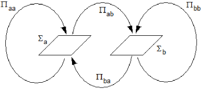
Figure 1: Poincaré maps near two periodic orbits

When the maps are fixed, every orbit that lies entirely in a sufficiently small neighbourhood of the heteroclinic cycle $L_{a}\cup L_{b}\cup\Gamma_{ab}\cup\Gamma_{ba}$ corresponds to a uniquely defined sequence of points $M_{i}\in\Sigma_{a}\cup\Sigma_{b}$ such that

$$M_{i+1}=\Pi_{\xi_{i}\xi_{i+1}}M_{i}$$

where

$$\xi_{i}=c\;\mbox{ if }\;M_{i}\in\Sigma_{c}\;\;(c\in\{\,a,b\,\}).$$

In this way the trajectory of the frozen system defines a sequence $\{\xi_{i}\}_{i=-\infty}^{i=+\infty}$ which is called the code of the orbit.

The periodic orbits $L_{a}$ and $L_{b}$ are saddle and the intersections of the stable and unstable manifolds of $L_{a}$ and $L_{b}$ that create the heteroclinic orbits are transverse due to the assumptions [A1] and [A2]. Consequently (cf. [3]), one can choose the maps $\Pi_{ab}$ and $\Pi_{ba}$ and define coordinates $(x,y,z)$ in $\Sigma_{a}$ and $\Sigma_{b}$ in such a way that the following holds.

• $\Sigma_{c}\cap{\cal M}_{0}$ is diffeomorphic to the product $X_{c}\times Y_{c}\times D$ where $X_{c}$ and $Y_{c}$ are balls in $\mathbb{R}^{m-1}$ of a radius $R>0$ centred around the origin.

• For each pair $c,c^{\prime}\in\{\,a,b\,\}$ the Poincaré map $\Pi_{cc^{\prime}}$ can be written in the following “cross-form” [12]: there exist smooth functions $f_{cc^{\prime}},g_{cc^{\prime}}:X_{c}\times Y_{c^{\prime}}\rightarrow X_{c^{\prime}}\times Y_{c}$ such that a point $M(x,y,z)\in\Sigma_{c}$ is mapped to $\bar{M}(\bar{u},\bar{w},z)\in\Sigma_{c^{\prime}}$ by the map $\Pi_{cc^{\prime}}$ if and only if

  $$\bar{x}=f_{cc^{\prime}}(x,\bar{y},z),\qquad y=g_{cc^{\prime}}(x,\bar{y},z).$$ (18)

• There exists $\lambda<1$ such that

  $$\left\|\frac{\partial(f_{cc^{\prime}},g_{cc^{\prime}})}{\partial(x,\bar{y})}\right\|\leq\lambda<1\,,$$ (19)

  where the norm of the Jacobian matrix corresponds to $\max\{\|x\|,\|y\|\}$.

Inequality (19) implies that for a fixed $z\in D$ the set $\Lambda_{z}$ of all orbits that lie entirely in a sufficiently small neighbourhood of the heteroclinic cycle $L_{a}\cup L_{b}\cup\Gamma_{ab}\cup\Gamma_{ba}$ in the energy level ${\cal M}_{0}$ is hyperbolic, a horseshoe. Moreover, one can show that the orbits in $\Lambda_{z}$ are in one-to-one correspondence with the set of all sequences of $a$’s and $b$’s, i.e. for every sequence $\{\xi_{i}\}_{i=-\infty}^{i=+\infty}$ there exists one and only one orbit in $\Lambda_{z}$ which has this sequence as its code.

Indeed, take any orbit from $\Lambda_{z}$ and denote by $M_{i}(x_{i},y_{i},z)$ the sequence of its intersections with the cross sections. Equation (18), implies that the orbit has a code $\{\xi_{i}\}_{i=-\infty}^{i=+\infty}$ if and only if the coordinates of $M_{i}$ satisfy the equations

$$x_{i+1}=f_{\xi_{i}\xi_{i+1}}(x_{i},y_{i+1},z),\qquad y_{i}=g_{\xi_{i}\xi_{i+1}}(x_{i},y_{i+1},z)\,.$$

Therefore the sequence $\{\,(x_{i},y_{i})\,\}_{i=-\infty}^{+\infty}$ is a fixed point of the operator

$$\{\,(x_{i},y_{i})\,\}_{i=-\infty}^{+\infty}\mapsto\{\,(f_{\xi_{i-1}\xi_{i}}(x_{i-1},y_{i},z),g_{\xi_{i}\xi_{i+1}}(x_{i},y_{i+1},z)\,\}_{i=-\infty}^{+\infty}\,.$$ (20)

Equation (19) implies this operator is a contraction of the space $\prod_{i=-\infty}^{+\infty}X_{\xi_{i}}\times Y_{\xi_{i}}$, hence the existence and uniqueness of the orbit with the code $\{\xi_{i}\}_{i=-\infty}^{i=+\infty}$ follow (see e.g. [11]).

Moreover, the fixed point of a smooth contracting map depends smoothly on parameters. Consequently the orbit depends smoothly on $z$ and the derivatives of $(x_{i}(z,\xi),y_{i}(z,\xi))$ are bounded uniformly for all $i$.

Lemma 2

If the Poincaré maps satisfy assumptions [H1]–[H3], then for any two code sequences $\xi^{(1)}=\{\xi^{(1)}_{i}\}_{i=-\infty}^{+\infty}$ and $\xi^{(2)}=\{\xi^{(2)}_{i}\}_{i=-\infty}^{+\infty}$, which satisfy

$$\xi^{(1)}_{i}=\xi^{(2)}_{i}\qquad\mbox{for $|i|\leq n$}$$

the corresponding intersections with the cross sections are bounded by

$$\max\left\{\,\bigl{\|}x_{i}(z,\xi^{(1)})-x_{i}(z,\xi^{(2)})\bigr{\|},\ \bigl{\|}y_{i}(z,\xi^{(1)})-y_{i}(z,\xi^{(2)})\bigr{\|}\,\right\}\leq 2R\lambda^{n-|i|}\,,$$ (21)

where the constants $R>0$ and $\lambda\in(0,1)$ are defined in [H1] and [H3] respectively and do not depend on the sequences $\xi^{(1,2)}$.

Proof. First we note, that

$$\max\left\{\,\bigl{\|}x_{i}(z,\xi^{(1)})-x_{i}(z,\xi^{(2)})\bigr{\|},\ \bigl{\|}y_{i+1}(z,\xi^{(1)})-y_{i+1}(z,\xi^{(2)})\bigr{\|}\,\right\}$$ (22)

$$\leq \lambda\max\left\{\,\bigl{\|}x_{i+1}(z,\xi^{(1)})-x_{i+1}(z,\xi^{(2)})\bigr{\|},\ \bigl{\|}y_{i}(z,\xi^{(1)})-y_{i}(z,\xi^{(2)})\bigr{\|}\,\right\}$$

for $-n\leq i<n$. Since none of the normes involved exceeds $2R$ we immediately conclude that

$$\max\left\{\,\bigl{\|}x_{i}(z,\xi^{(1)})-x_{i}(z,\xi^{(2)})\bigr{\|},\ \bigl{\|}y_{i+1}(z,\xi^{(1)})-y_{i+1}(z,\xi^{(2)})\bigr{\|}\,\right\}\leq 2R\lambda\,.$$ (23)

Then the following estimate is true for $n^{\prime}=1$

$$\max\bigl{\{}\,\bigl{\|}x_{i}(z,\xi^{(1)})-x_{i}(z,\xi^{(2)})\bigr{\|},\ \bigl{\|}y_{i+1}(z,\xi^{(1)})-y_{i+1}(z,\xi^{(2)})\bigr{\|}\,\bigr{\}}$$

$$\quad\leq 2R\left\{\begin{array}[]{ll}\lambda^{n^{\prime}-i}&\mbox{for $0\leq i<n^{\prime}$}\\ \lambda^{n^{\prime}+1+i}&\mbox{for $-n^{\prime}-1<i<0$}\end{array}\right.\,.$$ (26)

We continue inductively in $n^{\prime}$. Assuming that the estimate (4) holds for $n^{\prime}$ replaced by $n^{\prime}-1$ we check the upper bounds for all $2n^{\prime}+1$ different values of $i$ in the order of decreasing of $|i|$. On each step we use the contraction property (22) and the sharper of upper bounds (4) and (23). In the case $n^{\prime}=n$,

$$\max\bigl{\{}\,\bigl{\|}x_{n}(z,\xi^{(1)})-x_{n}(z,\xi^{(2)})\bigr{\|},\ \bigl{\|}y_{-n}(z,\xi^{(1)})-y_{-n}(z,\xi^{(2)})\bigr{\|}\,\bigr{\}}\leq 2R$$

is used instead of (23). Then (21) follows directly from the last upper bound and (4) taken with $n^{\prime}=n$. $\Box$

Now let us consider the full system (1) for a small $\varepsilon>0$. Since the vector field depends smoothly on $\varepsilon$, the Poincaré maps $\Pi_{cc^{\prime}}:\Sigma_{c}\rightarrow\Sigma_{c^{\prime}}$ are still defined and can be written in the following form:

$$\left\{\begin{array}[]{ll}\displaystyle\bar{x}=f_{cc^{\prime}}(x,\bar{y},z,\varepsilon),\qquad y=g_{cc^{\prime}}(x,\bar{y},z,\varepsilon)\\[6.0pt] \displaystyle\bar{z}=z+\varepsilon\phi_{cc^{\prime}}(x,\bar{y},z,\varepsilon),\end{array}\right.$$ (27)

where $f,g,\phi$ are bounded along with the first derivatives and $f,g$ satisfy (19).

For technical reasons we need to assume that the domain $D$ is invariant under the Poincaré map, i.e., $\phi_{cc^{\prime}}(x,\bar{y},z,\varepsilon)\equiv 0$ if $z\in\partial D$. If this is not the case, then we modify $\phi_{cc^{\prime}}$ in a small neighbourhood of the boundary. We note that the next lemma contains a statement of uniqueness but the surfaces provided by the lemma may depend on the way the functions $\phi_{cc^{\prime}}$ have been modified. Therefore the lemma implies existence but not uniqueness for the original system.

The next lemma is of a general nature and has little to do with the Hamiltonian structure of the equations. Rather we notice that by fixing any code $\xi$ and varying $z\in D$ we obtain at $\varepsilon=0$ a sequence of smooth two-dimensional surfaces. The $i$-th surface is the set run by the point $M_{i}(z)$ of the uniquely defined orbit with the code $\xi$. This sequence is invariant with respect to the corresponding Poincaré maps and is uniformly normally-hyperbolic — hence it persists at all $\varepsilon$ sufficiently small.

Lemma 3

Given any sequence $\xi$ of $a$’s and $b$’s, there exists a uniquely defined sequence of smooth surfaces

$${\cal L}_{i}(\xi,\varepsilon):(x,y)=(x_{i}(z,\xi,\varepsilon),y_{i}(z,\xi,\varepsilon))$$ (28)

such that

$$\Pi_{\xi_{i}\xi_{i+1}}{\cal L}_{i}={\cal L}_{i+1}.$$ (29)

The functions $(x_{i},y_{i})$ are defined for all small $\varepsilon$ and all $z\in D$, they are uniformly bounded along with their derivatives with respect to $z$ and satisfy (21). Moreover, there is $C>0$ independent from the code $\xi$ such that

$$\bigl{\|}(x_{i}(z,\xi,\varepsilon)-x_{i}(z,\xi,0),y_{i}(z,\xi,\varepsilon)-y_{i}(z,\xi,0))\bigr{\|}\leq C\varepsilon\,,$$

for all $i\in\mathbb{Z}$.

A proof of this lemma is essentially identical to the proof of Lemma 1 of [6] and is based on contraction mapping arguments: the functions $x_{i},y_{i}$ are constructed as a fixed point of an operator similar to (20).

We note that if $\xi=c^{\infty}$ is a code which consists of the symbol $c$ only, then ${\cal L}_{i}$, $x_{i}$ and $y_{i}$ are independent from $i$, and we will denote them by ${\cal L}_{c}$, $x_{c}$ and $y_{c}$ respectively.

5 Drift of slow variables

Let $\xi$ be a code. The corresponding trajectory of the full system is described by the dynamics of its slow component:

$$z_{i+1}=z_{i}+\varepsilon\phi_{\xi_{i}\xi_{i+1}}(x_{i}(z_{i},\xi,\varepsilon),y_{i}(z_{i},\xi,\varepsilon),z_{i},\varepsilon)\,.$$ (30)

If $\xi=c^{\infty}$ the functions $x_{i}$ and $y_{i}$ do not depend on $i$, so we denoted them by $x_{c}$ and $y_{c}$ respectively. Then the equation can be written in the form

$$\bar{z}_{i+1}=\bar{z}_{i}+\varepsilon\phi_{cc}(x_{c}(\bar{z}_{i},\varepsilon),y_{c}(\bar{z}_{i},\varepsilon),\bar{z}_{i},\varepsilon)\,,$$ (31)

where the bars over $z_{i}$ and $z_{i+1}$ are used to distinguish trajectories of (31) and (30).

The next lemma estimates the difference between these two slow dynamics for all sequences which have a large block of $c$’s.

Lemma 4

Assume the assumptions of Lemma 3 are satisfied. Then for any $K_{0}>0$, $t_{0}>0$, there is $K_{1}>0$ and $\varepsilon_{0}>0$ such that for any $|\varepsilon|<\varepsilon_{0}$ and any code $\xi$ such that for some index $j$

$$\xi_{j}=\xi_{j+1}=\ldots=\xi_{j+\left\lfloor\frac{t_{0}}{\varepsilon}\right\rfloor}=c$$

the inequality $\left\|z_{j}-\bar{z}_{0}\right\|\leq\varepsilon K_{0}$ implies the corresponding trajectories of (30) and (31) satisfy the inequality

$$\left\|z_{j+N}-\bar{z}_{N}\right\|\leq\varepsilon K_{1}$$

for all $0\leq N\leq N_{0}(\varepsilon)\equiv\left\lfloor\frac{t_{0}}{\varepsilon}\right\rfloor$.

Proof. Using (30) we get

$$z_{j+N}=z_{j}+\varepsilon\sum_{i=j}^{j+N-1}\phi_{\xi_{i}\xi_{i+1}}(x_{i}(z_{i},\xi,\varepsilon),y_{i}(z_{i},\xi,\varepsilon),z_{i},\varepsilon)\,.$$ (32)

Using (31), we obtain in a similar way

$$\bar{z}_{N}=\bar{z}_{0}+\varepsilon\sum_{i=0}^{N-1}\phi_{cc}(x_{c}(\bar{z}_{i},\varepsilon),y_{c}(\bar{z}_{i},\varepsilon),\bar{z}_{i},\varepsilon).$$ (33)

We have assumed $\|\bar{z}_{0}-z_{j}\|\leq K_{0}\varepsilon$. Then taking the difference of the equalities (32) and (33), we obtain

$$\left\|z_{j+N}-\bar{z}_{N}\right\| \leq \varepsilon K_{0}+\varepsilon\sum_{i=0}^{N-1}\bigl{\|}\phi_{cc}(x_{j+i}(z_{j+i},\xi,\varepsilon),y_{j+i}(z_{j+i},\xi,\varepsilon),z_{j+i},\varepsilon)$$ (34)

$$\qquad\qquad-\phi_{cc}(x_{c}(\bar{z}_{i},\varepsilon),y_{c}(\bar{z}_{i},\varepsilon),\bar{z}_{i},\varepsilon)\bigr{\|}$$

Consequently,

$$\left\|z_{j+N}-\bar{z}_{N}\right\|\leq\varepsilon K_{0}+\varepsilon\left\|\frac{\partial\phi_{cc}}{\partial z}\right\|\sum_{i=0}^{N-1}\left\|z_{j+i}-\bar{z}_{i}\right\|$$

$$+\varepsilon\left\|\frac{\partial\phi_{cc}}{\partial(x,y)}\right\|\sum_{i=0}^{N-1}\bigl{\|}\bigl{(}x_{j+i}(z_{j+i},\xi,\varepsilon)-x_{c}(\bar{z}_{i},\varepsilon),y_{j+i}(z_{j+i},\xi,\varepsilon)-y_{c}(\bar{z}_{i},\varepsilon)\bigr{)}\bigr{\|}.$$

In order to estimate the last term we note that Lemma 3 includes the estimate (21)

$$\sum_{i=0}^{N-1}\bigl{\|}\bigl{(}x_{j+i}(z_{j+i},\xi,\varepsilon)-x_{c}(\bar{z}_{i},\varepsilon),y_{j+i}(z_{j+i},\xi,\varepsilon)-y_{c}(\bar{z}_{i},\varepsilon)\bigr{)}\bigr{\|}$$

$$\leq \sum_{i=0}^{N-1}\bigl{\|}\bigl{(}x_{j+i}(z_{j+i},\xi,\varepsilon)-x_{c}({z}_{j+i},\varepsilon),y_{j+i}(z_{j+i},\xi,\varepsilon)-y_{c}({z}_{j+i},\varepsilon)\bigr{)}\bigr{\|}$$

$$+\sum_{i=0}^{N-1}\bigl{\|}\bigl{(}x_{c}(z_{j+i},\varepsilon)-x_{c}(\bar{z}_{i},\varepsilon),y_{c}(z_{j+i},\varepsilon)-y_{c}(\bar{z}_{i},\varepsilon)\bigr{)}\bigr{\|}$$

$$\leq \sum_{i=0}^{N-1}2R\lambda^{\min\{i,N_{0}(\varepsilon)-i\}}+\sum_{i=0}^{N-1}\max\left\{\left\|\frac{\partial x_{c}}{\partial z}\right\|,\left\|\frac{\partial y_{c}}{\partial z}\right\|\right\}\|z_{j+i}-\bar{z}_{i}\|$$

$$\leq \frac{4R}{1-\lambda}+\max\left\{\left\|\frac{\partial x_{c}}{\partial z}\right\|,\left\|\frac{\partial y_{c}}{\partial z}\right\|\right\}\sum_{i=0}^{N-1}\|z_{j+i}-\bar{z}_{i}\|$$

Substituting the last bound into (5) we obtain

$$\left\|z_{j+N}-\bar{z}_{N}\right\| \leq \varepsilon\left(\left\|\frac{\partial\phi_{cc}}{\partial z}\right\|+\left\|\frac{\partial\phi_{cc}}{\partial(x,y)}\right\|\max\left\{\left\|\frac{\partial x_{c}}{\partial z}\right\|,\left\|\frac{\partial y_{c}}{\partial z}\right\|\right\}\right)\sum_{i=0}^{N-1}\left\|z_{j+i}-\bar{z}_{i}\right\|$$

$$+\varepsilon\left\|\frac{\partial\phi_{cc}}{\partial(x,y)}\right\|\frac{4R}{1-\lambda}+\varepsilon K_{0}\,.$$

Let

$$A = \left\|\frac{\partial\phi_{cc}}{\partial(x,y)}\right\|\frac{4R}{1-\lambda}+K_{0}\,.$$

$$B = \left\|\frac{\partial\phi_{cc}}{\partial z}\right\|+\left\|\frac{\partial\phi_{cc}}{\partial(x,y)}\right\|\max\left\{\left\|\frac{\partial x_{c}}{\partial z}\right\|,\left\|\frac{\partial y_{c}}{\partial z}\right\|\right\}\,.$$

Then

$$\left\|z_{j+N}-\bar{z}_{N}\right\|\leq\varepsilon A+\varepsilon B\sum_{i=0}^{N-1}\left\|z_{j+i}-\bar{z}_{i}\right\|$$

and consequently

$$\left\|z_{j+N}-\bar{z}_{N}\right\|\leq\varepsilon A{\mathrm{e}}^{\varepsilon NB}\,.$$

So for $N\leq\frac{t_{0}}{\varepsilon}$ we have

$$\left\|z_{j+N}-\bar{z}_{N}\right\|\leq K_{1}\varepsilon$$ (36)

where $K_{1}=A{\mathrm{e}}^{t_{0}B}$. $\Box$

We note that Lemma 4 is also valid for any two sequences with any large common block.

Lemma 5

Assume the assumptions of Lemma 3 are satisfied. Then for any $K_{0}>0$, $t_{0}>0$, there is $K_{1}>0$ and $\varepsilon_{0}>0$ such that for any $|\varepsilon|<\varepsilon_{0}$ and any two codes $\xi^{(1)}$ and $\xi^{(2)}$ such that for some index $j$

$$\xi^{(1)}_{j+i}=\xi^{(2)}_{j+i}\qquad 0\leq i\leq N_{0}(\varepsilon)\equiv\left\lfloor\frac{t_{0}}{\varepsilon}\right\rfloor$$

the inequality $\left\|z_{j}^{(1)}-z_{j}^{(2)}\right\|\leq\varepsilon K_{0}$ implies

$$\left\|z_{j+N}^{(1)}-z_{j+N}^{(2)}\right\|\leq\varepsilon K_{1}$$

for all $0\leq N\leq N_{0}(\varepsilon)$.

The proof of this lemma is almost identical to the previous one so we skip it.

6 Proof of Theorem 1

Now we have all ingredients necessary to complete the proof of Theorem 1. Each periodic orbit $L_{k}\in\Lambda$ is defined by a periodic code. Let $\ell_{0}$ be the longest period among the codes corresponding to the periodic orbits selected in the assumptions of Theorem 1. Then each of the periodic orbits can be uniquely identified by a piece of code $c_{k}\in\{\,a,b\,\}^{\ell_{0}}$.

Given an accessible path $\Gamma$ we define

$$\Delta_{i}=\tau_{i+1}-\tau_{i}\,.$$

It is the time the slow motion follows the flow defined by the Hamiltonian function $J_{k_{i}}$, $1\leq i\leq N$, where $N$ is the number of segments in the path. Let

$$N_{i}(\varepsilon)=\left\lfloor\frac{\Delta_{i}}{\varepsilon\ell_{0}}\right\rfloor\,.$$

Let $\omega_{i}=c_{k_{i}}^{N_{i}(\varepsilon)}$ be a finite sequence, which consists of $N_{i}(\varepsilon)$ copies of the symbol $c_{k_{i}}$. Let $\xi_{\varepsilon}$ be any sequence, which contains $\omega_{1}\omega_{2}\dots\omega_{N}$ starting from position $0$. Obviously, the sequence

$$j_{i}=\ell_{0}\sum_{l=0}^{i}N_{l}(\varepsilon)$$

indicates the starting positions of the blocks $\omega_{i}$ in the code $\xi_{\varepsilon}$.

We note that assumptions [A1] and [A2] imply that there are sections and Poincaré maps of the frozen system (2) which satisfy [H1]—[H3]. In order to apply Lemma 3 we have to modify the slow component of the Poincaré maps to ensure invariance of $D$. Since $D$ is open there is $\delta>0$ such that a $\delta$-neighbourhood of $\Gamma$ is inside $D$. Then we modify $\phi_{cc^{\prime}}$ outside this $\delta$-neighbourhood of $\Gamma$ to ensure that $\phi_{cc^{\prime}}$ vanishes near $\partial D$. This modification does not affect trajectories which do not leave an $O(\varepsilon)$ neighbourhood of $\Gamma$: i.e. while a trajectory of the modified maps stays in the neighbourhood of $\Gamma$ it is simultaneously a trajectory of the original Poincaré maps.

Lemma 3 implies that there is a sequence of surfaces which corresponds to the sequence $\xi\equiv\xi_{\varepsilon}$. Now let $z_{0}=\Gamma(0)$ and consider the sequence of points

$$M_{i}\equiv M_{\xi_{i}}(x_{i}(z_{i},\xi,\varepsilon),y_{i}(z_{i},\xi,\varepsilon),z_{i};\varepsilon)$$

on those surfaces. The slow component $z_{i}$ satisfies equation (30) and

$$M_{i}\in{\cal M}_{\varepsilon}\cap\Sigma_{\xi_{i}}\,.$$

Lemma 4 (or Lemma 5) implies that

$$\|z_{i}-\bar{z}_{i}\|\leq K_{1}\varepsilon$$

for all $i$ such that $0\leq i\leq N_{1}(\varepsilon)$, where $\bar{z}_{i}$ denote the trajectory of (31). We continue inductively to show using Lemma 4 that there are constant $K_{k}$ such that

$$\|z_{i}-\bar{z}_{i-j_{k-1}}\|\leq K_{k}\varepsilon$$ (37)

for all $i$ such that $j_{k-1}\leq i\leq j_{k}$ and $1\leq k\leq N$, where $\bar{z}_{l}$ satisfy (30) with initial condition $\bar{z}_{0}:=z_{j_{k-1}}$. We note that these $\bar{z}_{i-j_{k-1}}$ all belong to the invariant surface ${\cal L}_{c_{k}}$, then Lemma 3 implies

$$\mathrm{dist}(M_{i},S_{c_{k},0})=O(\varepsilon)\,.$$

We consider the trajectory of the full system (1), which we denote by $\gamma_{\varepsilon}$, such that $\gamma_{\varepsilon}(0)=M_{0}$. Since $\gamma_{\varepsilon}$ goes through the points $M_{i}$ it also stays $O(\varepsilon)$-close to $S_{c_{k},0}$ between the points therefore

$$\mathrm{dist}(\gamma_{\varepsilon}(t),S_{c_{k},0})=O(\varepsilon)$$

for $t\in[\tau_{k-1}\varepsilon^{-1},\tau_{k}\varepsilon^{-1}]$. Then Lemma 1 implies that the slow component $\pi_{s}\gamma_{\varepsilon}(t)$ shadows the accessible path $\Gamma$.

7 Final remarks

Finally, we note that similar equations arise in the case of a Hamiltonian system with the standard symplectic form, $\Omega_{\mathrm{st}}=dp\wedge dq+dv\wedge du$ when a Hamiltonian function looses some degrees of freedom at $\varepsilon=0$. More precisely, if the Hamiltonian function has the form

$${\cal H}(p,q,v,u;\varepsilon)=H_{0}(p,q)+\varepsilon H_{1}(p,q,v,u)\,,$$

the corresponding Hamilton equations are given by

$$\begin{array}[]{ll}\displaystyle\dot{q}=\frac{\partial H_{0}}{\partial p}+\varepsilon\frac{\partial H_{1}}{\partial p}\,,&\displaystyle\dot{p}=-\frac{\partial H_{0}}{\partial q}-\varepsilon\frac{\partial H_{1}}{\partial q}\,,\\[10.0pt] \displaystyle\dot{u}=\varepsilon\frac{\partial H_{1}}{\partial v}\,,&\displaystyle\dot{v}=-\varepsilon\frac{\partial H_{1}}{\partial u}\,.\end{array}$$ (38)

In this equation, adiabatic invariants can be destructed by resonances [10].

These equation are quite similar to (1). We note that the frozen fast system is independent of the slow variables. The theory developed in this paper can be applied to the system (38). The most notable difference is related to the description of the slow motion near a cylinder formed by periodic orbits of the frozen system. Indeed the slow motion is described by the averaged perturbation term

$$\tilde{J}_{c}(u,v)=\int_{0}^{T_{c}}H_{1}(p_{c}(t),q_{c}(t),u,v)\,dt$$

and not by the actions.

References

[1]
Arnold V.I. Mathematical Methods of Classical Mechanics. Springer Verlag, 1978
[2]
Bogolyubov N.N., Mitropol’skii Yu.A. Asymptotic
Methods in the Theory of Nonlinear Oscillations
Gordon and Breach, 1961.
[3] Afraimovich, V.S., Shilnikov, L.P., On critical sets of Morse-Smale
systems, Trans. Moscow Math. Soc. 28 (1973) 179–212.
[4]
Anosov D., Averaging in systems of ODEs with rapidly oscillating solutions,
Izv. Akad. Nauk. SSSR 24 (1960) 721–742
[5]
Gelfreich V., Lerman L.
Long-periodic orbits and invariant tori in a singularly perturbed Hamiltonian system,
Physica D Vol 176 Iss. 3–4, (2003) 125–146
[6]
Gelfreich V., Turaev D.,
Unbounded energy growth in Hamiltonian systems with a slowly varying parameter,
Math. Physics Preprint Archive (http://www.ma.utexas.edu/mp_arc),
preprint 07-215 (2007) 30 p.
[7]
Y. Kifer. Another proof of the averaging principle for fully coupled dynamical systems with hyperbolic fast
motions, Disc. and Cont. Dynam. Sys., Vol. 13, No. 5 (2005) 1187–1201.
[8]
P. Lochak and C. Meunier. Multiphase averaging for classical systems, Springer Verlag, New York, 1988.
[9]
Neishtadt A., Averaging in multi-frequency systems. II. Sov. Phys. Dokl, 21 (1976) 80–82.
[10]
Neishtadt A., Vasiliev A.,
Destruction of adiabatic invariance at resonances in slow-fast Hamiltonian systems
Physics Research A 561, 158-165 (2006)
[11] Shilnikov, L.P., On a Poincaré-Birkhoff problem, Math. USSR Sb. 3 (1967) 91–102.
[12] Shilnikov, L.P., Shilnikov, A.L., Turaev, D.V., Chua, L.O.,
Methods of qualitative theory in nonlinear dynamics. Part I. World Scientific, 1998.