Observations and modeling of the early acceleration phase of erupting filaments involved in coronal mass ejections

Abstract

We examine the early phases of two near-limb filament destabilizations involved in coronal mass ejections on 16 June and 27 July 2005, using high-resolution, high-cadence observations made with the Transition Region and Coronal Explorer (TRACE), complemented by coronagraphic observations by Mauna Loa and the SOlar and Heliospheric Observatory (SOHO). The filaments’ heights above the solar limb in their rapid-acceleration phases are best characterized by a height dependence $h(t)\propto t^{m}$ with $m$ near, or slightly above, 3 for both events. Such profiles are incompatible with published results for breakout, MHD-instability, and catastrophe models. We show numerical simulations of the torus instability that approximate this height evolution in case a substantial initial velocity perturbation is applied to the developing instability. We argue that the sensitivity of magnetic instabilities to initial and boundary conditions requires higher fidelity modeling of all proposed mechanisms if observations of rise profiles are to be used to differentiate between them. The observations show no significant delays between the motions of the filament and of overlying loops: the filaments seem to move as part of the overall coronal field until several minutes after the onset of the rapid-acceleration phase.

1 Introduction

Observations of the early rise phase of filaments and their overlying fields can in principle help constrain the mechanisms involved in the destabilization of the magnetic configuration through comparison with numerical simulations (e.g., (Fan, 2005); (Török and Kliem, 2005); (Williams et al., 2005); and references therein), because the detailed evolution depends sensitively on the model details. For example, a power-law rise with an exponent $m=2.5$ was obtained for a slender flux tube in the two-dimensional version of the catastrophe model ((Priest and Forbes, 2002)). An MHD instability triggered by an infinitesimal perturbation implies an exponential rise, as was verified, for example, for a three-dimensional flux rope subject to a helical kink instability ((Török et al., 2004), (Török and Kliem, 2005)). The same holds for the torus (expansion) instability (TI), which starts as a $\sinh(t)$ function ((Kliem and Török, 2006)) that is very similar to a pure exponential early on. The CME rise in a breakout model simulation was well described by a parabolic profile ((Lynch et al., 2004)).

The early rise phase of erupting filaments is best observed near the solar limb using high-resolution data, both in space and in time. Such data can be obtained by, for example, Big Bear Solar Observatory H$\alpha$ observations (e.g., (Kahler et al., 1988)), the Mauna Loa K-coronameter (e.g., (Gilbert et al., 2000)), the Nobeyama Radioheliograph (e.g., (Gopalswamy et al., 2003); (Kundu et al., 2004)), and the Transition Region and Coronal Explorer, TRACE (e.g., (Vršnak, 2001); (Gallagher et al., 2003); (Goff et al., 2005); (Sterling and Moore, 2004); (Sterling and Moore, 2005); (Williams et al., 2005)). In those few cases where observers had the field of view for an appropriate diagnostic to attempt to establish whether the high loops or the filaments were accelerated first, the temporal resolution often was not adequate (see, e.g., (Sterling and Moore, 2004), who use the standard 12-min. cadence of SOHO/EIT).

These studies show that filaments that are about to erupt often – but not always – exhibit a slow initial rise during which both the filament and the overlying field expand with velocities in the range of $1-15$ km/s. Then follows a rapid-acceleration phase during which velocities increase to a range of $100$ km/s up to over $1000$ km/s. The rapid-acceleration phase finally transitions into a phase with a nearly constant velocity or even a deceleration into the heliosphere.

The height evolution immediately following the onset of the rapid acceleration phase is often approximated by either an exponential curve (e.g., (Gallagher et al., 2003); (Goff et al., 2005); (Williams et al., 2005) – who also show systematic deviations from that fit up to 2$\sigma$ in position – ) or by a constant-acceleration curve (e.g., (Kundu et al., 2004); and (Gilbert et al., 2000) –  who show one case in which a third-order curve improves the fit to the earliest evolution, and leave others for future analysis); Kahler et al. (1988) fit curves for the acceleration $a=ct^{b}$ to the first $10-50$ Mm for four erupting filaments, but do not list the best-fit values. Alexander et al. (2002) find a best fit for the height of the early phase of a CME observed in X-rays by YOHKOH’s SXT of the form $h_{0}+v_{0}t+ct^{3.7\pm 0.3}$. For 184 prominence events observed by the Nobeyama Radioheliograph, Gopalswamy et al. (2003) show that higher in the corona velocity profiles include decelerating, constant velocity, and accelerating ones for heights from $\sim 50$ Mm to 700 Mm above the solar surface.

In many cases, the detailed study of the evolution of the early phase is hampered by insufficient temporal coverage or by gaps between the fields of view of two complementing instruments that can be as large as a few hundred Mm. This results in substantial uncertainties in the height evolution. Vršnak (2001), for example, concludes that “[t]he main acceleration phase … is most often characterized by an exponential-like increase of the velocity”, but notes that polynomial or power-law functions fit at comparable confidence levels.

In this study, we examine two events displaying the early destabilization and acceleration of ring filaments leading to coronal mass ejections. The high cadence down to 20 s, and the high spatial resolution of 1 arcsec, for the early evolution result in relatively small uncertainties in the height profiles. This enables a sensitive test of the height evolution against exponential, parabolic, and power-law fits. We find that a power-law with exponent near $3$, or slightly higher, is statistically preferred in both cases. As no published model matches that profile, we experiment with a numerical model for the torus instability, and find that this model can indeed approximate the observations provided that a sufficiently large initial velocity perturbation is applied (without which an exponential-like profile would be found). This finding reminds us of the sensitivity of developing instabilities to both initial and boundary conditions, and shows that the models, particularly their parametric dependencies, need to be worked out in greater detail in order to use observations of the height-time observations to differentiate successfully between competing models.

2 Observations

Primary data for this study were collected by the Transition Region and Coronal Explorer (TRACE; see (Handy et al., 1999)), and ancillary data by the Mauna Loa Solar Observatory Mark IV K-Coronameter (MLSO MK4) and the SOHO/LASCO C2 and C3 instruments (Brueckner et al. (1995)). The events we studied occurred on 16 June 2005 19:10 UT to 20:24 UT (emanating from NOAA Active Region 10775), and on 27 July 2005 from 03:00 UT to 06:20 UT (from AR 10792).

2.1 16 June 2005

This eruption in AR 10775 was associated with an M4.0 X-ray flare. TRACE data are examined from 19:10:42 through 20:08:37 UT; MLSO MK4 data were available from 20:06:59 to 20:23:25 UT to characterize the later positions of the filament. SOHO’s LASCO did not observe at this time. A characteristic TRACE image is shown in Fig. 1, with a sampling of outlines for filament ridge, loops, and position tracks.

Initial data were taken at 19:10:42, followed by a few frames beginning at 19:25:32 UT. There is a gap in the TRACE data from 19:29:34 to 19:47:35 UT as the spacecraft traversed a zone of enhanced radiation in its orbit. Starting at 19:47:35 each available image was used for tracking, with a characteristic cadence of approximately 40 s, changing with exposure time and depending on data gaps associated with orbital zones of enhanced background radiation.

As no distinct features could be tracked in the filaments or in the overlying loop structures, we use outlines of the top segments of the filament and of some outstanding overlying loops as indicated in Fig. 1. We assign confidence intervals to these positions by estimating the range of pixels that provides a reasonable approximation of a feature.

The rising filament loses a traceable form mid-way through the acceleration. Once this occurs, short bright ’streaks’ of plasma parcels show up that are blurred by their motion during the exposures. The positions of the midpoints of these streaks were used to extend the position data for the filament rise. The length of the objects was estimated by correcting for motion blur estimated from their displacement from one exposure to the next, and then their average positions were obtained, complemented by an uncertainty estimate.

The MLSO MK4 data do not provide the same clarity of features to track as do the TRACE data, and their observations are at a lower spatial and temporal resolution. Thus, only an estimate of the filament position was tracked, and was chosen as the point furthest from the limb on the innermost feature on each of the images.

The displacement of the approximate outlines was tracked by fitting parabolas to sets of three adjacent points on each outline. For each exposure, a vector was computed normal to the approximating parabola from the central point at time $t_{i}$ to where it intersects a subsequent parabolic fit for time $t_{i+1}$. That intersection point is then used as the central position for the next step in the tracking algorithm, thus moving from beginning to end in the image sequence. The track of the filament ridge and of two overlying loops thus measured are identified in Fig. 1. The streaks observed in the later phases were tracked as described above; their positions are also shown in Fig. 1.

The filament evolves through three stages (Fig. 2): 1) an initial slow rise phase at a near-constant velocity, followed by 2) a rapid-acceleration phase, and finally 3) a constant-velocity phase high in the corona beginning at about 1$R_{\odot}$ above the surface.

TRACE data for phase 1 up to 19:54:58 UT show the features to exhibit an approximately constant velocity relative to the solar EUV limb. During this phase, the filament moves 11,500 km at an average of 4.4 km/sec. We note that the contribution of the solar rotation to this is negligible: for a filament at geometric height $H(t)$ above the photosphere, the apparent velocity $\dot{h}$ relative to the solar limb induced by the perspective change as the Sun rotates is approximated by $\dot{h}\approx\dot{H}+R_{\odot}\,\alpha\,\dot{\alpha},$ for a small angle $\alpha$ between limb direction and current longitude. For $\alpha\sim 5^{\circ}$, the apparent motion due to rotation only would be no more than $0.2$ km/s, much less than the observed velocity.

The beginning of the acceleration phase was determined by a combination of visual inspection of the raw images, inspection of displacement charts, and minimization of $\chi^{2}$ values for the fits. These three methods agreed in each case to within a tens of seconds. The position data were fit with three different functional dependences of time: a parabolic fit $a+bt+ct^{2}$, a power law allowing for an initial rise velocity $a+bt+ct^{m}$, and an exponential $a+c\exp(dt)$.

The rapid acceleration phase begins at 19:54:58, at which time we note the initial appearance of a brightening feature across the lower end of the central barb of the filament. This time is at the beginning of a data gap from 19:54:58 to 19:57:36. The rapid acceleration phase continues at least until the remnants of the filament leave the TRACE field of view at 20:09:15.

We find that the rise of the left-hand segment of the filament is best fit by a power law. The power-law fit is superior to the exponential fit in the range $2.7\leq m\leq 3.9$. Fits with $\chi_{\nu}^{2}\leq 1.31$, i.e., up to the 99% confidence level, are found for $2.9\lesssim m\lesssim 3.6$, with a best-fit value of $m=3.25$. Setting $m=3$, we obtain $a=21.3\pm 0.7$ Mm, $b=1.7\pm 2.8$ km s^-1, and $c=0.25\pm 0.01$ m s^-3, with $\chi_{\nu}^{2}=1.05$; if $b\equiv 0$ and $m\equiv 3$, then $\chi_{\nu}^{2}=1.07$, only marginally worse than the best fit. The best fit yields a constant jerk of $6c=1.47\pm 0.03$ m s^-3. At the edge of the MLSO field of view, the velocity approaches a terminal value of $\sim 750$ km s^-1.

The above near-cubic fit characterizes the data better than the quadratic or exponential fits ($\chi_{\nu}^{2}$ of 4.7 and 2.2, respectively), and agrees better with the MLSO data for position and velocity needed farther from the limb.

The initial phase of the destabilization behaves as if the loops and filament are parts of a rapidly-expanding volume with no discernible delays between the motions: the separations between the filament ridge and two loops traced above it (lower dashed and upper solid curves in Fig. 1) appear to be essentially constant until the field is disrupted in the mass ejection (see Fig. 3): filament and high loops destabilize and begin moving at the same time, and the distance between them stays close to constant. For both the higher and slightly lower loops discernible in the upper field, their distance from the filament is almost unchanged until 20:01:41 for the outer loop and 19:59:39 for the inner, lower loop. At this time, the aggregate distance increases, as the loops begin to move laterally to the primary motion of the expanding filament quickly. This indicates overall that the high field is not evolving substantially to allow the filament through, as might be expected in, e.g., the breakout process.

2.2 27 July 2005

TRACE data for the eruption associated with the 2005/07/27 M3.7 flare (Fig. 4) were analyzed for 03:00:18 to 04:43:38 UT. LASCO C2/C3 data of the leading edge of the associated CME were available from 04:56:37 to 06:18:05 UT to characterize the later phase. This eruption also exhibits three stages (Figs. 5 and 6): an initial constant velocity stage, a second rapid acceleration phase, and a final coasting phase at near-constant velocity.

The initial slow rise lasts until 04:30:13 UT. This rise is already underway when TRACE data start at 03:00:18 UT. The early data establish that the filament and the high field form one slowly expanding system. The early rise velocity is calculated to be 13.4 km/sec – considerably faster than for the event of 16 June – with the filament moving by 17,500 km prior to 04:30:13 when the rapid acceleration phase begins.

The rapid acceleration phase lasts from 04:30:13 to at least 04:43:38 UT when the filament leaves the TRACE field of view. The position data shown in Fig. 5 through 04:38:53 is for the filament’s top ridge, and from 04:39:20 to 04:43:21 is for bright streaks similar to those seen in the 16 June 2005 event.

The data show this filament is also accelerating with a nearly constant jerk. The function $h=a+bt+ct^{m}$ fits the data very well for $2.9\lesssim m\lesssim 3.7$, with $\chi_{\nu}^{2}=0.63$ for $m\equiv 3,\,b\equiv 0$. With $m=3$, the fit yields $a=45.0\pm 0.6$ Mm, $b=4.3\pm 3.3$ km s^-1, and $c=0.31\pm 0.01$ m s^-3, which corresponds to a constant jerk of $1.9\pm 0.06$ m s^-3. The essentially cubic fit is also the only one of our fits that reaches the appropriate height and velocity to follow the leading edge of the ejection as observed with LASCO C2/C3. The exponential fit does not fit the acceleration phase as well ($\chi^{2}_{\nu}=2.2$) and makes for a much poorer transition to the LASCO data past 4:55 UT. The velocity for the quadratic fit provides an even poorer fit to the acceleration phase observed by TRACE ($\chi^{2}_{\nu}=9.1$), and it appears far too slow to match the high transition to constant velocity.

Two arcs in the overlying field were tracked for this event (outlined in Fig. 4). The left of the upper field loops is tracked through 04:41:21, and the right loop of the upper field through 04:42:34. The separation from the rising filament, as shown in Fig. 6, shows that for both features there is little to no difference in distance between the filament and loops for a majority of the early rise and acceleration phases. At 04:33:34 UT the filament begins to approach the right of the upper field loops in the primary direction of the acceleration, but keeps a constant distance in the direction normal to the acceleration. The track on the right loop, however, was not at the very top, so this is partially an effect of the filament moving up as the loop moved off to the side. Once the loop was to the side, the filament could pass by, and the distance perpendicular to the direction of motion of the filament remains unchanged. At the same time, the distance in the direction of travel of the filament is decreasing between the filament and the left high loop, but the distance normal to the primary acceleration is increasing quickly. This increase is most likely due to the track on the left loop being closer to directly above the filament, so it had farther to move up and to the side. So, as the filament was moving up, the left side of the high field significantly displaced in the direction of the filament’s acceleration, as well as normal to the primary direction of acceleration.

The third stage, seen in the LASCO C2/C3 data, indicates a constant velocity of $\sim 1,250$ km/sec. Although the leading edge always propagates much faster than the filament in a CME core, the difference to the velocity at the last of the TRACE data is substantial, and implies that the acceleration continues at least part of the way out to the first C2 data at 1.41$R_{\odot}$.

3 Comparison with models

The two filament eruptions analyzed here are best fit by a power-law height evolution with a power-law index $m$ near 3 or perhaps slightly higher ($\chi_{\nu}^{2}$ values reach unity for values of $m$ of 3.3 and 3.6, respectively; note that these values match the value of $3.7\pm 0.3$ found in the study by (Alexander et al., 2002)). The nearly constant rate of increase for the acceleration by 1.4–1.9 m s^-3 persists for about $10-15$ min in both events. These phases were shown to be statistically inconsistent with either a constant acceleration or an exponential growth.

The jerk values, $d^{3}h/dt^{3}$, of 1.4 and 1.9 m/s³ for the two filament eruptions studied here are very similar. Estimated values using $6\Delta h/(\Delta t)^{3}$ based on erupting filaments up to $\sim 200$ Mm in the studies referenced in § 1 and here range from $\sim 0.3$ m/s³ (for an M6.5 event described by (Hori et al., 2005), and a C4 event observed by (Maričić et al., 2004) and modeled by (Török and Kliem, 2005)) up to $\sim 50$ m/s³ (in an X2.5 event described by (Williams et al., 2005)). There is no clear correlation between flare magnitude and jerk value for the small sample of events, other than that the largest outlying flare shows the largest outlying value of jerk (we note that there is also no clear dependence of eventual CME speed and flare magnitude – see Zhang and Golub (2003) – although the class of fast CMEs has a 3 times higher maximum X-ray brightness than the class of slow CMEs). It thus remains unknown what determines the value of $d^{3}h/dt^{3}$, but the similarity of the values for the two cases studied here may be fortuitous.

Our observations of two erupting filaments do not match the results of catastrophe, MHD instability, or breakout models published thus far. The catastrophe model comes closest with a power-law rise with an index of 2.5, which is near, but significantly below, the range readily allowed by the observations. The simplifying assumptions of a two-dimensional slender flux rope with unrestricted reconnection below it may, of course, have modified the height evolution for the model. Here we explore another effect, namely that of different initial conditions, specifically for the torus instability (TI). The TI results if the outward pointing hoop force of a current ring decreases more slowly with increasing ring radius than the opposing Lorentz force due to an external magnetic field (Bateman, 1978): we investigate whether the instability can describe the rapid-acceleration phase of the two events and its transition to a nearly constant terminal velocity.

The geometry of the two events appears compatible with a torus instability: the eruption on 16 June 2005 exhibits an expanding main loop that approaches a toroidal shape within the range observed by TRACE, and the eruption on 27 July 2005 is consistent with such a shape seen side-on. Neither shows indications of helical kinking. The $\sinh(t)$ profile obtained analytically for the TI by Kliem and Török (2006) relied on the simplifying assumption that the external poloidal field varies with the major torus radius $R$ as $B_{\mathrm{ex}}\propto R^{-n}$ with a constant decay index $n$, and it is exact only as long as the displacement from the equilibrium position remains (infinitesimally) small.

Allowing for a height dependence of the decay index $n$ likely will cause the height evolution in the model to differ even more from the observations: because $n(h)$ is in reality an increasing function on the Sun (see, e.g., Fig. 2 in van Tend and Kuperus, 1978), the acceleration profile would likely increase more steeply than the initially nearly exponential $\sinh(t)$ function.

We have performed numerical MHD simulations of the TI to study the evolution for finite displacements. For some parameter settings, the exponential expansion was found to hold up to several initial radii of the current ring, while for others a power-law-like expansion with exponents scattering around $m\sim 3$ could be found. The latter turns out to be related to the influence of the initial velocity on the rise profile in these MHD simulations. We focus on this aspect below.

Our simulations are largely similar to those of kinking flux ropes in Török and Kliem (2005), and we refer to that study for model details. The flux rope equilibrium by Titov and Démoulin (1999) (TD99) is used as initial condition. The line current in that model, which introduces a stabilizing external toroidal field is here set to zero, and the stabilizing influence of line tying is kept small by choosing a torus center only one tenth of the initial apex height below the bottom plane. In order to preclude the helical kink instability, a sub-critical twist of $\Phi\approx 2.5\pi$ is chosen, which requires the flux rope to be relatively thick (the minor radius is 0.6 times the initial apex height, yielding an aspect ratio of only 1.83). The approximation of a slender flux tube used in TD99 becomes relatively inaccurate for these settings, so that the simulations start with a short phase of relaxation toward a numerical equilibrium, lasting about a dozen Alfvén times ($\tau_{A}$).

The TI is triggered by the motions set up in the relaxation phase, which may reach one tenth of the Alfvén speed ($V_{A}$, measured at the flux rope apex in the initial configuration), depending on parameters. In a first set of simulations, we set the decay index of the external poloidal field at the initial apex height to be $n=1.20$, close to its critical value analytically derived to be $1.23$ for the parameters given (see Eq. (5) in Kliem and Török, 2006). The TI then develops very gradually, in a period of $\sim 100~{}\tau_{A}$, while the perturbations caused by the initial relaxation decay in $\approx 15\mbox{--}20~{}\tau_{A}$. This simulation yields a clearly exponential rise profile (solid lines in Fig. 7).

In four subsequent runs in this set, an upward, linearly rising perturbation velocity is imposed at the flux rope apex of the same initial configuration at the start of the runs with an increasing duration (from $6~{}\tau_{A}$ up to $10~{}\tau_{A}$). Figure 7 shows the resulting transition from exponential to power-law-like rise profiles for these TI simulations.

The fourth run (dashed lines) approaches a constant-jerk rise profile best. This best-fit run has an initial velocity of $0.03~{}V_{A}$ at the onset of the TI-driven rise of the acceleration at $t\approx 15~{}\tau_{A}$ and $h=1.74$. It approximates constant jerk up to $t\sim 30~{}\tau_{A}$ (i.e., nearly until the peak acceleration is reached) and $h\sim 2.8$.

Figure 8 shows another case of close approach to a cubic rise profile by a flux rope in a strongly torus-unstable TD99 equilibrium (The included scaling of the simulation data to the rise profile of the 2005/06/16 eruption is discussed below.). Here the decay index of the external field at the initial apex height is strongly supercritical, $n=2.85$, close to the asymptotic value for a dipole field ($n\to 3$) in the TD99 equilibrium (Figure 9 shows a rendering of this simulation). On the other hand, with the depth of the torus center chosen to be 3/8 of the initial apex height, the line tying has a stronger stabilizing effect. Except for a somewhat larger aspect ratio of 2.3, the other parameters are identical to those of the runs shown in Fig. 7. The initial velocity at the onset of the TI-driven rise of the acceleration is, again, approximately $0.03~{}V_{A}$. This velocity results from the initial, more vigorous relaxation towards a numerical equilibrium and from the early onset of magnetic reconnection in the vertical current sheet, which is formed below the flux rope similar to the simulation shown in Kliem et al. (2004). By the end of the relaxation ($t\approx 10~{}\tau_{A}$), both upward and downward reconnection outflow jets from the current sheet are formed and the upward jet reaches $0.03~{}V_{A}$, reducing the marked decrease of the upward perturbation velocities observed in the first run in Fig. 7. During the whole phase of nearly constant-jerk rise, the TI-driven rise of the flux rope apex and the upward reconnection outflow jet grow synchronously, reaching similar velocities.

Such close coupling between the ideal instability and reconnection can obviously support a power-law rise of the unstable flux rope, but it is neither a necessary nor a sufficient condition for its occurrence, as the comparison with Run 4 in Fig. 7 and with the CME simulation in Török and Kliem (2005) shows. Run 4 exhibits a nearly power-law rise, but reconnection outflow jets from the vertical current sheet develop here only after the acceleration of the flux rope has passed its peak ($t>40~{}\tau_{A}$). The CME simulation in Török and Kliem (2005) showed a similar coupling between the ideal MHD instability (the helical kink in this case) and reconnection as the run shown in Fig. 8, but with an initial velocity of $\approx 0.01~{}V_{A}$ the rise was clearly exponential.

While all data in Fig. 7 and the solid line in Fig. 8 monitor the apex of the magnetic axis of the flux rope, the dashed lines in Fig. 8 show the rise of a fluid element near the bottom of the flux rope, which is a likely location for the formation of filaments. Lying initially at $0.65\,h_{0}$, it belongs to an outer flux surface of the rope. Although the flux rope in the simulation expands during the rise, both the axis and the bottom part show an approximately constant jerk, and no significant timing differences between the acceleration profiles.

3.1 Scaling simulation to observation

Figure 8 presents a scaling of the simulation data to the rise profile of the 2005/06/16 eruption, determined in three steps. First, the time of the velocity minimum near $10\,\tau_{A}$ in the simulation is associated with the onset time, $t_{0}$, of the rapid-acceleration phase, 19:54:58 UT, as obtained in Sect. 2. Second, the time $t_{1}$ of maximum simulated velocity is associated with the time halfway between the final MLSO data points, which yields a substantially better match between the acceleration profiles than assuming that the acceleration ceased at or after the final MLSO data. These two choices yield $\tau_{A}=32.5$ sec. Third, the simulated and observed heights are matched at $t_{1}$, resulting in a length unit for the simulation of $h_{0}=44.4$ Mm, an Alfvén speed $V_{A}=h_{0}/\tau_{A}=1370$ km/s, and a normalization value for the acceleration of $a_{0}=V_{A}/\tau_{A}$. Figure 8 shows the observed heights on a linear scale, with derived velocity and acceleration data (based on central differences, with a 7-point boxcar averaging to smooth the heights and velocities, and a 5-point boxcar averaging for the accelerations).

Both the rise of the magnetic axis of the flux rope (solid line in Figure 8) and the rise of a fluid element originally below the magnetic axis (dashed line) are scaled to the data. The lower fluid element yields the best match, and is shown in Fig. 8.

We note that a correction of the observed heights for perspective foreshortening may improve the fit of model to observations. The TRACE images suggest that the direction of ascent may have been inclined from the vertical direction by $\sim 45^{\circ}$ at the onset of the accelerated rise, and it is plausible to assume that it had become vertical by the time of the final MLSO data point. Such a correction brings all height data points even closer to the dashed line in Fig. 8. However, since such a correction introduces a degree of uncertainty while the effects are relatively minor, we do not attempt to apply such a correction.

Not only is the overall match between the observations and the scaled simulation quite satisfactory, the scaling also yields plausible values for the Alfvén velocity and the footpoint spacing of the model flux rope, $D_{\mathrm{foot}}=98$ Mm. The latter agrees well with the observed value, which Fig. 1 suggests to be $\approx 94$ Mm (from $x\approx 230$ to $x\approx 490$), or slightly larger owing to foreshortening. The TD99 equilibrium by construction tends to yield a systematically large initial apex height, so that the footpoint distance provides a far better check of the length scale when the model is confronted with observations.

The scaling also shows that the filament velocity at the onset of the rapid rise (first data points after 19:55 UT) nearly reaches the value of $\sim 0.03\,V_{A}$ required in the simulations of Figs. 7 and 8 for the transition from an exponential to a nearly cubic height-time profile. The observed velocities at $t_{0}$ even exceeded the initial velocity of $0.017\,V_{A}$ of the run shown dotted in Fig. 7, which developed an intermediate rise profile quite close to the observed profile. We infer from this that the initial velocity is a parameter which helps control the detailed properties of the rise profile.

The observations of the eruption on 2005/07/27 do not constrain the scaling of the simulation as well as the 2005/06/16 data. The LASCO data at large distances refer to the leading edge of the CME, i.e., to a different part of the ejection than the TRACE data, and the two sets do not join to form as nearly a continuous $h(t)$ profile as the 2005/06/16 data. Only the TRACE data can be used for the scaling, leaving more ambiguity in the scaling for this event. The best match between the simulation and the data is obtained when the final TRACE height measurement is assumed to lie slightly past the time of peak acceleration, by $2\mbox{--}5\,\tau_{A}$. Equating the simulated and observed heights at this time gives a match of comparable quality to the one in Fig. 8 for both the magnetic axis and the lower fluid element. We present the former in Fig. 10, which yields the scaled parameters $\tau_{A}=26$ sec, $V_{A}=940$ km/s, and $D_{\mathrm{foot}}=55$ Mm. Scaling the rise of the lower fluid element to the observations yields $\tau_{A}=29$ sec, $V_{A}=1500$ km/s, and $D_{\mathrm{foot}}=99$ Mm instead. As with the 2005/06/16 data, the observed velocity closely approaches the scaled simulation velocity shortly after the estimated onset time of the fast rise (within $\sim 5\,\tau_{A}$).

The scalings support the hypothesis that the torus instability of a flux rope has been a possible driver of both eruptive filaments in their rapid-acceleration phase. We note that the only parameter that was adjusted particularly to fit the observations is the decay index for the overlying field ($n=2.85$), since both eruptions evolved into a moderately fast CME and the TI requires $n\gtrsim 2$ to produce a fast ejection ((Török & Kliem, 2007)).

3.2 Dynamics of overlying loops

Figure 9 shows that field lines that initially pass over the legs of the flux rope, lean strongly sideways during the rope’s rapid acceleration phase, similar to the motion of the observed overlying loops. Their lateral motions in Figs. 3 and 6 commence with little or no delay to the beginning rapid acceleration of the filament (except for a much weaker lateral motion of the left overlying loop in the slow rise phase of the 2005/07/27 event), and they combine with the vertical motions such that the total distance between loop apex and filament apex varies only little in the first $\approx 5$ minutes of the rapid-acceleration phase (corresponding to $\sim 10\,\tau_{A}$), but increases rapidly thereafter.

We emphasize that the observations of the two events do not permit us to determine the delay between the start of the displacement of the overlying loops relative to the filament’s rapid acceleration to better than an Alfvén travel time: the Alfvén velocities of order 1,000 km/s and the instrument cadence mean that signals can propagate between the overlying loops and the filament within 1 to 2 imaging intervals. Consequently, we can only conclude that the data are compatible with a delay of at most one Alfvén travel time.

Figure 11 plots the distances for a set of loops in a format similar to Figs. 3 and 6. These loops were selected such that their apex points have equally-spaced initial distances on a straight line from the origin, inclined by $25^{\circ}$ from the vertical. The second lowest of these loops is marked by an asterisk in Fig. 9. We find that the model’s horizontal and vertical distances combine to a slowly varying total distance for about $10\,\tau_{A}$ after TI onset (at $t\approx 10\,\tau_{A}$), followed by a rapid increase of the total distance, as in the observations. This behavior occurs in an angular range between the vertical and the initial origin-apex line of, roughly, 20–35^∘. For larger inclinations of the overlying loop the initial ratio of vertical and horizontal distance is smaller than observed, and for smaller inclinations the horizontal motion commences too late.

Figure 11 also reveals two types of perturbations in this simulation. The first is an initial phase of relaxation from the analytical TD99 field to a nearby, numerically nearly potential-field state, which occurs in the whole surrounding field of the flux rope and is of nearly uniform duration of $2\mbox{--}3\,\tau_{A}$. The second is a wave-like perturbation, launched by the (more vigorous) initial relaxation of the current-carrying flux rope, of duration $\sim 10\,\tau_{A}$, and propagating outward trough the whole box at about the Alfvén speed. The motion of the overlying loops is seen to commence with the passage of the second perturbation, i.e., with a delay of only one Alfvén travel time, and to continue smoothly after its passage (similar to the behavior of the flux rope, whose instability develops out of the initial relaxation). A delay this short is consistent with the observations.

The feature of an initially only slowly varying total distance occurs in a substantial height range, so that one cannot conclude that the observed overlying loops give a good indication of the edge of the flux rope in the two events considered. However, with increasing initial height of the loops, the phase of rapid increase of the distance to the rope occurs progressively delayed. The scalings place the observed transition between the two phases at $t\sim 20\,\tau_{A}$, in agreement with the lowest two or three loops included in Fig. 11, indicating that the overlying loops were located in the range between the surface of the flux rope and about three minor radii from its axis.

4 Conclusions

We study two well-observed filament eruptions, and find that their rapid acceleration phases are well fit by a cubic height-time curve that implies a nearly constant jerk for $10-15$ minutes, followed by a transition to a terminal velocity of $\sim 750$ km/s and $\sim 1250$ km/s, respectively. Simulations of a torus instability (TI) can reproduce such a behavior, provided that a substantial initial velocity perturbation is introduced. Without that perturbation, an exponential rise profile would be found.

We note that the initial slow rise and the onset of the subsequent rapid acceleration phase are shared between the filament and overlying loop structures: neither leads the other to within the temporal resolution. For characteristic Alfvén speeds over active regions of $\sim 1,000$ km/s, the propagation of a perturbation over the separation of $\sim 75,000$ km would require only $\sim 1.2$ min., which corresponds to only one or two exposures. Thus the observations allow for Alfvénic propagation of a signal between filament and overlying loops, but suggest no longer-term differential evolution.

We observe no significant changes in the separation of erupting filament and overlying loops within that interval (Figs. 3 and 6). After that, the distance increases in the 2005/06/16 eruption, suggesting the overlying field moves to the side for some time faster than the filament rises. For the 2007/07/27 eruption, the distance stays the same for one loop and decreases for another for up to 10 min after the start of the rapid acceleration phase, which reflects the significant sideways motion component of the rising filament. The observed configuration of the filament and high loops may be part of a larger overall destabilizing field configuration. Our numerical modeling has assumed that, in the rapid acceleration phase, the overlying field starts to move rapidly only as a consequence of the flux rope’s destabilization. This is consistent with the data. However, we cannot exclude that the filament and the overlying field were destabilized simultaneously by a process different from the one considered here. More study is needed to establish whether the common evolution of the filament and high loops has a significant diagnostic value as to the cause of the instability.

Comparison with other model studies in the literature leads us to conclude that the catastrophe model and the TI model are both marginally consistent with the observations of the two erupting filaments. The catastrophe model predicts a power-law exponent near the lower edge of the range of acceptable fits, but we have to allow for the possibility that changing that model’s details may change the acceleration profile. In order to yield the observed nearly cubic power-law rise (with $m$ slightly exceeding 3), our TI model requires an initial perturbation velocity that is in agreement with the observed rise velocity at the onset of the rapid-acceleration phase. If a nearly exact cubic rise were to be matched, however, initial velocities moderately exceeding the observed ones, by a factor $\approx 1.5$, were required. In any case, our modeling is consistent with the observed velocities after the first few minutes of the eruption.

Having established that the model for the TI instability is very sensitive to the initial conditions, we should of course also acknowledge that it depends sensitively on the model details itself. These include the details of the external field and of the rates and locations of the reconnection that occurs behind the erupting filament. That such reconnection occurs in reality is suggested for both events by the occurrence of brightenings mainly at the bottom side of the filaments at the onset of the rapid-acceleration phase. These brightenings develop later into the streaks used for position determination in Sect. 2. The onset of reconnection even before the rapid-acceleration phase of the filament eruption on 27 July 2005 is strongly suggested by precursor soft and hard X-ray emission during about 04:00–04:30 UT, whose analysis revealed heating to 15 MK and the acceleration of non-thermal electrons to energies $>10$ keV ((Chifor et al., 2006)).

The observed rise velocity early in the filament eruption may be an underestimate of the true expansion velocity of the hoop formed by the flux rope: the filament channel in the pre-eruption phase of AR 10775 is strongly curved, and one of the two possible channels in AR 10792 is too (ambiguity exists here because the eruptions occurred very near the limb, so that the configurations of the filament channels can only be observed some days before and after the events, respectively). If the initial expansion of the flux rope would have a strong component in the general direction of the inclined plane of the curved filament channel rather than be purely normal to the solar surface, projection effects could cause us to underestimate the expansion velocity in particular early in the evolution. In addition to that, we must realize that the TI model assumes a flux rope that stands normal to the solar surface and that erupts radially. Future more detailed modeling will have to show how deviations from that affect the evolution of the eruption.

The fact that the torus-instability model yields qualitatively different rise profiles (exponential vs. power law) in different parts of parameter space, cautions against expectations that precise measurements of the rise profile of filament eruptions by themselves permit a determination of the driving process: the non-linearities in the eruption models clearly require high-fidelity modeling if such observations are to be used to differentiate successfully between competing models. Our initial modeling discussed here suggests that the torus instability is a viable candidate mechanism for at least some filament eruptions in coronal mass ejections. Given the dependence of nonlinear models on the details of boundary and initial conditions, it will be necessary to investigate how other models for erupting filaments compare to the data, as well as how the fidelity of our modeling of the torus instability can be improved before we can reach definitive conclusions about the mechanism(s) responsible for filament eruptions in general.

Figure captions:

Figure 1: TRACE 171 Å image taken at 2005/06/16 19:25:32 UT. Sample outlines of the top edge of the rising filament over time and of two overlying loop structures are shown for the time interval from 19:25 UT to 20:04 UT. The positions for which the heights are shown in Fig. 2 are marked.

Figure 2: Distances from the solar EUV limb for the rising and erupting filament on 2005/06/16 (see Fig. 1 for the tracked positions). The bottom panel shows the central phase with rapid filament acceleration in detail. Both panels show several fits to the data (see legend). The top panel also shows positions derived from the MLSO coronagraphic data for the later phase when the eruption turns into a proper mass ejection.

Figure 3: Distances between the tracked ridge of the filament shown in Fig. 1 and the lower (top panel) and upper (bottom panel) overlying loops. The total distance is shown by the solid line; distances in the figure’s $x$ and $y$ directions are shown separately by dashed and dashed-dotted lines, respectively.

Figure 4: TRACE 171 Å image taken at 2005/07/27 03:00:08 UT. This figure, similar to Fig. 1, identifies segments of overlying loops on the left and right side of the rising filament.

Figure 5: As Fig. 2 for the event observed on 2005/07/27. Note that the exponential and quadratic fits are shown offset by +2 min. in the top panel to reduce overlap, but shown properly placed in time in the lower panel.

Figure 6: Distances between the tracked ridge of the filament shown in Fig. 4 and the left (top panel) and right (bottom panel) overlying loops.

Figure 7: Transition from exponential to approximately power-law rise profile with increasing initial velocity for a torus-unstable flux rope equilibrium with an external field decay index of $n\geq 1.2$ (see text for other parameter values). Apex height $h(t)$, velocity $u(t)$, acceleration $a(t)$, and jerk $j(t)=da/dt$ are normalized using the initial apex height $h_{0}$, the Alfvén speed $V_{A}$, and the corresponding derived quantities. Time is normalized by $\tau_{A}=h_{0}/V_{A}$. Solid lines show the unperturbed run, i.e., the development of the instability from rest. For the further runs of the series a velocity perturbation at the apex is linearly ramped up until 6, 8, 9.25, and 10 $\tau_{A}$ (dashed-dotted, dotted, dashed, dashed-triple dotted, respectively).

Figure 8: Nearly constant-jerk rise profile for an unperturbed torus-unstable flux rope equilibrium with steeper field decrease above the flux rope than in Fig. 7; the field decay index in this case is $n\geq 2.85$, i.e., near the value for the far field in the dipolar case (see text for other parameter differences for aspect ratio and initial torus depth). Solid lines show the rise profile of the apex point of the magnetic axis as in Fig. 7, dashed lines show the rise profile of a fluid element below the apex, initially at $h=0.65\,h_{0}$. The simulation data for this lower fluid element are scaled to the rise profile of the 2005/06/16 filament eruption, and the resulting Alfvén time, Alfvén speed, and footpoint distance are given.

Figure 9: Side view of a torus instability simulation (see Fig. 8). The field lines of the torus are shown lying in a flux surface at half the minor torus radius. Sample field lines for the overlying field are also shown. The starting points in the bottom plane for the traced field lines are the same for all panels. The times (expressed in Alfvén crossing times, as in Figs. 7–11) are $=0,\,20,\,30$, and 40, respectively. The motion of the loop apex marked by an asterisk is shown in Fig. 11.

Figure 10: Scaling of the simulation data from Fig. 8 to the rise profile of the 2005/07/27 filament eruption; here the rise of the magnetic axis’ apex point (solid line) is scaled.

Figure 11: Distances of the apex point of representative loops, initially overlying the flux rope at an angle of $25^{\circ}$ from the vertical, to the lower fluid element of the simulation shown in Figs. 8 and 10 (dashed line in these figures). The format is similar to Figs. 3 and 6. For clarity, horizontal and vertical distances are included only for the lowest and highest of the selected loops. The second lowest of these loops is marked by an asterisk in Fig. 9.

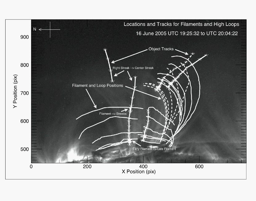
Figure 1:

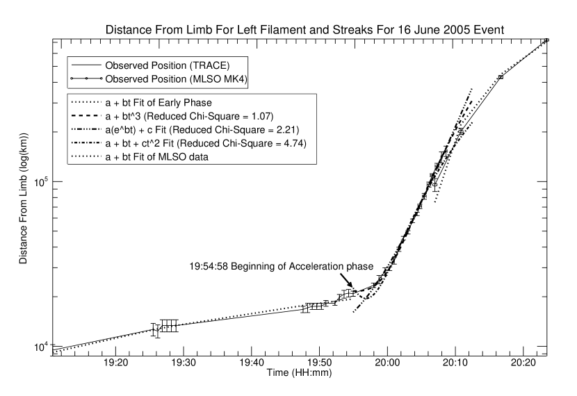
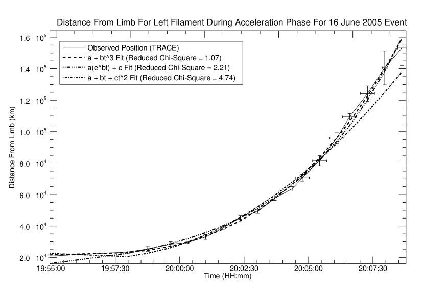
Figure 2:

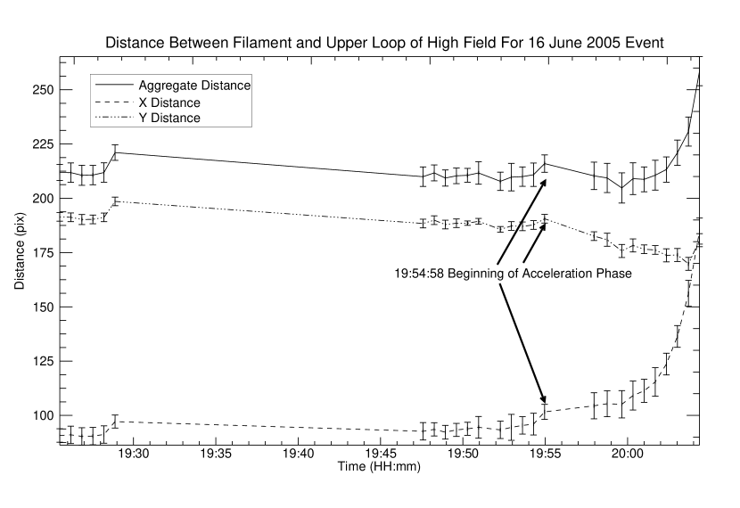
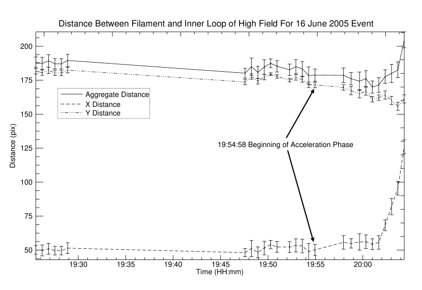
Figure 3:

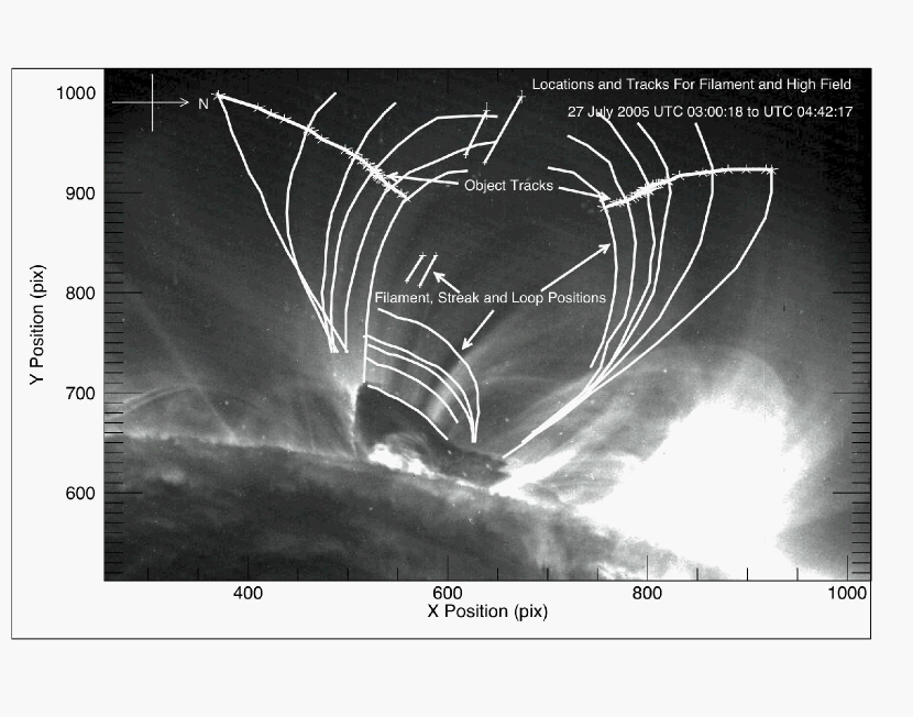
Figure 4:

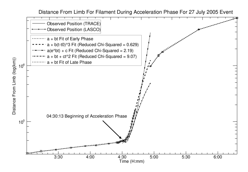
Figure 5:

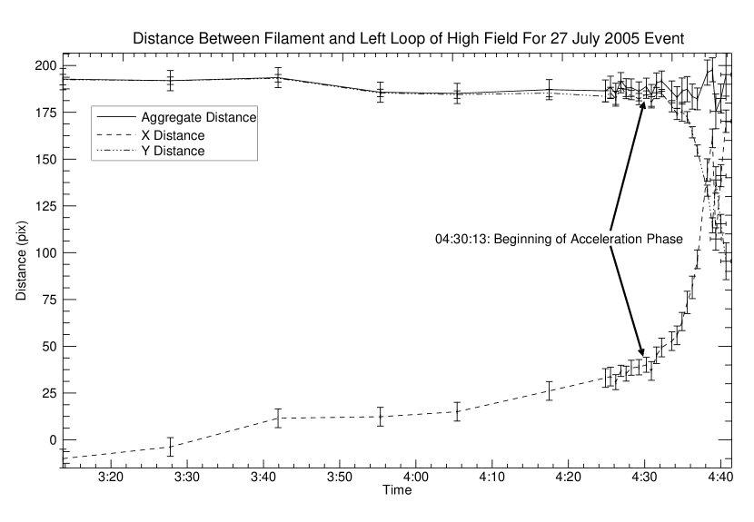
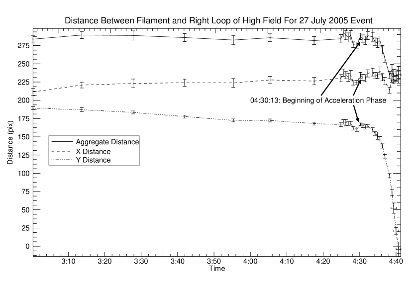
Figure 6:

Figure 7:

Figure 8:

Figure 9:

Figure 10:

Figure 11:

References

- Alexander et al. (2002) Alexander, D., Metcalf, T. R., & Nitta, N. V. 2002, Geophys. Res. Lett., 29, 41
- Bateman (1978) Bateman, G. 1978, MHD Instabilities, MIT, Cambridge, MA.
- Brueckner et al. (1995) Brueckner, G. E., Howard, R. A., Koomen, M. J., Korendyke, C. M., Michels, D. J., Moses, J. D., Socker, D. G., Dere, K. P., Lamy, P. L., Llebaria, A., Bout, M. V., Schwenn, R., Simnett, G. M., Bedford, D. K., & Eyles, C. J.: 1995, SPh 162, 357
- Chifor et al. (2006) Chifor, C., Mason, H. E., Tripathi, D., Isobe, H., & Asai, A. 2006, A&A, 458, 965
- Fan (2005) Fan, Y.: 2005, ApJ 630, 543
- Gallagher et al. (2003) Gallagher, P. T., Lawrence, G. R., & Dennis, B. R: 2003, ApJL 588, 53
- Gilbert et al. (2000) Gilbert, H. R., Holzer, T. E., Burkepile, J. T., & Hundhausen, A. J.: 2000, ApJ 537, 503
- Goff et al. (2005) Goff, C. P., van Driel-Gesztelyi, L., Harra, L. K., Matthews, S. A., & Mandrini, C. H.: 2005, A&A 434, 761
- Gopalswamy et al. (2003) Gopalswamy, N., Shimojo, M., Lu, W., Yashiro, S., Shibasaki, K., & Howard, R. A.: 2003, ApJ 586, 562
- Handy et al. (1999) Handy, B. N., Acton, L. W., Kankelborg, C. C., et al.: 1999, SPh 187, 229
- Hori et al. (2005) Hori, K., Ichimoto, K., Sakurai, T., Sano, I., & Nishino, Y.: 2005, ApJ 618, 1001
- Kahler et al. (1988) Kahler, S. W., Moore, R. L., Kane, S. R., & Zirin, H.: 1988, ApJ 328, 824
- Kliem and Török (2006) Kliem, B., & Török, T. 2006, Phys. Rev. Lett., 96, 255002
- Kliem et al. (2004) Kliem, B., Titov, V. S., & Török, T. 2004, A&A, 413, L23
- Kundu et al. (2004) Kundu, M. R., White, S. M., Garaimov, V. I., Manoharan, P. K., Subramanian, P., Ananthakrishnan, S., & Janardhan, P.: 2004, ApJ 607, 530
- Lynch et al. (2004) Lynch, B. J., Antiochos, S. K., MacNeice, P. J., Zurbuchen, T. H., & Fisk, L. A. 2004, ApJ, 617, 589
- Maričić et al. (2004) Maričić, D., Vršnak, B., Stanger, A. L., & Veronig, A. 2004, Sol. Phys., 225, 337
- Priest and Forbes (2002) Priest. E. R., & Forbes, T. G. 2002, A&A Rev., 10, 313
- Sterling and Moore (2004) Sterling, A. C. & Moore, R. L.: 2004, ApJ 613, 1221
- Sterling and Moore (2005) Sterling, A. C. & Moore, R. L.: 2005, ApJ 630, 1148
- Titov and Démoulin (1999) Titov, V. S., & Démoulin, P. 1999, A&A, 351, 707 (TD99)
- Török and Kliem (2005) Török, T. & Kliem, B.: 2005, ApJL 630, 97
- Török & Kliem (2007) Török, T., & Kliem, B. 2007, Astron. Nachr. 328, 743
- Török et al. (2004) Török, T., Kliem, B., & Titov, V. S. 2004, A&A, 413, L27
- van Tend and Kuperus (1978) van Tend, W., & Kuperus, M. 1978, Sol. Phys., 59, 115
- Vršnak (2001) Vršnak, B.: 2001, JGR 106, 25249
- Williams et al. (2005) Williams, D. R., Török, T., Démoulin, P., van Driel-Gesztelyi, L., & Kliem, B.: 2005, ApJL 628, 163
- Zhang and Golub (2003) Zhang, M. & Golub, L.: 2003, ApJ 595, 1251