Kähler potentials for the MSSM inflation and the spectral index

Abstract:

Recently it has been argued that some of the fine-tuning problems of the MSSM inflation associated with the existence of a saddle point along a flat direction may be solved naturally in a class of supergravity models. Here we extend the analysis and show that the constraints on the Kähler potentials in these models are considerably relaxed when the location of the saddle point is treated as a free variable. We also examine the effect of supergravity corrections on inflationary predictions and find that they can slightly alter the value of the spectral index. As an example, for flat direction field values $|\bar{\varphi}_{0}|=1\times 10^{-4}M_{P}$ we find $n\sim 0.92~{}...~{}0.94$ while the prediction of the MSSM inflation without any corrections is $n\sim 0.92$.

1 Introduction

Recently it has been argued that inflation can be realized already within the Minimally Supersymmetric Standard Model (MSSM) [1, 2]. In this case the inflaton field is a particular gauge invariant combination of squarks and sleptons corresponding to a flat direction of the MSSM. Its couplings to other MSSM degrees of freedom are thus fully determined and at least in principle measurable in laboratory experiments such as LHC or a future Linear Collider. This is in sharp contrast with the conventional models where the inflaton field is usually taken to be some ad hoc gauge singlet.

As discussed in [1], the phenomenologically acceptable candidates for the inflaton field are the dimension six flat directions udd and LLe. The potential along these flat directions can be written to leading order order as

$$V_{0}=\frac{1}{2}m^{2}|\phi|^{2}-\frac{A\lambda}{6}|\phi|^{6}+{\lambda}^{2}|\phi|^{10}\"{a},$$ (1)

where $|\phi|$ is the absolute value of the field parameterizing the flat direction. Here and elsewhere in the text we use units where $M_{P}\equiv 1$. The parameters $m$ and $A$ are supersymmetry (SUSY) breaking terms depending on the underlying supergravity (SUGRA) model and $\lambda$ is an effective coupling constant associated to the non-renormalizable operator lifting the flat direction.

For generic values of the SUSY breaking parameters, the potential Eq. (1) does not give rise to inflation. However, if one imposes the condition

$$A^{2}=40m^{2}\"{a},$$ (2)

the potential has a saddle point at

$$|\phi_{0}|=\Big{(}\frac{m}{\sqrt{10}\lambda}\Big{)}^{1/4}\ll 1\"{a}.$$ (3)

Close to the saddle point the potential becomes flat enough to support inflation and can be expanded as

$$V_{0}\approx\frac{4}{15}m^{2}|\phi_{0}|^{2}+\frac{16}{3}\frac{m^{2}}{|\phi_{0}|}(|\phi|-|\phi_{0}|)^{3}\"{a}.$$ (4)

If the initial conditions are such that $\phi\simeq\phi_{0}$, there follows a period of slow roll inflation with a very low scale $H_{\rm inf}\sim 1-10$ GeV producing primordial perturbations at the observed level and with the spectral index $n\simeq 0.92$ [1].

The success of the MSSM inflation obviously relies on the existence of the saddle point. Due to the exceptionally low inflationary scale, the potential needs to be extremely flat to produce large enough primordial perturbations. Consequently, the saddle point condition Eq. (2) must be satisfied with an accuracy of about $10^{-18}$ [2]. However, as proposed in [6] this apparent fine-tuning problem can be solved naturally in a class of supergravity models where the Kähler potential is chosen in such a manner that the saddle point condition Eq. (2) is identically satisfied. In [6] it was found that this can be achieved with Kähler potentials that up to quadratic part in $|\phi|$ have a fairly natural form encountered in various string theory compactifications but that also require fixing of some higher order terms. In this work we show that the constraints on the Kähler potentials are considerably relaxed if the location of the saddle point is treated as a free variable. In particular, we find that in order to identically produce the flat potential required by the MSSM inflation, the Kähler potential needs to be completely fixed only up to quadratic terms in $|\phi|$ and not to higher orders as in [6]. This considerably extends the class of allowed Kähler potentials and consequently increases the possibility to find theoretically motivated models that could yield the MSSM inflation.

We also discuss the effect of supergravity corrections on inflationary predictions. Although the corrections are suppressed by powers of $|\phi|$, they become significant in the vicinity of the saddle point Eq. (2) where the first and second derivative of the leading order potential Eq. (1) vanish. We find that in supergravity models where the MSSM inflation can be naturally realized, the relevant supergravity corrections to the inflaton potential will manifest themselves as additional linear terms in Eq. (4). This kind of corrections to the MSSM inflation have been discussed in [8, 9] (see also [10] for a discussion on dark matter and the MSSM inflation) without any particular supergravity motivation and it is well known that they can affect the spectral index and total number of e-foldings. The difference here is that since the corrections arise from a given supergravity model they are not arbitrary but can be exactly calculated.

We find that the supergravity corrections generically tend to increase the value of the spectral index. For the most typical field values [1] of the MSSM inflation $|\bar{\varphi}_{0}|\sim 10^{-4}$, where $|\bar{\varphi}_{0}|$ denotes value of the canonically normalized field at the saddle point, it is fairly easy to find Kähler potentials that bring the spectral index close to the observationally favoured value $n=0.948\pm 0.015$ [11]. For smaller field values, $|\bar{\varphi}_{0}|\lesssim 10^{-5}$ the corrections become negligible and one recovers the result $n\sim 0.92$ whereas large field values $|\bar{\varphi}_{0}|\gtrsim 10^{-3}$ typically yield too large spectral index. However it is still possible to choose the Kähler potential such that the resulting spectral index is consistent with observations even with large field values.

2 The supergravity models

In [6] it was found that the saddle point condition of the MSSM inflation can be satisfied identically in supergravity models with F-term supersymmmetry breaking and Kähler potentials of the form

$$K = \sum_{m}\beta_{m}{\rm ln}(h_{m}+h_{m}^{*})+\kappa\prod_{m}(h_{m}+h_{m}^{*})^{\alpha_{m}}|\phi|^{2}+\mu\Big{(}\kappa\prod_{m}(h_{m}+h_{m}^{*})^{\alpha_{m}}\Big{)}^{2}|\phi|^{4}+$$ (5)

$$\nu\Big{(}\kappa\prod_{m}(h_{m}+h_{m}^{*})^{\alpha_{m}}\Big{)}^{3}|\phi|^{6}+\mathcal{O}(|\phi|^{8}),\"{a}$$

where $h_{m}$ denote hidden sector fields and $\kappa,\beta_{m},\alpha_{m},\mu,\nu$ are constants. The superpotential is taken to be of the form

$$W=\hat{W}(h_{m})+\frac{\hat{\lambda}_{6}(h_{m})}{6}\phi^{6},$$ (6)

and the hidden sector dependent parts are treated as constants. The MSSM inflation is not a generic outcome of all such supergravity models, though, but one needs to place constraints on the parameters of the Kähler potential, see [6]. Moreover, the hidden sector or moduli fields $h_{m}$ need to be stabilized before the beginning of inflation by some mechanism not consistently taken into account here.

It turns out that the fairly strict constraints on the Kähler potentials found in [6] can be considerably relaxed by allowing the location of the saddle point $|\phi_{0}|$ to slightly vary from the value given by Eq. (2). This is indeed a natural thing to do since Eq. (2) results from the leading order part of the inflaton potential alone while supergravity models typically yield higher order corrections as well. Therefore we write $|\phi_{0}|$ as an expansion

$$|\phi_{0}|^{4}=\bar{|\phi_{0}|}^{4}(1+\Delta_{1}|\phi_{0}|+\Delta_{2}|\phi_{0}|+...)\"{a},$$ (7)

where $\bar{|\phi_{0}|}$ denotes the leading order part determined by Eq. (2) and the terms $\Delta_{n}|\phi_{0}|\sim\mathcal{O}(\bar{|\phi_{0}|}^{2n})$ represent yet unfixed higher order degrees of freedom corresponding to the higher order terms in the potential.

Using Eq. (7) and repeating the analysis of [6] one finds that the flat potential of the MSSM inflation is identically obtained if the parameters in the Kähler potential Eq. (5) are chosen according to Table $(1)$.

Table 1: The constraints on the parameters of the Kähler potential Eq. $(2.1)$ implied by the flatness of the inflaton potential.

$\rule{0.0pt}{12.91663pt}\beta=\sum\beta_{m}$	$\alpha=\sum\alpha_{m}$	$\gamma=\sum\frac{\alpha_{m}^{2}}{\beta_{m}}$	$\delta=\sum\frac{\alpha_{m}^{3}}{\beta_{m}^{2}}$
$\rule{0.0pt}{12.91663pt}-7$	$~{}~{}0$	$\frac{1}{4}-3\mu$	$\delta$
$\rule{0.0pt}{12.91663pt}-7$	$-\frac{25}{9}$	$-\frac{46}{81}-\frac{22}{9}\mu$	$-\frac{2414}{16767}-\frac{628}{1863}\mu-\frac{2804}{207}\mu^{2}+\frac{162}{23}\nu$
$\rule{0.0pt}{12.91663pt}-11$	$-\frac{1}{9}$	$\frac{28}{81}-\frac{26}{9}\mu$	$\frac{6556}{69255}-\frac{3736}{7695}\mu-\frac{12596}{855}\mu^{2}+\frac{162}{19}\nu$
$\rule{0.0pt}{12.91663pt}-11$	$-4$	$-\frac{7}{8}-\frac{5}{2}\mu$	$-\frac{339}{1600}-\frac{73}{200}\mu-\frac{1371}{100}\mu^{2}+\frac{36}{5}\nu$

The conditions in Table $(1)$ are much less restrictive than those found in [6]. In particular, the parameters $\mu$ and $\nu$ determining the form of the Kähler potential are not fixed which considerably extends the class of allowed Kähler potentials. They can not be chosen completely at will however, since one needs to see to that real solutions for the conditions on $\alpha_{m}$ and $\beta_{m}$ in Table $(1)$ exist. A necessary condition for this is to require $|\delta|\leq|\gamma|^{3/2}$, assuming $\beta_{m}$’s to be negative integers as suggested by the string theory motivated models. Moreover, the parameters $\mu$ have to be chosen such that $\gamma<0$.

It is quite interesting to notice that the class of Kähler potentials defined by Eq. (5) and Table $(1)$ includes for example the simple logarithmic form

$$K=-{\rm ln}\Big{(}\prod_{m}(h_{m}+h_{m}^{*})^{-\beta_{m}}-\kappa\prod_{m}(h_{m}+h_{m}^{*})^{\alpha_{m}-\beta_{m}}|\phi|^{2}\Big{)}\"{a},$$ (8)

where the parameters are now subject to the constraints in Table $(2)$.

Table 2: The constraints on the parameters of the Kähler potential Eq. $(2.2)$ implied by the flatness of the inflaton potential.

$\beta=\sum\beta_{m}$	$\alpha=\sum\alpha_{m}$	$\gamma=\sum\frac{\alpha_{m}^{2}}{\beta_{m}}$	$\delta=\sum\frac{\alpha_{m}^{3}}{\beta_{m}^{2}}$
$-7$	$~{}~{}0$	$-\frac{5}{4}$	$\delta$
$-7$	$-\frac{25}{9}$	$-\frac{145}{81}$	$-\frac{985}{729}$
$-11$	$-\frac{1}{9}$	$-\frac{89}{81}$	$-\frac{721}{729}$
$-11$	$-4$	$-\frac{17}{8}$	$-\frac{91}{64}$

One can check that solutions for these constraints do exist. As an example, in the case $\beta=7$, $\alpha=0$ the constraints in Table $(2)$ are satisfied for a choice

$$\beta_{m}=-1,~{}\alpha_{1}=1,~{}\alpha_{2}=\alpha_{3}=\alpha_{4}=\alpha_{5}=-\frac{1}{4},~{}\alpha_{6}=\alpha_{7}=0\"{a}.$$ (9)

Both the logarithmic Kähler potentials Eq. (8) and the more generic forms Eq. (5) bear some resemblance to the results appearing in various string theory compactifications. Up to the quadratic part, the form of Eq. (8) is encountered e.g. in Abelian orbifold compactifications of the heterotic string theory [12] and in intersecting D-brane models [13]. Logarithmic Kähler potentials on the other hand are obtained e.g. in large radius limit of Calabi-Yau compactifications and also in no-scale supergravity models [14] although the results are not precisely of the form given in Eq. (8). However, it is interesting even in its own rights that the saddle point condition of the MSSM inflation is satisfied to the required extraordinary precision with Kähler potentials Eq. (8) that can be expressed in terms of a single natural function.

3 The supergravity corrections to inflation

The field $\phi$ parameterizing the flat direction has a non-canonical kinetic term due to the form of the Kähler potentials Eq. (5). Instead of using $\phi$ we therefore switch to the canonically normalized field

$$\varphi\equiv(\kappa\prod_{m}(h_{m}+h_{m}^{*})^{\alpha_{m}})^{1/2}\phi~{}(1+\mathcal{O}(|\phi|^{2}))\equiv\hat{Z}_{2}^{1/2}\phi~{}(1+\mathcal{O}(|\phi|^{2}))\"{a},$$ (10)

that will be interpreted as the inflaton. Provided the conditions in Table $(1)$ are satisfied, the inflaton potential in the supergravity models described above identically becomes [6]

$$V(|\varphi|)=\frac{4}{15}m_{\varphi}^{2}|\bar{\varphi}_{0}|^{2}+\frac{16}{3}\frac{m_{\varphi}^{2}}{|\bar{\varphi}_{0}|}(|\varphi|-|\bar{\varphi}_{0}|)^{3}+\xi m_{\varphi}^{2}|\bar{\varphi}_{0}|^{7}(|\varphi|-|\bar{\varphi}_{0}|)+\ldots\"{a},$$ (11)

in the vicinity of the point

$$|\bar{\varphi}_{0}|\equiv\hat{Z}_{2}^{1/2}|\bar{\phi}_{0}|\equiv\Big{(}\frac{m_{\varphi}}{\sqrt{10}\lambda_{\varphi}}\Big{)}^{1/4}\"{a}.$$ (12)

Here $m_{\varphi}=m\hat{Z}_{2}^{~{}-1/2},\lambda_{\varphi}=\lambda\hat{Z}_{2}^{~{}-5/2}$ and the explicit expressions for them are given in the Appendix. The first two terms in Eq. (11) arise from the leading order part of the supergravity scalar potential and, due to the constraints in Table $(1)$, the lowest order non-vanishing supergravity correction is of the form $\xi m_{\varphi}^{2}|\bar{\varphi}_{0}|^{7}(|\varphi|-|\bar{\varphi}_{0}|)$ and it is small enough not to spoil the flatness of the potential [6]. The coefficient $\xi$ is determined by the $o(|\phi|^{8})$ part of the Kähler potential.

Although the small supergravity correction $\xi m_{\varphi}^{2}|\bar{\varphi}_{0}|^{7}(|\varphi|-|\bar{\varphi}_{0}|)$ does not invalidate the success of the MSSM inflation, it may still be significant at the early stages of the inflationary period where the slope arising from the leading order potential is very small. Indeed, small linear corrections like this have been considered without any particular supergravity motivation in [8, 9] and it has been shown that they will affect the resulting spectral index. The difference in our analysis is that the corrections are not arbitrary but arise from the supergravity model and are thus completely specified. In the particular supergravity models considered here, the linear term in Eq. (11) is also the only relevant correction to the leading order potential since the higher order supergravity corrections are too small to leave any observable imprints [6].

The inflationary properties of the potential Eq. (11) can be straightforwardly analyzed [8, 9] using the standard slow-roll approximation. If the field starts at rest close to $|\bar{\varphi}_{0}|$, there follows a period of inflation with the amplitude of curvature perturbation given by

$$\mathcal{P}_{\mathcal{R}}^{1/2} \approx \frac{4}{45\sqrt{5}\pi}\frac{m_{\varphi}}{\xi|\bar{\varphi}_{0}|^{4}}\Big{[}1+{\rm tan}^{2}\Big{(}{\rm arctan}\big{(}\frac{1}{30\sqrt{\xi}|\bar{\varphi}_{0}|}\big{)}-15\sqrt{\xi}|\bar{\varphi}_{0}|N_{*}\Big{)}\Big{]}^{-1}$$

$$\approx \mathcal{P}_{\mathcal{R}}^{1/2}(\xi=0)\Big{(}1-75N^{2}_{*}\xi|\bar{\varphi}_{0}|^{2}+\mathcal{O}(\xi^{2}|\bar{\varphi}_{0}|^{4})\Big{)}\"{a},$$

and the spectral index by

$$n \approx 1-60\sqrt{\xi}|\bar{\varphi}_{0}|{\rm tan}\Big{(}{\rm arctan}\big{(}\frac{1}{30\sqrt{\xi}|\bar{\varphi}_{0}|}\big{)}-15\sqrt{\xi}|\bar{\varphi}_{0}|N_{*}\Big{)}$$

$$\approx n(\xi=0)+300N_{*}\xi|\bar{\varphi}_{0}|^{2}+\mathcal{O}(\xi^{2}|\bar{\varphi}_{0}|^{4})\"{a}\"{a}.$$

By taking $\xi=0$ one recovers the results of [1] for the MSSM inflation without any corrections. Here $N_{*}\sim 50$ is the number of e-foldings after the observable scales exit the horizon and we have assumed that the end of inflation is determined by

$$|\eta|=\Big{|}\frac{V^{\prime\prime}}{V}\Big{|}\sim 1~{}~{}\Longrightarrow~{}~{}\frac{|\bar{\varphi}_{0}|-|\varphi_{\rm end}|}{|\bar{\varphi}_{0}|^{3}}\approx\frac{1}{120}\"{a}.$$ (15)

The magnitude of the supergravity corrections in Eqs. (3), (3) is determined by the term $\xi|\bar{\varphi}_{0}|^{2}$ and assuming $N_{*}\sim 50$ they become significant for $\sqrt{\xi}|\bar{\varphi}_{0}|\gtrsim 8\times 10^{-4}$. In the supergravity models considered here one finds $|\xi|\lesssim\mathcal{O}(100)$ and for the field values $|\bar{\varphi}_{0}|\sim 10^{-4}$ typical in the MSSM inflation [1, 2], the corrections can thus become important. On the other hand, the corrections can always be made negligible by taking the field values to be small enough $|\bar{\varphi}_{0}|\lesssim 10^{-5}$, which corresponds to $|\lambda_{\varphi}|\gg 1$ in Eq. (12). In this limit the results of [1, 2] are thus recovered.

If the soft mass $m_{\varphi}$ is regarded as an adjustable parameter, the supergravity corrections can be seen as modifications of the spectral index alone. This is because the amplitude of perturbations Eq. (3) depends explicitly on $m_{\varphi}$ while the spectral Eq. (3) index does not. By slightly changing the value of $m_{\varphi}$, the amplitude can thus be kept fixed while varying the spectral index. However, besides the spectral index, the supergravity corrections also affect the total number of e-foldings tending to make the inflationary period shorter for $\xi>0$ [8, 9]. For $\xi>0$ the total number of e-foldings is given by

$$N_{\rm tot}\approx\frac{1}{15\sqrt{\xi}|\bar{\varphi}_{0}|}\Big{(}{\rm arctan}\Big{(}\frac{1}{30\sqrt{\xi}|\bar{\varphi}_{0}|}\Big{)}-{\rm arctan}\Big{(}\frac{4}{\sqrt{\xi}}\frac{|\bar{\varphi}_{0}|-|\varphi_{\rm in}|}{|\bar{\varphi}_{0}|^{4}}\Big{)}\Big{)}\"{a},$$ (16)

which becomes strongly dependent on the initial value of the field $|\varphi_{\rm in}|$ when the supergravity corrections get large and, unlike in the $\xi=0$ case, the initial conditions can not be explained by a period of eternal inflation even in principle since the classical force always overcomes the quantum effects for $|\xi|\gtrsim 10^{-1}|\lambda_{\varphi}|$. Requiring sufficiently long period of inflation $N_{\rm tot}\gtrsim 50$, Eq. (16) yields an absolute upper bound $\sqrt{\xi}|\bar{\varphi}_{0}|\lesssim 3\times 10^{-3}$ for the allowed magnitude of supergravity corrections and using Eq. (3) this implies $n\lesssim 1$ [9]. In the next Section we show that the parameters in the Kähler potentials Eq. (5) can easily be chosen such that this condition is satisfied.

4 The spectral index

As a simple example we first discuss the supergravity corrections that arise from the logarithmic Kähler potentials defined by Eq. (8) and Table $(2)$. In this case the supergravity corrections and in particular the parameter $\xi$ in Eq. (11) are completely determined since the Kähler potential is known to all orders in $|\phi|$. Using standard supergravity formulae it is then straightforward to work out the explicit expressions for $\xi$ in each of the cases of Table $(2)$, see the Appendix. The results are shown in Table $(3)$.

Table 3: The coefficient $\xi$ of the lowest order non-vanishing supergravity corrections arising from the Kähler potentials defined by Eq. (2.4) and Table $(2)$. Here $\epsilon\equiv\sum\alpha_{m}^{4}/\beta_{m}^{3}$ and for simplicity we have given the expressions for $\xi$ to the precision of two digits.

$\beta=\sum\beta_{m}$	$\alpha=\sum\alpha_{m}$	$\gamma=\sum\frac{\alpha_{m}^{2}}{\beta_{m}}$	$\delta=\sum\frac{\alpha_{m}^{3}}{\beta_{m}^{2}}$	$\xi$
$-7$	$~{}~{}0$	$-\frac{5}{4}$	$\delta$	$0$
$-7$	$-\frac{25}{9}$	$-\frac{145}{81}$	$-\frac{985}{729}$	$-7\times(1.16+\epsilon)$
$-11$	$-\frac{1}{9}$	$-\frac{89}{81}$	$-\frac{721}{729}$	$-0.25\times(1.00+\epsilon)$
$-11$	$-4$	$-\frac{17}{8}$	$-\frac{91}{64}$	$-4.8\times(1.16+\epsilon)$

Assuming $\beta_{m}$ to be negative integers, the constraints in Table $(2)$ imply $\epsilon\equiv\sum\alpha_{m}^{4}/\beta_{m}^{3}\sim-1$ which yields an estimate $|\xi|\lesssim 1$. As discussed above, the supergravity corrections to the spectral index Eq. (3) become significant for $\sqrt{\xi}|\bar{\varphi}_{0}|\gtrsim 8\times 10^{-4}$ and for $|\xi|\lesssim 1$ this requires $|\bar{\varphi}_{0}|\gtrsim 10^{-3}$. For the typical field values of the MSSM inflation $|\bar{\varphi}_{0}|\sim 10^{-4}$ the corrections are thus negligible and we recover the standard result $n\sim 0.92$ for the spectral index of the MSSM inflation. In the case $\beta=-7$ and $\alpha=0$ of Table $(2)$ this actually holds for any field values since the coefficient $\xi$ vanishes identically.

To discuss the supergravity corrections with the more generic Kähler potentials defined by Eq. (5) and Table $(1)$, we first need to determine the potential up to $|\phi|^{8}$. The most natural extension of Eq. (5) is to write

$$K = \sum_{m}\beta_{m}{\rm ln}(h_{m}+h_{m}^{*})+\kappa\prod_{m}(h_{m}+h_{m}^{*})^{\alpha_{m}}|\phi|^{2}+\mu\Big{(}\kappa\prod_{m}(h_{m}+h_{m}^{*})^{\alpha_{m}}\Big{)}^{2}|\phi|^{4}+$$ (17)

$$\nu\Big{(}\kappa\prod_{m}(h_{m}+h_{m}^{*})^{\alpha_{m}}\Big{)}^{3}|\phi|^{6}+\rho\Big{(}\kappa\prod_{m}(h_{m}+h_{m}^{*})^{\alpha_{m}}\Big{)}^{4}|\phi|^{8}+\mathcal{O}(|\phi|^{10})\"{a},$$

where $\rho$ is a free constant. The coefficient $\xi$ can again be straightforwardly computed in the different cases of Table $(1)$ and the result will be of the form $\xi=\xi(\mu,\nu\rho,\epsilon)$, where $\epsilon\equiv\sum\alpha_{m}^{4}/\beta_{m}^{3}$. The explicit expressions are given in the Appendix and by substituting them into Eq. (3) one readily finds the resulting spectral index.

Just like with the simple logarithmic Kähler potentials discussed above, $\xi$ vanishes identically in the case $\beta=-7,~{}\alpha=0$ of Table $(1)$ and in this particular case the supergravity corrections are thus absent. However, the situation is more complicated in the other cases of Table $(1)$ as can be seen in Fig. $(1)$ below.

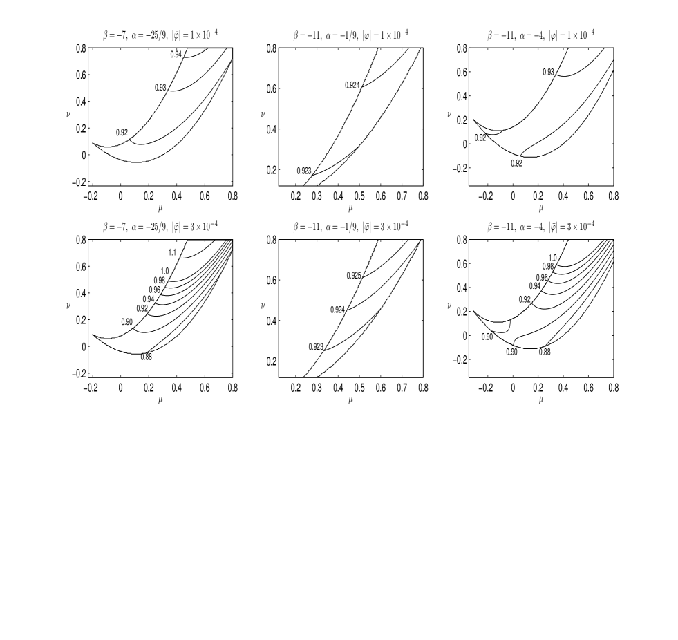
Figure 1: The values of the spectral index in the different cases of Table $(1)$. The case $\beta=-7,\alpha=0$ is trivial with $n=0.923$ and is thus not included. The curves with labels denote countour lines while the boundary curves describe the region where the necessary conditions for the existence of solutions for Table $(1)$ are satisfied. Here the parameters $\rho$ and $\epsilon$ in the Kähler potential Eq. (4.1) are chosen as $\rho=1/4$, $\epsilon=\gamma^{2}$.

There the dependence of the spectral index Eq. (3) on the parameters of the Kähler potential Eq. (17) is illustrated for different field values $|\bar{\varphi}_{0}|$. In Fig. $(1)$ we have shown only the values of $\mu$ and $\nu$ for which the necessary conditions for the existence of solutions for the constraints in Table $(1)$, discussed in Section 2, are satisfied. We have also fixed the parameters $\epsilon$ and $\rho$ appearing in the expression of $\xi$, but changing their values will not significantly alter the qualitative behaviour of the spectral index.

Fig. $(1)$ clearly shows that the supergravity corrections typically tend to bring the spectral index above the value $n\sim 0.92$ that corresponds to the MSSM inflation without any corrections. In the case $\beta=-11,~{}\alpha=-1/9$ of Table $(1)$ the corrections are very small for all reasonable field values and we effectively recover the value $n\sim 0.92$ like in the case $\beta=-7,~{}\alpha=0$. In the other cases of Table $(1)$, the corrections are larger and the range of possible values of the spectral index is highly dependent on the field value $|\bar{\varphi}_{0}|$. For a typical choice $|\bar{\varphi}_{0}|=1\times 10^{-4}$ shown in the upper panel of Fig. $(1)$ the spectral index depends rather weakly on the parameters $\mu$ and $\nu$ of the Kähler potential and in the region shown in Fig. $(1)$ we find $n\sim 0.92~{}...~{}0.94$. For larger field values the corrections rapidly become larger and the parameters $\mu$ and $\nu$ need to be chosen more carefully in order to obtain a spectral index consistent with observations. This is demonstrated in the lower panel of Fig. $(1)$ for $|\bar{\varphi}_{0}|=3\times 10^{-4}$. On the other hand, as discussed in Section 3, for small enough field values $|\bar{\varphi}_{0}|\lesssim 10^{-5}$ the supergravity corrections become negligible and we recover $n\sim 0.92$ in all the cases of Table $(1)$.

5 Conclusions

In this work we have discussed the supergravity origin of the MSSM inflation [1, 2] extending the analysis of [6]. We have shown that the MSSM inflation can be realized in supergravity models with Kähler potentials of the simple form

$$K = \sum_{m}\beta_{m}{\rm ln}(h_{m}+h_{m}^{*})+\kappa\prod_{m}(h_{m}+h_{m}^{*})^{\alpha_{m}}|\phi|^{2}+\mu\Big{(}\kappa\prod_{m}(h_{m}+h_{m}^{*})^{\alpha_{m}}\Big{)}^{2}|\phi|^{4}+$$ (18)

$$\nu\Big{(}\kappa\prod_{m}(h_{m}+h_{m}^{*})^{\alpha_{m}}\Big{)}^{3}|\phi|^{6}+\mathcal{O}(|\phi|^{8}),\"{a}$$

that at least up to the quadratic part closely resemble the results found in various string theory compactifications [12, 13]. The flatness of the inflaton potential is a natural outcome of such supergravity models provided the parameters $\beta_{m}$ and $\alpha_{m}$ in the Kähler potential are appropriately chosen, see Table $(1)$ in the text. However, unlike in the result found in [6], we have shown that it is not necessary to completely fix the coefficients $\mu$ and $\nu$. This considerably extends the class of allowed Kähler potentials and thus increases the possibility to find realistic supergravity models that would yield the MSSM inflation. We wish to emphasize though that in considering the MSSM inflation [1, 2] driven by a single degree of freedom, we are implicitly assuming the moduli fields of the supergravity model to be stabilized by some mechanism before the beginning of inflation. This represents a non-trivial assumption and should be discussed separately in the context of any realistic model to make the analysis complete [7].

We have also examined the possibility that the underlying supergravity model would not yield exactly the MSSM inflation proposed in [1, 2] but a slightly modified model of the type [8, 9]. In this case the supergravity corrections cause small deviations from the saddle point condition of the MSSM inflation and thus affect the inflationary predictions, mainly the spectral index. The magnitude of the corrections depends both on the parameters in the Kähler potential and on the field value $|\bar{\varphi}_{0}|$ but they typically tend to bring the spectral index above the value $n\sim 0.92$ that corresponds to the MSSM inflation without any corrections [1, 2]. As an example, for a natural choice $|\bar{\varphi}_{0}|=1\times 10^{-4}$ one finds $n\sim 0.92~{}...~{}0.94$ if the coefficients $\mu$ and $\nu$ in the Kähler potential are taken to be less than unity. The range of possible values becomes larger for larger field values but it is still possible to choose the Kähler potential such that the spectral index is consistent with observations. If the field values are small enough $|\bar{\varphi}_{0}|\lesssim 10^{-5}$ the corrections become negligible and we always recover the result $n\sim 0.92$.

The results obtained here and in [6] suggest that it might be possible to realize the MSSM inflation naturally in reasonable supergravity models. The Kähler potential certainly needs to be chosen in specific manner but there is no need for excessive fine-tuning. The slightly too small spectral index of the original model of the MSSM inflation [1, 2] may also be easily cured as discussed above. It would be an interesting subject of future research to see if these conclusions will change when the stabilization of the moduli fields and the radiative corrections are properly taken into account.

Appendix A The supergravity scalar potential

The supergravity scalar potential is written as

$$V=e^{K}|W|^{2}\Big{(}K^{M{\bar{N}}}(K_{M}K_{{\bar{N}}}+\frac{W_{M}W^{*}_{{\bar{N}}}}{|W|^{2}}+K_{M}\frac{W^{*}_{{\bar{N}}}}{W^{*}}+K_{{\bar{N}}}\frac{W_{M}}{W})-3\Big{)}\"{a},$$ (19)

where $K^{M{\bar{N}}}$ is the inverse of the Kähler metric $K_{M{\bar{N}}}$, and the lower indices denote derivatives with respect to fields. The potential for the flat direction $\phi$ is found by substituting the Kähler and superpotentials, given by Eqs. (17) and (6) respectively, into Eq. (19).

If the conditions in Table $(1)$ are satisfied and the hidden sector dependent parts of the superpotential are treated as constants, the potential can be expanded as in Eq. (11) and the explicit expressions for $m_{\varphi}$, $\lambda_{\varphi}$ in Eqs. (11), (12) read

$$m^{2}_{\varphi} = 2e^{\hat{K}}|\hat{W}|^{2}(\alpha-\beta-2)$$ (20)

$$\lambda_{\varphi} = e^{\hat{K}/2}\hat{Z_{2}}^{-3}|\hat{\lambda}_{6}|\"{a},$$ (21)

where we have denoted

$$\hat{K} \equiv \sum_{m}\beta_{m}{\rm ln}(h_{m}+h_{m}^{*})$$ (23)

$$\hat{Z}_{2} \equiv \kappa\prod_{m}(h_{m}+h_{m}^{*})^{\alpha_{m}}\"{a}.$$ (24)

The coefficients $\xi$ in Eq. (11) in the four different cases of Table $(1)$ are given by

$$\xi_{1} = 0$$ (25)

$$\xi_{2} = -\frac{328637}{1509030}-\frac{26674}{3105}\mu^{2}-\frac{631648}{1035}\mu^{3}+\frac{376}{69}\nu$$

$$+\mu(-\frac{1154}{1215}+\frac{12864}{23}\nu)-96\rho-7\epsilon$$

$$\xi_{3} = \frac{370583}{62329500}-\frac{21457}{64125}\mu^{2}-\frac{491524}{21375}\mu^{3}+\frac{484}{1425}\nu$$

$$+\mu(-\frac{25921}{577125}+\frac{10434}{475}\nu)-\frac{21}{5}\rho-\frac{1}{4}\epsilon$$

$$\xi_{4} = -\frac{8649}{40000}-\frac{15483}{2500}\mu^{2}-\frac{263647}{625}\mu^{3}+\frac{516}{125}\nu$$ (28)

$$+\mu(-\frac{6909}{10000}+\frac{48528}{125}\nu)-\frac{336}{5}\rho-\frac{24}{5}\epsilon$$

where the subindices refer to the rows of Table $(1)$.

References

- [1] R. Allahverdi, K. Enqvist, J. Garcia-Bellido, and A. Mazumdar, Phys. Rev. Lett. 97:191304, 2006 [arXiv:hep-ph/0605035].
- [2] R. Allahverdi, K. Enqvist, J. Garcia-Bellido, A. Jokinen, and A. Mazumdar, arXiv:hep-ph/0610134.
- [3] M. Dine, L. Randall and S. Thomas, Phys. Rev. Lett.75:398, 1995 [arXiv:hep-ph/9503303]; Nucl.Phys.B458:291, 1996 [arXiv:hep-ph/9507453].
- [4] T. Gherghetta, C. F. Kolda and S. P. Martin, Nucl.äPhys.äB 468:37, 1996 [arXiv:hep-ph/9510370].
- [5] K. Enqvist and A. Mazumdar, Phys. Rept. 380:99, 2003 [arXiv:hep-ph/0209244].
- [6] K. Enqvist, L. Mether and S. Nurmi, [arXiv:0706.2355].
- [7] Z. Lalak and K. Turzynski, arXiv:0710.0613 [hep-th].
- [8] J. C. Bueno Sanchez, D. Lyth and K. Dimopoulos, JCAP 0701:015, 2007 [arXiv:hep-ph/0608299].
- [9] R. Allahverdi and A. Mazumdar, arXiv:hep-ph/0610069.
- [10] R. Allahverdi, B. Dutta and A. Mazumdar, Phys.äRev.ä D 75 (2007) 075018 [arXiv:hep-ph/0702112].
- [11] D. N. Spergel et al. [WMAP Collaboration], arXiv:astro-ph/0603449.
- [12] See e.g. L. E. Ibanez and D. Lust, Nucl.äPhys.ä B 382, 305 (1992) [arXiv:hep-th/9202046] and references therein.
- [13] See e.g. D. Lust, S. Reffert and S. Stieberger, Nucl.äPhys.ä B 727 (2005) 264 [arXiv:hep-th/0410074] and references therein.
- [14] For a review of no-scale models, see A. B. Lahanas and D. N. Nanopoulos, Phys. Rept. 145:1, 1987.
- [15] R. Allahverdi, A. R. Frey and A. Mazumdar, Phys.äRev.ä D 76 (2007) 026001 [arXiv:hep-th/0701233].