Spatial confinement effects on quantum field theory using nonlinear coherent states approach

Abstract

We study some basic quantum confinement effects through investigation a deformed harmonic oscillator algebra. We show that spatial confinement effects on a quantum harmonic oscillator can be represented by a deformation function within the framework of nonlinear coherent states theory. Using the deformed algebra, we construct a quantum field theory in confined space. In particular, we find that the confinement influences on some physical properties of the electromagnetic field and it gives rise to nonlinear interaction. Furthermore, we propose a physical scheme to generate the nonlinear coherent states associated with the electromagnetic field in a confined region.

1 Introduction

The physical size and shape of the materials strongly effect the nature, the dynamics of the electronic excitations, the lattice vibrations, and the dynamics of carriers. For example, in the mesoscopic systems, the dimension of system is comparable with the coherence length of carriers and this leads to some new phenomena that they do not appear in a bulk semiconductor, such as quantum interference between carrier’s motion [1]. In these physical systems different particles are confined in a small space and interact with each other. As usual, we use quantum field theory (QFT) and second quantization procedure for considering interacting many particles physical systems. Standard QFT is based on quantum mechanics on an infinite line without any boundaries. However, the presence of infinite walls in standard QFT can detect vacuum effect of electromagnetic field and gives rise to Casimir effect [2]. Hence, in a system with small dimensions we expect some new phenomena appear, and barriers effects show themselves.
Recent progress in growth techniques and development of micromachinig technology in designing mesoscopic systems and nanostructures, have led to intensive theoretical [3] and experimental investigations [4] on electronic and optical properties of those systems. The most important point about the nanoscale structures is that the quantum confinement effects play the center-stone role. One can even say in general that recent success in nanofabrication technique has resulted in great interest in various artificial physical systems with usual phenomena driven by the quantum confinement (quantum dots, quantum wires and quantum wells). A number of recent experiments have demonstrated that isolated semiconductor quantum dots are capable of emitting light [5]. It becomes possible to combine high-Q optical microcavities with quantum dot emitters as the active medium [6]. Furthermore, there are many theoretical attempts for understanding the optical and electronic properties of nanostructures especially semiconductor quantum dots [7]. Because of intensive researches in this area, it is reasonable to consider the finite size effects on the EM field including the quantization of the EM field in confined regions that their sizes are of order of electromagnetic wavelength, such as microcavities. On the other hand, a nanostructure such as quantum dot, is a system that carrier’s motion is confined inside a small region, and during the interaction with other systems, the generated excitations such as phonons, excitons, plasmons are confined in small region. Hence we want to answer this question: what are the spatial confinement effects on excitation states in quantum field theoretical description of nanostructures? It seems that to answer this question we need to know the confinement and boundary conditions effects in QFT. First, we consider spatial confinement effect on a simple quantum harmonic oscillator and then we shall use this oscillator in quantizing the fields.
As mentioned before, the standard QFT is based on the quantum mechanics on an infinite line. In the canonical QFT the main tool is quantum oscillator. Energy eigenvalues of quantum harmonic oscillator (QHO) is given by $E_{n}=(n+\frac{1}{2})\hbar\omega$, and these successive energy levels were interpreted as being obtained by creation of a quantum particle of energy $\hbar\omega$. This interpretation of the energy spectrum of QHO was successfully used in the second quantization formalism [8]. Plank’s hypothesis is realized in the second quantization formalism by using creation and annihilation operators of the QHO. This realization is obtained for QHO defined on an infinite line.
It is reasonable to claim that, in considering QFT in a finite region one can use energy levels of a QHO confined in that finite space and therefore analyze the consequences of this assumption in construction of such QFT on a compact manifold. As we shall see in subsequent sections, the spatial confinement of the QHO leads to a deformed Heisenberg algebra for the ordinary harmonic oscillator. A deformed algebra is a nontrivial generalization of a given algebra through the introduction of one or more complex parameters, such that, in a certain limit of parameters the non-deformed algebra is recovered; these parameters are called deformation parameters. There have been several attempts to generalize Heisenberg algebra, and a particular deformation of Heisenberg algebra has led to the notion f-oscillator [9]. An f-oscillator is a non-harmonic system, that from mathematical point of view its dynamical variables (creation and annihilation operators) constructed from a non canonical transformation through

$$\hat{A}=\hat{a}f(\hat{n})\hskip 28.45274pt,\hskip 28.45274pt\hat{A}^{{\dagger}}=f(\hat{n})\hat{a}^{{\dagger}},$$ (1)

where $\hat{a}$ and $\hat{a}^{{\dagger}}$ are corresponding harmonic oscillator operators and $\hat{n}=\hat{a}^{{\dagger}}\hat{a}$. The function $f(\hat{n})$ is called deformation function that depends on the number of quanta and some physical parameters. The presence of operator-valued deformation function causes the Heisenberg algebra of the standard QHO to transform into a deformed Heisenberg algebra. The nonlinearity in f-oscillators means dependence of the frequency on the intensity [10]. On the other hand, in contrast to the standard QHO, f-oscillators have not equal spaced energy spectrum. If we confine a simple QHO inside an infinite well, due to the spatial confinement, the energy levels constitute a spectrum that is not equal spaced. Therefore, in this case it is reasonable to expect to find a corresponding f-oscillator. One of the most interesting features of the QHO is the construction of coherent states, as the eigenfunction of annihilation operator. As is well known [9] one can introduce Nonlinear coherent states or f-coherent states as the right-hand eigenstates of deformed annihilation operator $\hat{A}$. It has been shown that these families of generalized coherent states exhibit various non-classical properties [11]. Due to these properties and their applications, generation of these states is a very important issue in the context of quantum optics. The f-coherent states may appear as stationary states of the center-of-mass motion of a trapped ion [12]. Furthermore, a theoretical scheme for generation of these states in micromaser in the frame work of intensity-dependent Jaynes-Cummings model has been proposed [13].
It has also been shown [14] that there is a close connection between the deformation function appeared in the nonlinear coherent states algebraic structure and the non-commutative geometry of the configuration space. Furthermore, it has been shown recently [15], that if a two-mode QHO confined on the surface of a sphere, can be interpreted as a single mode deformed oscillator, whose and its quantum statistics depends on the curvature of sphere.
Motivated by the above-mentioned results, in the present contribution we are intended to investigate the spatial confinement effects on physical properties of a standard QHO. It will be seen that the confinement leads to deformation of standard QHO. Then we use this confined oscillator to considering boundary effects in QFT. In a recent work [16] the authors have considered boundary effects in QFT and for this purpose they have used a QHO defined on a circle and its associated algebra, which is a realization of a deformed Heisenberg algebra has been introduced in Ref.[17]. To construct QFT they have used this special deformed algebra and the calculus on a lattice without any definite commutation relation between field operators. In this paper, we consider a QHO confined in a one-dimensional infinite well without periodic boundary conditions, and we find its energy levels, as well as associated ladder operators. We show that the ladder operators can be interpreted as a special kind of the so-called f-deformed creation and annihilation operators [9]. Then, we use this oscillator as a basis for the canonical quantization of the electromagnetic (EM) field in a confined space. In Ref. [18] the quantization of the electromagnetic field is performed by making use of the q-deformed oscillator without any quantization postulate. In our quantization scheme we use the quantization postulate and impose canonical commutation relation on Hamiltonian of the system under consideration. In order to keep commutation relation between field and its conjugate momentum we deform Hilbert space of the system.
This paper is organized as follow: In Section 2, we review some physical properties of f-oscillator and its coherent states. In section 3 we consider the spatially confined QHO in a one-dimensional infinite well and construct its associated coherent states. We shall also examine some of their quantum statistical properties, including sub-Poissonian statistics and quadrature squeezing. In section 4 we use the confined oscillator under consideration and its algebra to construct a quantum theory of fields, and as an example we quantize the electromagnetic field. In Section 5 we propose a dynamical scheme for generating the nonlinear coherent state associated with the EM field in a confined region. Finally we summarize our conclusions in section 6.

2 f-oscillator and nonlinear coherent states

In this section, we review the basics of the f-deformed quantum oscillator and the associated coherent states known in the literature as nonlinear coherent states. For this purpose, we consider an eigenvalue problem for a given quantum physical system and we focus our attention on the properties of creation and annihilation operators, that allows to make transition between the states of discrete spectrum of the system Hamiltonian. As usual, we expand the Hamiltonian in its eigenvectors

$$\hat{H}=\sum_{i=0}^{N-1}E_{i}|i\rangle\langle i|\>,$$ (2)

where we choose $E_{0}=0$. We introduce the creation (raising) and annihilation (lowering) operators as follows

$$\hat{A}^{{\dagger}}=\sum_{i=}^{N-1}\sqrt{E_{i+1}}|i+1\rangle\langle i|\hskip 28.45274pt,\hskip 28.45274pt\hat{A}=\sum_{i=0}^{N-1}\sqrt{E_{i}}|i-1\rangle\langle i|\>,$$ (3)

so that $\hat{A}^{{\dagger}}|N\rangle=\hat{A}|0\rangle=0$. These ladder operators satisfy the following commutation relation

$$[\hat{A},\hat{A}^{{\dagger}}]=\sum_{i=1}^{N}(E_{i+1}-E_{i})|i\rangle\langle i|\>.$$ (4)

Obviously if the energy spectrum is equally spaced ,because of this condition, energy spectrum must be linear in quantum numbers, (as in the case of ordinary QHO), then $E_{i+1}-E_{i}=c$, where $c$ is a constant and the commutator of $\hat{A}$ and $\hat{A}^{{\dagger}}$ becomes a constant (a rescaled Weyl-Heisenberg algebra). On the other hand, if the energy spectrum is not equally spaced, the ladder operators of the system satisfy a deformed Heisenberg algebra, i.e. their commutator depends on quantum numbers that appear in energy spectrum. This is one of the most important properties of the quantum f-oscillators [9].
An f-oscillator is a non-harmonic system characterized by a Hamiltonian of the harmonic oscillator form

$$\hat{H}_{D}=\frac{1}{2}\Omega(\hat{A}\hat{A}^{{\dagger}}+\hat{A}^{{\dagger}}\hat{A})\hskip 28.45274pt(\hbar=1)\>,$$ (5)

with a specific frequency $\Omega$ and deformed boson creation and annihilation operators defined in (1). The deformed operators obey the commutation relation

$$[\hat{A}\>,\>\hat{A}^{{\dagger}}]=(\hat{n}+1)f^{2}(\hat{n}+1)-\hat{n}f^{2}(\hat{n})\>.$$ (6)

The f-deformed Hamiltonian $\hat{H}_{D}$ is diagonal on the eingenstates $|n\rangle$ in the Fock space and its eigenvalues are

$$E_{n}=\frac{\Omega}{2}[(n+1)f^{2}(n+1)+nf^{2}(n)].$$ (7)

In the limit $f\rightarrow 1$, the ordinary expression $E_{n}=\hbar\Omega(n+\frac{1}{2})$ and the usual (non-deformed) commutation relation $[\hat{a}\>,\>\hat{a}^{{\dagger}}]=1$ are recovered.
Furthermore, by using the Heisenberg equation of motion with Hamiltonian (5) we have

$$i\frac{d\hat{A}}{dt}=[\hat{A}\>,\>\hat{H}_{D}]\hskip 28.45274pt(\hbar=1).$$ (8)

We obtain the following solution to the Heisenberg equation of motion for f-deformed operators $\hat{A}$ and $\hat{A}^{{\dagger}}$ defined in equation (1)

$$\hat{A}(t)=e^{-i\Omega G(\hat{n})t}\hat{A}(0)\hskip 14.22636pt,\hskip 14.22636pt\hat{A}^{{\dagger}}(t)=\hat{A}^{{\dagger}}(0)e^{i\Omega G(\hat{n})t},$$ (9)

where

$$G(\hat{n})=\frac{1}{2}\left((\hat{n}+2)f^{2}(\hat{n}+2)-\hat{n}f^{2}(\hat{n})\right).$$ (10)

In this sense, the f-deformed oscillator can be interpreted as a nonlinear oscillator whose frequency of vibrations depends explicitly on its number of excitation quanta [10]. It is interesting to point out that recent studies [19] have revealed strictly physical relationship between the nonlinearity concept resulting from f-deformation and some nonlinear optical effects, e.g., Kerr nonlinearity, in the context of atom-field interaction.
The nonlinear transformation of the creation and annihilation operators leads naturally to the notion of nonlinear coherent states or f-coherent states. The nonlinear coherent states $|\alpha\rangle_{f}$ are defined as the right-hand eigenstates of the deformed operator $\hat{A}=\hat{a}f(\hat{n})$

$$\hat{A}|\alpha\rangle_{f}=\alpha|\alpha\rangle_{f}\>.$$ (11)

From Eq.(11) one can obtain an explicit form of the nonlinear coherent states in a number state representation

$$|\alpha\rangle_{f}=C\sum_{n=0}^{\infty}\alpha^{n}d_{n}|n\rangle,$$ (12)

where the coefficients $d_{n}$’s and normalization constant $C$ are respectively given by

$$d_{0} = 1\hskip 14.22636pt,\hskip 14.22636ptd_{n}=\left(\sqrt{n!}f(n)!\right)^{-1}\hskip 14.22636pt,\hskip 14.22636ptf(n)!=\prod_{j=1}^{n}f(j),$$ (13)

$$C = \left(\sum_{n=0}^{\infty}d_{n}^{2}|z|^{2n}\right)^{\frac{-1}{2}}.$$ (14)

In recent years nonlinear coherent states have been paid much attentions because they exhibit nonclassical features [11] and many quantum optical states, such as squeezed states, phase states, negative binomial states and photon-added coherent states can be viewed as a sort of nonlinear coherent states [20].

3 Quantum harmonic oscillator in a one dimensional infinite well

In this section we consider a quantum harmonic oscillator confined in a one dimensional infinite well. Many attempts have been done for solving this problem (see [21]-[22], and references therein). In most of those works, authors tried to solve the problem numerically. But in our consideration we try to solve the problem analytically, to reveal the relationship between the confinement effect and given deformation function. We start from the Schrödinger equation (we assume $\hbar=1$)

$$\left[-\frac{1}{2m}\frac{d^{2}}{dx^{2}}+\frac{1}{2}kx^{2}+V(x)\right]\psi(x)=E\psi(x),$$ (15)

where

$$V(x)=\left\{\begin{array}[]{ll}0&\textrm{$-a\leq x\leq a$}\\ \infty&\textrm{elsewhere}.\end{array}\right.$$

Instead of solving the Schrödinger equation for the QHO confined between infinite rectangular walls in positions $\pm a$, we propose to solve the eigenvalue equation for the potential

$$V(x)=\frac{1}{2}k\left(\frac{\tan(\delta x)}{\delta}\right)^{2}\>,$$ (16)

where $\delta=\frac{\pi}{2a}$, is a scaling factor depending on the width of the well. This potential models a QHO placed in the center of the rectangular infinite well [23]. The potential $V(x)$ fulfills two asymptotic requirements: 1) $V(x)\rightarrow\frac{1}{2}kx^{2}$ when $a\rightarrow\infty$ (free harmonic oscillator limit). 2) $V(x)$ at equilibrium position have the same curvature as a free QHO, $\left[\frac{d^{2}V}{dx^{2}}\right]_{x=0}=k$.
Now we consider the following equation

$$\left[-\frac{1}{2m}\frac{d^{2}}{dx^{2}}+\frac{1}{2}k\left(\frac{\tan(\delta x)}{\delta}\right)^{2}-E\right]\psi(x)=0\;.$$ (17)

To solve analytically this equation, we use the factorization method [24]. By changing the variable and some mathematical manipulation, the corresponding energy eigenvalues are found as

$$E_{n}=\gamma^{\prime}(n+\frac{1}{2})^{2}+\sqrt{\gamma^{\prime 2}+\omega^{2}}(n+\frac{1}{2})+\frac{\gamma^{\prime}}{4}\>,$$ (18)

where $\gamma^{\prime}=\frac{4\pi^{2}}{32a^{2}m}$,and $\omega=\sqrt{\frac{k}{m}}$ is the frequency of the QHO. The first term in the energy spectrum can be interpreted as the energy of a free particle in a well, the second term denotes the energy spectrum of the QHO, and the last term shifts energy spectrum by a constant amount. It is evident that if $a\rightarrow\infty$ then $\gamma^{\prime}\rightarrow 0$ and the energy spectrum (18) reduces to the spectrum of the free QHO. As is clear from (18), different energy levels are not equally spaced, hence confining a free QHO leads to deformation of its dynamical algebra, and we can interpret the parameter $\gamma^{\prime}$ as the deformation parameter. In Table (1) the numerical results associated with the original potential are compared with the generated results from model potential. As is seen the results are in a good agreement when boundary size is of order of characteristic length of the harmonic oscillator. On the other hand, the numerical results given in Ref. [21] are related to the original potential, confined QHO in the one-dimensional infinite well. This oscillator when approached to the boundaries of well suddenly becomes infinite, while the model potential is smooth and approach to infinity asymptotically. Therefore, the model potential (16) is more appropriate for the physical systems will be considered later.
If we renormalize Eq.(18) to energy quanta of the simple harmonic oscillator and introducing the new variables $n+\frac{1}{2}=l$, $\sqrt{\frac{\gamma^{\prime 2}}{\omega^{2}}+1}=\alpha$, and $\gamma=\frac{\gamma^{\prime}}{\omega}$ then Eq.(18) takes the following form

$$E_{l}=\gamma l^{2}+\alpha l+\frac{\gamma}{4}.$$ (19)

By comparing this spectrum with the energy spectrum of an f-deformed oscillator (7), we find the corresponding deformation function as

$$f(\hat{n})=\sqrt{\gamma\hat{n}+\alpha}.$$ (20)

This function leads to spectrum Eq.(18). Furthermore, the ladder operators associated with the confined oscillator under consideration can be written in terms of the conventional (non-deformed) operators $\hat{a}$ , $\hat{a}^{{\dagger}}$ as follows

$$\hat{A}=\hat{a}\sqrt{\gamma\hat{n}+\alpha}\hskip 28.45274pt,\hskip 28.45274pt\hat{A}^{{\dagger}}=\sqrt{\gamma\hat{n}+\alpha}\,\,\hat{a}^{{\dagger}}.$$ (21)

These two operators satisfy the following commutation relation

$$[\hat{A},\hat{A}^{{\dagger}}]=\gamma(2\hat{n}+1)+\alpha.$$ (22)

It is obvious that in the limiting case $a\rightarrow\infty$ ($\gamma\rightarrow 0$,$\alpha\rightarrow 1$), the right hand side of the above commutation relation becomes independent of $\hat{n}$, and the deformed algebra reduces to a the conventional Weyl-Heisenberg algebra for a free QHO.
Classically, harmonic oscillator is a particle that attached to an ideal spring, and can oscillate with specific amplitude. When that particle be confined, boundaries can affect particle’s motion if the boundaries position be in a smaller distance in comparison with a characteristic length that particle oscillate in it. This characteristic length for the QHO is given by $\frac{\hbar}{m\omega}$ where $(\hbar=1)$ , and if $2a\leq\frac{1}{m\omega}$, then the presence of boundaries affect the behavior of QHO, otherwise it behaves like a free QHO. Therefore, one can interpret $l_{0}=\frac{1}{m\omega}$ as a scale length where the deformation effects become relevant.

3.1 Coherent states of confined oscillator

Now, we focus our attention on the coherent states associated with the QHO under consideration. As usual, we define coherent states as the right-hand eigenstates of the deformed annihilation operator

$$\hat{A}|\beta\rangle_{f}=\beta|\beta\rangle_{f}.$$ (23)

From (23) we can obtain an explicit form of the state $|\beta\rangle_{f}$ in a number state representation

$$|\beta\rangle_{f}=\mathcal{N}\sum_{n}\frac{\beta^{n}}{[f(n)]!\sqrt{n!}}|n\rangle,$$ (24)

where $\mathcal{N}=\left(\sum_{n}\frac{|\beta|^{2}}{[f(n)!]^{2}n!}\right)^{-\frac{1}{2}}$ is the normalization factor, $\beta$ is a complex number, and the deformation function $f(n)$ is given by Eq.(20). The ensemble of states $|\beta\rangle_{f}$ labeled by the single complex number $\beta$ is called a set of coherent states if the following conditions are satisfied [25]:

• normalizability

  $$_{f}\langle\beta|\beta\rangle_{f}=1,$$ (25)

• continuity in the label $\beta$

  $$|\beta-\beta^{\prime}|\rightarrow 0\hskip 14.22636pt\Rightarrow\hskip 14.22636pt\|\;|\beta\rangle_{f}-|\beta^{\prime}\rangle_{f}\|\rightarrow 0,$$ (26)

• resolution of the identity

  $$\int_{c}d^{2}\beta|\beta\rangle_{f}{}_{f}\langle\beta|w(|\beta|^{2})=\hat{I},$$ (27)

  where $w(|\beta|^{2})$ is a proper measure that ensures the completeness and the integration is restricted to the part of the complex plane where normalization converges.

The first two conditions can be proved easily. For the third condition, we choose the normalization constant as

$$\mathcal{N}^{2}=\frac{|\beta|^{\alpha}}{I_{\alpha}^{\gamma}(2|\beta|)},$$ (28)

where

$$I_{\alpha}^{\gamma}(x)=\sum_{s=0}^{\infty}\frac{1}{s!(\gamma s+\alpha)!}(\frac{x}{2})^{2s+\alpha},$$ (29)

is similar to the Modified Bessel function of the first kind of the order $\alpha$ with the series expansion $I_{\alpha}(x)=\sum_{s=0}^{\infty}\frac{1}{s!(s+\alpha)!}(\frac{x}{2})^{2s+\alpha}$. Resolution of the identity of deformed coherent states can be written as

$$\int d^{2}\beta|\beta\rangle_{f}\langle\beta|w(|\beta|)= \pi\sum_{n}|n\rangle\langle n|\frac{1}{n!(\gamma n+\alpha)!}\int_{0}^{\infty}d|\beta||\beta||\beta|^{2n}$$

$$\times\frac{|\beta|^{\alpha}}{I_{\alpha}^{\gamma}(2|\beta|)}w(|\beta|).$$

Now we introduce the new variable $|\beta|^{2}=x$ and the measure

$$w(\sqrt{x})=\frac{8}{\pi}I_{\alpha}^{\gamma}(2\sqrt{x})K_{m}(2\sqrt{x})\sqrt{x}^{l},$$ (31)

where $K_{m}(x)$ is the modified Bessel function of the second kind of the order $m$, $m=(\gamma-1)n+\alpha$ and $l=(\gamma-1)n+1$. Using the integral relation $\int_{0}^{\infty}K_{\nu}(t)t^{\mu-1}dt=2^{\mu-2}\Gamma\left(\frac{\mu-\nu}{2}\right)\Gamma\left(\frac{\mu+\nu}{2}\right)$ [26], we obtain

$$\int d^{2}\beta|\beta\rangle_{f}{}_{f}\langle\beta|w(|\beta|)=\sum_{n}|n\rangle\langle n|=\hat{1}.$$ (32)

We therefore conclude that the states $|\beta\rangle_{f}$ qualify as coherent states in the sense described by the condition (25)-(27). We now proceed to examine some nonclassical properties of the nonlinear coherent states $|\beta\rangle_{f}$. As an important quantity, we consider the variance of the number operator $\hat{n}$. Since for the conventional (non-deformed) coherent states the variance of number operator is equal to its average, deviation from Poissonian statistics can be measured with the Mandel parameter [27]

$$M=\frac{(\Delta n)^{2}-\langle\hat{n}\rangle}{\langle\hat{n}\rangle}.$$ (33)

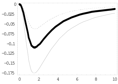
Figure 1: Plots of the Mandel parameter versus the dimensionless parameter $\frac{a}{l_{0}}$. The dotted correspond to $|\beta|^{2}=0.5$, the next correspond to $|\beta|^{2}=1$, and the uppest for $|\beta|^{2}=1.5$

This parameter vanishes for the Poisson distribution, is positive for super-Poissonian distribution (photon bunching effect), and is negative for a sub-Poissonian distribution (photon antibunchig effect).
Figure 1 shows the size dependence of the Mandel parameter for different values of dimensionless parameter$\frac{a}{l_{0}}$. As is seen, the Mandel parameter exhibit sub-Poissonian statistics and with further increasing values of $a$ it is finally stabilized at an asymptotical zero value corresponding to the Poissonian statistics.
As another important nonclassical property we examine the quadrature squeezing. For this purpose we first consider the conventional quadrature operators $\hat{X}_{a}$ and $\hat{Y}_{a}$ defined in terms of undeformed operators $\hat{a}$ and $\hat{a}^{\dagger}$ as

$$\hat{X}_{a}=\frac{1}{2}(\hat{a}e^{i\phi}+\hat{a}^{{\dagger}}e^{-i\phi})\hskip 28.45274pt\hat{Y}_{a}=\frac{1}{2i}(\hat{a}e^{i\phi}-\hat{a}^{{\dagger}}e^{-i\phi}).$$ (34)

The commutation relation for $\hat{a}$ and $\hat{a}^{{\dagger}}$ leads to the following uncertainty relation

$$(\Delta X_{a})^{2}(\Delta Y_{a})^{2}\geq\frac{1}{16}|\langle[\hat{X}_{a},\hat{Y}_{a}]\rangle|^{2}=\frac{1}{16}.$$ (35)

For the vacuum state $|0\rangle$, we have $(\Delta X_{a})^{2}=(\Delta Y_{a})^{2}=\frac{1}{4}$ and hence $(\Delta X_{a})^{2}(\Delta Y_{a})^{2}=\frac{1}{16}$. A given quantum state of the QHO is said to be squeezed when the variance of one of the quadrature components $\hat{X}_{a}$ and $\hat{Y}_{a}$ satisfies the relation

$$(\Delta O_{a})^{2}<(\Delta O_{a})^{2}_{vacuum}=\frac{1}{4}\hskip 14.22636pt(O_{a}=X_{a}\hskip 8.5359ptor\hskip 8.5359ptY_{a}).$$ (36)

The degree of quadrature squeezing can be measured by the squeezing parameter $s_{O}$ defined by

$$s_{O}=4(\Delta O_{a})^{2}-1.$$ (37)

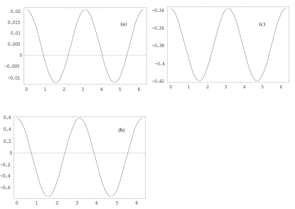
Figure 2: Plots of $s_{x_{a}}$ versus $\phi$ for $|\beta|^{2}=4$. In figure (a) we choose $a=0.5$, in figure (b) $a=1$ , and figure (c) $a=2.5$ (these value of $a$ are renormalized to $l_{0}$).

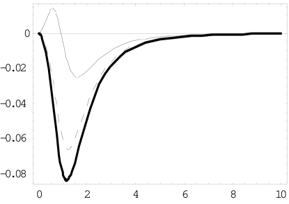
Figure 3: Plots of $s_{x_{a}}$ versus the dimensionless parameter $\frac{a}{l_{0}}$ for different phases and $|\beta|^{2}=1$. Dotted line, line and bold line ,respectively, correspond to $\phi=100$, $\phi=110$ and $\phi=90$.

Then, the condition for squeezing in the quadrature component can be simply written as $s_{O}<0$. In figure 2 we have plotted the parameter $s_{O}$ corresponding to the squeezing of $\hat{X}_{a}$ with respect to the phase angle $\phi$ for three different values of $a$. This diagram shows that the state $|\beta\rangle_{f}$ exhibit squeezing for different values of the confinement size, and maximum value of squeezing occurs when $a=1$. Figure 3 shows the plot of $s_{X_{a}}$ versus the dimensionless parameter $\frac{a}{l_{0}}$ for different values of phase. As is seen, with the increasing value of $\frac{a}{l_{0}}$ quadrature squeezing is is stabilized to zero, according to Mandel parameter.
Let us also consider the deformed quadrature operators $X_{A}$ and $Y_{A}$ defined in terms of the deformed operator $\hat{A}$ and $\hat{A}^{{\dagger}}$

$$\hat{X}_{A}=\frac{1}{2}(\hat{A}e^{i\phi}+\hat{A}^{{\dagger}}e^{-1\phi})\hskip 28.45274pt\hat{Y}_{A}=\frac{1}{2i}(\hat{A}e^{i\phi}-\hat{A}^{{\dagger}}e^{-i\phi}).$$ (38)

By considering the commutation relation for the deformed operators $\hat{A}$ and $\hat{A}^{{\dagger}}$ (6), the squeezing condition for the deformed quadrature operators $\hat{O}_{A}$ can be written as

$$S=4(\Delta O_{A})^{2}-\langle(\hat{n}+1)f^{2}(\hat{n}+1)\rangle+\langle\hat{n}f^{2}(\hat{n})\rangle<0,$$ (39)

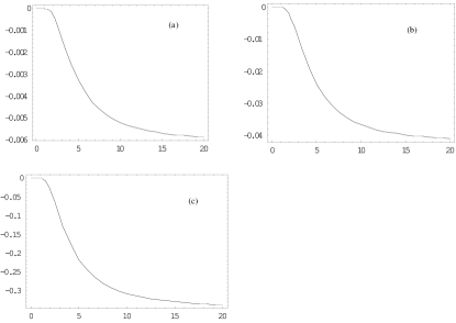
Figure 4: Plots of deformed squeezing parameter $S_{X_{A}}$ versus the dimensionless parameter $\frac{a}{l_{0}}$. Figures (a), (b) and (c), respectively correspond to $|\beta|^{2}=1$, $|\beta|^{2}=1.5$ and $|\beta|^{2}=2.5$.

where $O=X_{A}$ or $Y_{A}$. Figure 4 shows the plots of $S_{X_{A}}$ versus dimensionless parameter $\frac{a}{l_{0}}$ for three different values of $|\beta|^{2}$. As is seen, the deformed quadrature operator always exhibits squeezing.

Table 1: (Calculated energy levels of the confined QHO in a one dimensional infinite well by using our model potential in comparison with the numerical result given in Ref.[21])

state	boundary size	model potential	numerical results
0	a=0.5	4.98495312	4.95112932
0	1	1.41089325	1.29845983
0	2	0.67745392	0.53746120
0	3	0.57321464	0.50039108
0	4	0.54003728	0.50000049
1	a=0.5	19.88966157	19.77453417
1	1	5.46638033	5.07558201
1	2	2.34078691	1.76481643
1	3	1.85672176	1.50608152
1	4	1.69721813	1.50001461
2	a=0.5	44.66397441	44.45207382
2	1	11.98926850	11.25882578
2	2	4.62097017	3.39978824
2	3	3.41438455	2.54112725
2	4	3.00861155	2.50020117
3	a=0.5	79.30789166	78.99692115
3	1	20.97955777	19.89969649
3	2	7.51800371	5.58463907
3	3	5.24620303	3.66421964
3	4	4.47421754	3.50169153
4	a=0.5	123.82141330	123.41071050
4	1	32.43724814	31.00525450
4	2	11.03188752	8.36887442
4	3	7.35217718	4.95418047
4	4	6.09403610	4.50964099

4 Quantization of the EM field in confined region

4.1 Mathematical preliminary

In this section, at first we introduce a mathematical structure on Hilbert space developed recently [28]. We consider an abstract Hilbert space $\mathfrak{H}$. Let $\hat{T}$ be an operator on this space with the properties:

• $\hat{T}$ is densely defined and closed; we denote its domain by $\mathcal{D}(T)$.

• $\hat{T}^{-1}$ exists and is densely defined, with domain $\mathcal{D}(T^{-1})$.

• The vectors $\phi_{n}\in\mathcal{D}(T)\cap\mathcal{D}(T^{-1})$ for all $n$ and there exist non-empty open sets $\mathcal{D}_{T}$ and $\mathcal{D}_{T^{-1}}$ in $\mathbb{C}$ such that $\eta_{z}\in\mathcal{D}(T),\forall z\in\mathcal{D}_{T}$ and $\eta_{z}\in\mathcal{D}(T^{-1}),\forall z\in\mathcal{D}^{T^{-1}}$.

Note that the first condition implies that the operator $\hat{T}^{\ast}\hat{T}=\hat{F}$ is self-adjoint (here $\ast$ shows adjoint of operators). Due to action of the operator $\hat{T}$, the Hilbert space is transformed and orthogonal basis $\phi_{n}$ is transformed to a nonorthogonal basis. This new basis can be considered orthogonal due to a new scalar product.
We define the two new Hilbert spaces:

• $\mathfrak{H}_{F}$, which is the completion of the set $\mathcal{D}(T)$ in the scalar product

  $$\langle\psi|\phi\rangle_{F}=\langle\psi|\hat{T}^{\ast}\hat{T}\phi\rangle_{\mathfrak{H}}=\langle\psi|\hat{F}\phi\rangle_{\mathfrak{H}}.$$ (40)

  The set ${\phi_{n}^{F}=\hat{T}^{-1}\phi_{n}}$ is orthonormal in $\mathcal{H}_{F}$ and the map $\phi\rightarrow\hat{T}^{-1}\phi,\phi\in\mathcal{D}(T^{-1})$ extends to a unitary map between $\mathfrak{H}$ and $\mathfrak{H}_{F}$ . If both $\hat{T}$ and $\hat{T}^{-1}$ are bounded, $\mathfrak{H}_{F}^{-1}$ coincides with $\mathfrak{H}$ as a set.

• $\mathfrak{H}_{F}$, which is the completion of $\mathcal{D}(T^{\ast-1})$ in the scalar product

  $$\langle\psi|\phi\rangle_{F}^{-1}=\langle\psi|\hat{T}^{-1}\hat{T}^{\ast-1}\phi\rangle_{\mathfrak{H}}=\langle\psi|\hat{F}^{-1}\phi\rangle_{\mathfrak{H}}.$$ (41)

  The set ${\phi_{n}^{F^{-1}}=\hat{T}\phi_{N}}$ is orthonormal in $\mathfrak{H}_{F}^{-1}$ and the map $\phi\rightarrow\hat{T}\phi,\phi\in\mathcal{D}(T)$ extends to a unitary map between $\mathfrak{H}_{F}$ and $\mathfrak{H}_{F}^{-1}$ . If the spectrum of $\hat{F}$ is bounded away from zero then $\hat{F}^{-1}$ is bounded and one has the inclusions

  $$\mathfrak{H}_{F}\subset\mathfrak{H}\subset\mathfrak{H}_{F}^{-1}.$$ (42)

We shall refer to the spaces $\mathfrak{H}_{F}$ and $\mathfrak{H}_{F}^{-1}$ as a dual pair and when (42) is satisfied, the three spaces $\mathfrak{H}_{F}$ ,$\mathfrak{H}$ and $\mathfrak{H}_{F}^{-1}$ will be called a Gelfand triple [29].
Let $\hat{B}$ be a (densely defined) operator on $\mathfrak{H}$ and $\hat{B}^{{\dagger}}$ its adjoint on this Hilbert space. Assume that $\mathcal{D}(B)\subset\mathcal{D}(F)$. Then unless $[\hat{B},\hat{F}]=0$, the adjoint of $\hat{B}$, considered as an operator on $\mathfrak{H}_{F}$ and which we denote by $\hat{B}_{F}^{\ast}$ , is different from $\hat{B}^{{\dagger}}$. Indeed,

$$\langle\psi|\hat{B}\phi\rangle_{F} = \langle\psi|\hat{F}\hat{B}\phi\rangle_{\mathfrak{H}}=\langle\hat{B}^{{\dagger}}\hat{F}\psi|\phi\rangle_{\mathfrak{H}}=\langle\hat{F}\hat{F}^{-1}\hat{B}^{{\dagger}}\hat{F}\psi|\phi\rangle_{\mathfrak{H}}$$

$$= \langle\hat{F}^{-1}\hat{B}^{{\dagger}}\hat{F}\psi|\phi\rangle_{F}.$$

Thus

$$\hat{B}_{F}^{\ast}=\hat{F}^{-1}\hat{B}^{{\dagger}}\hat{F}.$$ (44)

Then due to the action of $\hat{T}$ on Hilbert space $\mathfrak{H}$, we obtain other space $\mathfrak{H}_{F}$. Now if we consider the oscillator operators $\hat{a}$, $\hat{a}^{{\dagger}}$ and $\hat{n}=\hat{a}^{{\dagger}}\hat{a}$, we have the following operators on $\mathfrak{H}_{F}$

$$\hat{A}_{F}=\hat{T}^{-1}\hat{a}\hat{T}\hskip 28.45274pt\hat{A}_{F}^{{\dagger}}=\hat{T}^{-1}\hat{a}^{{\dagger}}\hat{T}\hskip 28.45274pt\hat{n}_{F}=\hat{T}^{-1}\hat{n}\hat{T}.$$ (45)

Clearly, considered as operators on $\mathfrak{H}_{F}$ , $\hat{A}_{F}$ and $\hat{A}^{{\dagger}}_{F}$ are adjoints of each other and indeed they are just the unitary transforms on $\mathfrak{H}_{F}$ of the operators $\hat{a}$ and $\hat{a}^{{\dagger}}$ on $\mathfrak{H}$. On the other hand, if we take the operator $\hat{A}_{F}$ , let it act on $\mathfrak{H}$ and look for its adjoint on $\mathfrak{H}$ under this action, we obtain by (41) the operator $\hat{A}^{\sharp}=\hat{T}^{\ast}\hat{a}^{{\dagger}}\hat{T}^{\ast-1}$ which, in general, is different from $\hat{A}^{{\dagger}}_{F}$ and also $[\hat{A}_{F},\hat{A}^{\sharp}]\neq I$ , in general. In an analogous manner, we shall define the corresponding operators $\hat{a}_{F^{-1}}$, $\hat{a}^{{\dagger}}_{F^{-1}}$, etc, on $\mathfrak{H}_{F^{-1}}$. At this point we must mention, according to this mathematical structure, operators $\hat{A}_{F}$ and $\hat{A}^{\sharp}$ are exactly equivalent to generalized operators defined in (1) that were adjoint of each other on the same Hilbert space $\mathfrak{H}$.
We use this mathematical structure to find proper representation for the problem under consideration and by a constraint we will determine operator $\hat{T}$.

4.2 Quantization of fields

In previous sections, we presented a description of the quantum harmonic oscillator confined in a one dimensional infinite well and we found its associated Heisenberg-type algebra. This algebra is a deformed Heisenberg algebra which reduces to standard Heisenberg algebra when the width of the well goes to infinity.
Now using the hypothesis that successive energy levels of the QHO confined in an infinite well are obtained by creation or annihilation of quantum particles in a box, we are going to construct a quantum field theory in a confined region and using it to quantize EM field. We use canonical field quantization approach. The Lagrangian associated with a given field confined within a certain region can be written as

$$\mathpzc{L}=\mathpzc{L}_{free}+V(r).$$ (46)

where $\mathpzc{L}_{free}$ defines the Lagrangian of the free field and $V(r)=\left\{\begin{array}[]{ll}0&\textrm{$-a\leq r\leq a$}\\ \infty&\textrm{elsewhere}\end{array}\right.$. If we constrained the problem to the confined region $-a\leq r\leq a$, the $V(r)=0$ and we have $\mathpzc{L}=\mathpzc{L}_{free}$. This means that in the confined region we can use the Lagrangian of the free field. Now if we impose quantization postulate, this postulate will be the same as free space.
For example, we consider the EM field in a confined region and in this region we have the following Lagrangian for the field

$$\mathpzc{L}=-\frac{1}{4}F_{\mu\nu}F^{\mu\nu},$$ (47)

where $F_{\mu\nu}=\partial_{\mu}A_{\nu}-\partial_{\nu}A_{\mu}$ ($\mu,\nu=0,1,2,3$). As is customary in quantization of the EM field we use the four-vector potential as the dynamical variable of the field. We use the Coulomb Gauge in which $\vec{\nabla}\cdot\vec{A}=0$ and $A_{0}=0$. In this gauge, the Hamiltonian of the EM field is expressed in terms of the vector potential $\vec{A}$ as [8, 30]

$$H=\int d^{3}x\left[\left(\frac{\partial\vec{A}}{\partial t}\right)^{2}+(\vec{\nabla}\times\vec{A})^{2}\right].$$ (48)

We consider the vector potential $\hat{\vec{A}}$ as the field operator, and the quantization postulate for this field is expressed by the following commutation relation (between $\hat{\vec{A}}$ and its conjugate momentum, $\vec{E}(r)=\frac{\partial\vec{A}}{\partial t}$)

$$[\hat{A}_{i}(\vec{r},t),\hat{E}_{j}(\vec{r^{\prime}},t)]=-i\delta^{3}_{\perp ij}(r-r^{\prime}),$$ (49)

where $\delta_{\perp}$ is the transverse delta function. Now, we expand the field operator $\hat{\vec{A}}$ in terms of the ladder operators of the confined QHO (from here we show creation and annihilation operators of the confined QHO by $\hat{B}$ and $\hat{B}^{{\dagger}}$)

$$\hat{\vec{A}}=\sum_{\vec{k}}\frac{1}{\sqrt{2V\omega_{\vec{k}}}}\sum_{\lambda=1}^{2}\vec{\varepsilon}(\lambda,\vec{k})[\hat{B}_{k\lambda}u_{k}(\vec{r})+\hat{B}^{{\dagger}}_{k\lambda}u_{k}^{\ast}(\vec{r})],$$ (50)

where $\vec{\varepsilon}$ is the polarization vector of the EM field, $\lambda$ shows two independent polarization direction, and $V$ is the volume of confinement. We interpret $\hat{B}_{k\lambda}$ and $\hat{B}^{{\dagger}}_{k\lambda}$, respectively, as the annihilation and creation operators for a deformed photon (quantum excitation of the confined EM field under consideration) in direction $\vec{k}$, polarization $\lambda$ and frequency $\omega_{k}$. The electric field operator or the conjugate momentum associated with $\hat{\vec{A}}$ is given by

$$\hat{\vec{E}}(r,t)=-\frac{\partial\hat{\vec{A}}}{\partial t}=\sum_{\vec{k}}\frac{1}{\sqrt{2V\omega_{k}}}i\omega_{k}\sum_{\lambda=1}^{2}\vec{\varepsilon}(\lambda,\vec{k})[\hat{B}_{k\lambda}u_{k}(\vec{r})-\hat{B}^{{\dagger}}_{k\lambda}u_{k}^{\ast}(\vec{r})].$$ (51)

It is easy to show that

$$[\hat{\vec{A}}_{i}(\vec{r},t),\hat{\vec{E}}_{j}(\vec{r^{\prime}},t)]= \frac{-i}{2V}\sum_{\vec{k},\lambda}\varepsilon_{i}(\vec{k},\lambda)\varepsilon_{j}(\vec{k},\lambda)\times$$

$$[u_{k}(\vec{r})u_{k}^{\ast}(\vec{r^{\prime}})+u_{k}^{\ast}(\vec{r})u_{k}(\vec{r^{\prime}})]h(\hat{n}_{k,\lambda}),$$

where $[\hat{B}_{k\lambda},\hat{B}^{{\dagger}}_{k\lambda}]=h(\hat{n}_{k\lambda})=\gamma(2\hat{n}_{k\lambda}+1)+\alpha$. As is seen, in contrast to the quantization postulate (49), the right hand side of the above commutator is an operator-valued function. Hence, if we use the deformed operators $\hat{B}_{k\lambda}$, $\hat{B}^{{\dagger}}_{k\lambda}$ as amplitudes of the field expansion, the quantization postulate imposed on the canonically conjugate variables of the EM field is not preserved. To preserve the commutation relation (49), we propose using another pair of deformed operators in the Fourier decomposition of the field operator. For this purpose, we consider the following dual operator of $\hat{B}$ [31]

$$\hat{B}=\hat{a}f(\hat{n})\hskip 28.45274pt,\hskip 28.45274pt\hat{B}^{{\dagger}}_{f}=\frac{1}{f(\vec{n})}\hat{a}^{{\dagger}},$$ (53)

which satisfy the commutation relation

$$[\hat{B}_{k\lambda},\hat{B}^{{\dagger}}_{fk^{\prime}\lambda^{\prime}}]=\delta_{kk^{\prime}}\delta_{\lambda\lambda^{\prime}}.$$ (54)

We use these operators to expand the field operator

$$\hat{\vec{A}}=\sum_{\vec{k}}\frac{1}{\sqrt{2V\omega_{k}}}\sum_{\lambda=1}^{2}\vec{\varepsilon}(\lambda,\vec{k})[\hat{B}_{k\lambda}u_{k}(\vec{r})+\hat{B}^{{\dagger}}_{fk\lambda}u_{k}^{\ast}(\vec{r})].$$ (55)

As is clear, the operators $\hat{B}_{k\lambda}$ and $\hat{B}^{{\dagger}}_{fk\lambda}$ are not adjoint of each other with respect to the ordinary scalar product, so the field operator is not hermitian. It has been shown [32], there is a representation in which the operator $\hat{B}^{{\dagger}}_{f}$ is adjoint of the f-deformed operator $\hat{B}$ with respect to a new scalar product in the carrier Hilbert space. Hence, in order to preserve the quantization postulate, we should deform the Hilbert space. We show the ordinary scalar product by $\langle\,,\rangle$ and the deformed one by $\langle\,,\rangle_{f}$. Since both scalar products are defined on the same Hilbert space, they correspond to the same metric. The relation between these two scalar product according to (41) can be written as

$$\langle\phi,\psi\rangle_{f}=\langle\phi,F\psi\rangle,$$ (56)

where $F$ defines the relationship between two scalar products and it can be determined from the condition that $\hat{B}$ and $\hat{B}^{{\dagger}}_{f}$ be adjoint of each other:

$$\langle\hat{B}\phi,\psi\rangle_{f}=\langle\hat{B}\phi,F\psi\rangle=\langle\phi,\hat{B}^{{\dagger}}F\psi\rangle=\langle\phi,\hat{B}^{{\dagger}}_{f}\psi\rangle_{f}.$$ (57)

Therefore one can readily verify that $F$ is given by

$$F=f^{2}(\hat{n})\prod_{m=1}^{\infty}f^{2}(\hat{n}-m).$$ (58)

From Eqs.(41) and (58) operator $\hat{T}$ can be found as

$$\hat{T}=f(\hat{n})\prod_{m=1}^{\infty}f(\hat{n}-m).$$ (59)

and according to Eq.(45) the operators $\hat{B}_{k\lambda}$ and $\hat{B}^{{\dagger}}_{k\lambda}$ can be obtained by the action of $\hat{T}$. Now except other meaning of $T$ we can interpret it as a transformation, that by its action ordinary system can be changed to a confined system with definite barriers’s position.
Now instead of expanding the field operator in plane wave basis we expand it in a basis that is orthogonal with respect to the new scalar product (56)

$$\hat{\vec{A}}=\sum_{\vec{k}}\frac{1}{\sqrt{2V\omega_{k}}}\sum_{\lambda=1}^{2}\vec{\varepsilon}(\lambda,\vec{k})[\hat{B}_{k\lambda}v_{k}(\vec{r})+\hat{B}^{{\dagger}}_{fk\lambda}v_{k}^{\ast}(\vec{r})],$$ (60)

where $v_{k}(\vec{r})=\hat{T}u_{k}(\vec{r})$, is a basis that is orthogonal in the new representation as mentioned in mathematical preliminary section. In this new representation the field operator defined in Eq.(60) becomes Hermitian. Furthermore, the electric field operator reads as

$$\hat{\vec{E}}(r,t)=\sum_{\vec{k}}\frac{i\omega_{k}}{\sqrt{2V\omega_{k}}}\sum_{\lambda=1}^{2}\vec{\varepsilon}(\lambda,\vec{k})[\hat{B}_{k\lambda}v_{k}(\vec{r})-\hat{B}^{{\dagger}}_{fk\lambda}v_{k}^{\ast}(\vec{r})],$$ (61)

and the quantization postulate is recovered

$$[A_{i}(r,t),E_{j}(r^{\prime},t)]=-i\delta^{3}_{\perp ij}(r-r^{\prime}).$$ (62)

As mentioned before, in the confined region the Hamiltonian of the EM field is the same as in free space. This Hamiltonian in the Coulomb gauge is given by

$$\hat{H}=\frac{1}{2}\int d^{3}r\left(\hat{\vec{E}}^{2}(r)+\hat{\vec{B}}^{2}(r)\right)=\frac{1}{2}\int d^{3}r\left((\frac{\partial\hat{\vec{A}}}{\partial t})^{2}+(\vec{\nabla}\times\hat{\vec{A}})^{2}\right),$$ (63)

where $\hat{B}$ refer to the magnetic field. By substituting the field operator $\hat{\vec{A}}$ given by (60) in the above expression we arrive at the following Hamiltonian

$$\hat{H}=\sum_{k,\lambda}\omega_{k}\hat{B}^{{\dagger}}_{fk\lambda}\hat{B}_{k\lambda}.$$ (64)

Thus, the Hamiltonian can be interpreted as a collection of f-oscillators for different modes of the EM field. The eigensates of $\hat{H}$ which form a complete set and span the Hilbert space of the system, are given by

$$|0\rangle,\,\hat{B}^{{\dagger}}_{fk\lambda}|0\rangle,\,\hat{B}^{{\dagger}}_{fk\lambda}\hat{B}^{{\dagger}}_{fk^{\prime}\lambda^{\prime}}|0\rangle,\cdots,$$ (65)

where $|0\rangle$ is the vacuum state of the system i.e. $\hat{B}_{k\lambda}|0\rangle=0$. In this manner, we interpret each particle as an excitation of QHO confined in an infinite well. This formulation can be used in confined systems and nanostructures for considering elementary excitations, such as ecxitons (which is a composite excitation), phonons and plasmons.
In quantum theory of fields, there are two important concepts that are very useful in considering interacting fields. One of them is Feynman propagator which is defined for a general field operator $\hat{\psi}(x)$ as [8]

$$iD_{F}(x-y)=\langle 0|\hat{C}(\hat{\psi}(x)\hat{\psi}(y))|0\rangle,$$ (66)

where $\hat{C}$ is the time-ordered operator (we show the time ordering operator by $\hat{C}$ for making distinction between this operator and the operator $\hat{T}$ defined in (40)). Now, if we assume that the field under consideration is spatially confined, then according to the definition of the deformed scalar product given by (56) the corresponding Feynman propagator is defined as

$$iD^{\prime}_{F}(x-y)=_{f}\langle 0|\hat{C}(\hat{\psi}(x)\hat{\psi}(y))|0\rangle_{f}.$$ (67)

Making use of this definition for the photon field in a confined region and applying field operator (60) result in:

$$D^{\prime}_{F}(x-y)=F(0)D_{F}(x-y).$$ (68)

where $F(\hat{n})=f^{2}(\hat{n})\prod_{m=1}^{\infty}f^{2}({\hat{n}-m})$. Eq.(68) shows that the Feynman propagator has not any difference in confined field theory except a constant factor that depends on some physical parameters such as the size of the system, and reduces to the standard propagator when the boundaries tend to infinity. Another important concept is the scattering matrix (S matrix), that describes the probability amplitude for a process in which the system makes a transition from an initial state to a final state under the influence of an interaction. According to the concept of S matrix, the probability amplitude for a transition from the initial state $|i\rangle$ into the final state $|f\rangle$ is defined as

$$S_{fi}=\langle f|\hat{S}|i\rangle,$$ (69)

where operator $\hat{S}$ is defined in terms of the interaction Hamiltonian in the interaction picture as [8]

$$\hat{S}=\sum_{l=0}^{\infty}\frac{1}{l!}(-i)^{l}\int d^{3}r_{1}\cdots d^{3}r_{l}\hat{C}[H_{int}(t_{1})\cdots H_{int}(t_{l})].$$ (70)

In our formalism, according to the new definition of scalar product we define the probability amplitude as

$$S^{\prime}_{fi}=\langle f|\hat{S}|i\rangle_{f}=\langle f|F(\hat{n})\hat{S}|0\rangle.$$ (71)

and due to the concept of Fock states we have

$$S^{\prime}_{fi}=F(n)\langle f|\hat{S}|i\rangle=F(n)S_{fi}.$$ (72)

This equation shows that the new S matrix is proportional to the standard S matrix with a constant of proportionality that is a function of number of quantum excitations. Furthermore, we can conclude that spatial confinement of an interacting system results in an intensity-dependent coupling constant. As an example, consider an EM field that interacts with a fermionic system in a confined region. We assume that in this system, fermions be expressed by undeformed Dirac field operator denoted by $\hat{\psi}$ , and photons are described by (60). The interaction Hamiltonian can be written as

$$\hat{H}_{int}=-e\hat{\overline{\psi}}\gamma\hat{\psi}\vec{A}.$$ (73)

Therefore the $S$ matrix is given by

$$S_{fi} = 1-ieF(n)\int d^{3}x:\hat{\overline{\psi}}(x)\gamma\hat{\psi}(x)\vec{A}(x):$$ (74)

$$+ \frac{(-ie)^{2}F(n)}{2!}\int d^{3}xd^{3}y\hat{C}\left[:\hat{\overline{\psi}}(x)\gamma\hat{\psi}(x)\vec{A}(x)::\hat{\overline{\psi}}(x)\gamma\hat{\psi}(x)\vec{A}(x):\right]+\cdots$$

where the symbol $::$ denotes the normal ordering. So one can conclude from (74) that coupling constant in each term of the expansion has a same dependence on the intensity of the photon field. Dependence of coupling constant on intensity is a indication of nonlinear interaction.

5 Generation of coherent states in a confined region

In this section we consider an infinite well directed in the z-direction, in which we have a current density ($A_{0}\neq 0$). For example, an electron that moving in axial direction of the well generates the following classical current

$$\vec{j}=ev\delta(x)\delta(y)\delta(z-vt)\hat{k},$$ (75)

where $v$ is the velocity of electron. In the presence of current density, the equation of motion for the vector potential $\vec{A}$ (according to the Maxwell equations) reads as

$$\frac{1}{c^{2}}\frac{\partial^{2}\vec{A}}{\partial t^{2}}+\vec{\nabla}\times\vec{\nabla}\times\vec{A}=\frac{1}{c}\vec{j^{\prime}},$$ (76)

where $\vec{j^{\prime}}=\vec{j}-\vec{\nabla}\varphi$ is the transverse part of the current density. This equation can be derived from the Hamiltonian

$$\hat{H} = \int d^{3}r\left[\frac{1}{2}\left(\left(\frac{\partial\hat{\vec{A}}}{\partial t}\right)^{2}+\left(\vec{\nabla}\times\hat{\vec{A}}\right)^{2}\right)+\frac{1}{c}\vec{j^{\prime}}(r,t)\centerdot\hat{\vec{A}}(r,t)\right]$$ (77)

$$= \sum_{k,\lambda}\left(\omega_{k}\hat{B}^{{\dagger}}_{fk\lambda}\hat{B}_{k\lambda}\right)+\frac{1}{c}\int d^{3}r\vec{j^{\prime}}(r,t)\centerdot\hat{\vec{A}}(r,t)$$

$$= \sum_{k,\lambda}[\omega_{k}\hat{B}^{{\dagger}}_{fk\lambda}\hat{B}_{k\lambda}$$

$$+ \frac{1}{c}\frac{\vec{\varepsilon}(k,\lambda)}{\sqrt{2V\omega_{k}}}\int d^{3}r\left(\hat{B}_{k\lambda}g(k,r)+\hat{B}^{{\dagger}}_{fk\lambda}g^{\ast}(k,r)\right)\centerdot\vec{j^{\prime}}(r,t)],$$

The transverse density current $\vec{j}^{\prime}$ and the polarization vectors are in the same plane and are in the same direction. The Hamiltonian (77) can be rewritten as

$$\hat{H}=\sum_{k,\lambda}\left[\omega_{k}\hat{B}^{{\dagger}}_{fk\lambda}\hat{B}_{k\lambda}+\frac{1}{\sqrt{2V\omega_{k}}}\left(\hat{B}_{k\lambda}j^{\prime}(k,t)+\hat{B}^{{\dagger}}_{fk\lambda}j^{\prime\ast}(k,t)\right)\right].$$ (78)

where $j^{\prime}(k,t)=\frac{1}{c}\int d^{3}r\vec{\varepsilon}(k,\lambda)\cdot\vec{j}^{\prime}(r,t)g(k,r)$. The equation of motion for $\hat{B}_{k\lambda}(t)$ that follows from the above Hamitonian reads as

$$\dot{\hat{B}}=-i\omega_{k}\hat{B}_{k\lambda}-i\frac{j^{\prime\ast}(k,t)}{\sqrt{2V\omega_{k}}}.$$ (79)

If we define a new variable $\widetilde{\hat{B}}_{k\lambda}(t)=e^{i\omega_{k}t}\hat{B}_{k\lambda}$, the solution of Eq.(79) is

$$\widetilde{\hat{B}}_{k\lambda}(t)=\widetilde{\hat{B}}_{k\lambda}(-\infty)-\frac{i}{\sqrt{2V\omega_{k}}}\int_{-\infty}^{t}j^{\prime\ast}(k,t^{\prime})e^{i\omega_{k}t^{\prime}}dt^{\prime}.$$ (80)

The time dependence of the operator $\widetilde{\hat{B}}_{k\lambda}(t)$ can be regarded as a result of the following unitary transformation

$$\widetilde{\hat{B}}_{k\lambda}(t) = \hat{O}^{{\dagger}}\hat{B}_{k\lambda}(-\infty)\hat{O},$$

$$\hat{O} = \exp\left[\sum_{k,\lambda}\left(\alpha(k,t)\hat{B}^{{\dagger}}_{fk\lambda}(-\infty)-\alpha^{\ast}(k,\lambda)\hat{B}_{k\lambda}(-\infty)\right)\right].$$ (81)

where by definition $\alpha(k,t)=\frac{-i}{\sqrt{2V\omega_{k}}}\int_{-\infty}^{t}j^{\prime\ast}(k,t^{\prime})e^{i\omega_{k}t^{\prime}}dt^{\prime}$. The operator $\hat{O}$ is a displacement-like operator [31, 32]. If we choose the initial state of the EM field to be the vacuum $|0\rangle$, then the state vector at time $t$ is

$$|\beta(k,t)\rangle = \hat{O}|0\rangle=\exp\left[\sum_{k,\lambda}\left(\beta(k,t)\hat{B}^{{\dagger}}_{fk\lambda}(-\infty)-\beta^{\ast}(k,\lambda)\hat{B}_{k\lambda}(-\infty)\right)\right]|0\rangle$$ (82)

$$= e^{-\frac{|\beta(k,t)|^{2}}{2}}\sum_{n}\frac{\beta^{n}(k,t)}{[f(n)]!n!}(\hat{a}^{{\dagger}})^{n}|0\rangle$$

$$= e^{-\frac{|\beta(k,t)|^{2}}{2}}\sum_{n}\frac{\beta^{n}(k,t)}{\sqrt{n!}[f(n)]!}|n\rangle.$$

In the sense of Eqs.(11)-(13) it is evident that this state can be regarded as a nonlinear coherent state.

6 Conclusion

In this paper, we have considered the relation between the spatial confinement effects and special kind of f-deformed algebra. We have found that the confined simple harmonic oscillator can be interpreted as an f-oscillator, and we have obtained the corresponding deformation function. Then we have searched the effects of boundary conditions in quantum field theory. We have used f-deformed operators as the dynamical variables and found that for preserving commutation relation between the field operator and its conjugate momentum we should deform Hilbert space of the system under consideration. As a result of new definition of scalar product, we have concluded that the coupling constant of interactions in confined systems become a function of number of excitation, for example in the case of EM field coupling constant becomes a function of intensity of EM field. Finally we have proposed a theoretical scheme for generating nonlinear coherent states of EM field through the coupling of a classical current to the vector potential operator $\hat{\vec{A}}$ inside a confined region.

References

References

-
[1]
D. K. Ferry, S. M. Goodnick, Transport in
nanostructures, (Cambridge University Press 1999).
B. L. Altshuler, P. A. Lee, R. A. Web, Mesoscopic phenomena in solids, (North-Holland, Amsterdam 1991). - [2] G. Plunien, B. Müller, W. Greiner, Phys. Rep. 134, 87 (1986).
- [3] H. Haug, S. W. Koch, Quantum theory of the optical and electronic properties of semiconductors, 4th ed. (World Scientific, Singapore, 2004).
- [4] P. Michler, Single quantum dots: Fundamental, Application, and new concepts, Topics in applied physics (Springer, 2003).
-
[5]
P. Michler, A. Imamoğlu, M. D. Mason, P. J.
Carson, G. F. Strouse, S. K. Buratto, Nature
(London)406, 968 (2000);
P. Michler, A. Kiraz, C. Becher, W. V. Shoenfeld, P. M. Petroff, L. Zhang, E. Hu, A. Imamoğlu, Science 290, 2282 (2000). - [6] P. Michler, A. Kiraz, L. Zhang, C. Becher, E. Hu, A. Imamoğlu, Appl. Phys. Lett. 77, 184 (2000).
-
[7]
T. Feldtmann, L. Schneebeli, M. Kira, S. W. Koch, Phys.
Rev. B 73, 155319 (2006);
C. Gies, J. Wiersing, M. Lorke, F. Jahnke, Phys. Rev A 75, 013803 (2007);
K. Ahn, J. Förstner, A. Knorr, Phys. Rev. B 71, 153309 (2005). -
[8]
W. Greiner, J. Reihardt, Field
quantization (Springer-Verlag 1996).
Steven Weinberg, The quantum theory of fields Vol.1 (Cambridge University Press 1995). - [9] V. I. Man’ko, G. Marmo, G. C. E. Sudarshan, F. Zaccaria, Phys. Scr. 55, 528 (1997).
-
[10]
V. I. Man’ko, R. Vilela Mendes, J. Phys. A: Math.
Gen.
31, 6037 (1998);
V. I. Man’ko, G. Marmo, S. Solimeno, F. Zaccaria, Int. J. Mod. Phys. A 8, 3577 (1993);
V. I. Man’ko, G. Marmo, S. Solimeno, F. Zaccaria, Phys. Lett. A 176, 173 (1993). - [11] V. I. Man’ko, G. Marmo, E. C. G. Sudarshan, and F. Zaccaria, in: N. M. Atakishiev (Ed), Proc. IV Wigner Symp. (Guadalajara, Mexico, July 1995), World Scientific, Singapore, 1996, P.421; S. Mancini, Phys. Lett. A 233, 291, 55 (1997); S. Sivakumar, J. Phys. A: Math. Gen. 33, 2289 (2000); B. Roy, Phys. Lett. A 249, 55 (1998); H. C. Fu, R. Sasaki, J. Phys. A: Math. Gen. 29, 5637 (1996); R. Roknizadeh, M. K. Tavassoly, J. Phys. A: Math. Gen. 37, 5649 (2004); M. H. Naderi, M. Soltanolkotabi, R. Roknizadeh, J. Phys. A: Math. Gen. 37, 3225 (2004); A-S. F. obada, G. M. Abd Al-Kader, J. Opt. B: Quantum Semiclass. Opt. 7, S635 (2005).
- [12] R. L. deMatos Filho, W. Vogel, Phys. Rev. A 54, 4560 (1996).
- [13] M. H. Naderi, M. Soltanolkotabi, R. Roknizadeh, Eur. Phys. J. D 32, 397 (2005).
- [14] M. H. Naderi, PhD Thesis, University of Isfahan, Iran (unpublished 2004).
- [15] A. Mahdifar, R. Roknizadeh, M. H. Naderi, J. Phys. A: Math. Gen. 39, 7003 (2006).
- [16] V. B. Bezzera, M. A. Rego-Monteiro, Phys. Rev. D 70, 065018 (2004).
- [17] E. M. F. Curado, M. A. Rego-Monteiro, J. Phys. A: Math. Gen. 34, 3253 (2001).
- [18] P. Narayana Swamy, Physica A 353, 119 (2005).
- [19] M. H. Naderi, M. Soltanolkotabi, R. Roknizadeh, J. Phys. Soc. Japan 73, 2413 (2004).
- [20] S. Sivakumar, Phys, Lett. A 250, 257 (1998); V. I. Man’ko, A. Wünshe, Quantum Semiclass. Opt. 9, 381 (1997); G. N. Jones, J. Haight, C. T. Lee, Quantum Semiclass. Opt. 9, 411 (1997); V. V. Dodonov, Y. A. Korennoy, V. I. Man’ko, Y. A. moukhin, Quantum Semiclass. Opt. 8, 413 (1996); Nai-li Liu, Zhi-hu Sun, Hong-yi Fan, J. phys. A: Math. Gen. 33, 1993 (2000);B. Roy, P. Roy, J. Opt. B: Quantum Semiclass. Opt. 1, 341 (1999).
-
[21]
G. Campoy, N. Aquino, V. D. Granados, J. Phys. A:
Math. Gen.
35, 4903 (2002);
- [22] V. C. Aguilera-Navarros, E. Ley Koo, A. H. Zimerman, J. Phys. A: Math. Gen. 13, 3585 (1980).
- [23] C. Zicovich-Wilson, J. H. Planelles, W. Jackolski, Int. J. Quan. Chem. 50, 429 (1994).
- [24] L. Infeld, T. E. Hull, Rev. Mod. Phys. 23, 21 (1951).
-
[25]
J. R. Klauder, B. Skagerstam, Coherent states: Application in Physics and Mathematical
Physics (World Scientific, Singapore, 1985).
S. T. Ali, J-P. Antoine, J-P. Gazeau, Coherent states, Wavalets, and their generalization (New York: Springer 2000) - [26] G. N. Watson, Theory of Bessel functions, Second ed. (Cambridge University Press 1966) P.388.
- [27] L. Mandel, E. Wolf, Optical coherence and quantum optics (Cambridge University Press 1995).
- [28] S. Twareque Ali, R. Roknizadeh, M. K. Tavassoly, J. Phys. A: Math. Gen. 37, 4407 (2004).
- [29] M. I. Gelfand, N. Ya Vilenkin, Generalized functions Vol. 4 (New York: Academic Press 1964).
- [30] W. Hitler, The quantum theory of radiation, Third Edition (Clarendo Press 1954).
-
[31]
B. Roy, Phys. Lett. A 249, 25 (1998);
B. Roy, P. Roy, Phys. Lett. A 263, 48 (1999). - [32] P. Aniello, V. Man’ko, G. Marmo, S. Solimeno, F. Zaccaria, J. Opt. B: Quantum Semiclass. Opt. 2, 718 (2000).