A Statistical Description of Parametric Instabilities with an Incoherent Pump

Abstract

The effect on parametric instability growth of pump wave incoherence is treated by deriving a set of equations governing the space-time evolution of the ensemble-average coupled-mode amplitudes and intensities. Particular attention is paid to establishing the regions of validity of the statistical description. Thresholds, growth rates, and amplification rates are given for both spatially and temporally incoherent pump waves. Both absolutely and convectively unstable modes are considered. The statistical results are verified where appropriate by numerical integration of the coupled-mode equations with different models of pump incoherence.

I Introduction

The requirements of laser fusion targets for high power lasers with good laser beam uniformity has driven a quest for new techniques for smoothing the intensity variations on the target surface. Early attempts at beam smoothing[1] were not well characterized but more systematic techniques[2-6] have demonstrated significant improvements in beam uniformity. All techniques involve introduction of phase nonuniformities which replace the normal beam pattern, typically containing substantial hotspots, with a smaller-length-scale speckle pattern. Further addition of bandwidth to the laser provides temporal smoothing of the speckle. The primary motivation for investing in these smoothing schemes is to reduce the initial nonuniformities that can seed fluid instabilities such as Rayleigh-Taylor, yet there is also palpable interest in reducing the strength of laser plasma instabilities such as stimulated Raman or Brillouin scattering or two plasmon decay. Supplying a theoretical framework for understanding these laser plasma interactions with smoothed laser beams is the task we undertake in this article. In a subsequent article[7], the results obtained here will be applied to particular instabilities in geometries of interest.

With the usual assumptions about slow variation of parameters with respect to the frequencies $\omega_{j}$ and wave vectors k_j of the wave, the coherent and incoherent problems can be studied within the context of the coupled mode equations (II.10 or II.7). The wave group velocities and damping rates are denoted by V_j and $\nu_{j}$ respectively; the strength of the coupling between the waves, $\gamma_{0}$, proportional to the pump or laser wave amplitude, has the dimensions of frequency and is the rate at which the waves grow without damping in an infinite homogeneous plasma. As the reader will remember, for a coherent driver, both convective and absolute instability may occur provided the laser intensity, i.e. $\gamma_{0}^{2}$, exceeds certain threshold values set by losses [8]. In an unbounded plasma, the convective coherent threshold is

$$\gamma_{0}^{2}=\nu_{1}\nu_{2}.$$

Absolute instability requires that the decay waves be oppositely directed $(V_{1}V_{2}<0)$, and, the absolute coherent threshold is

$$\gamma_{0}=\sqrt{\mid V_{1}V_{2}\mid\over 2}({\nu_{1}\over\mid V_{1}\mid}+{\nu_{2}\over\mid V_{2}\mid})$$

Temporal and spatial incoherence introduce two additional parameters, the temporal bandwidth $\Delta\omega_{0}$ and the spatial bandwidth (or spread in wavevectors) $\Delta k_{0}$ which is inversely related to the correlation length $X_{c}$.

The effects of both temporal and stationary spatial pump incoherence on parametric instabilities in homogeneous and inhomogeneous plasma has been studied extensively both theoretically and experimentally over the past thirty years [9-68]. The first approach was quite naturally to consider the purely temporal problem with coupled mode equations in homogeneous plasma. Zaslavskii and Zakharov [9] considered the generic undamped decay instability with methods developed earlier for studying the relaxation of two level molecular systems driven by an external field [10]. They found that the convective growth rate was reduced, in the limit $\gamma_{0}\ll\Delta\omega$, from $\gamma_{0}$ to $\gamma_{0}^{2}/\Delta\omega$. Both Valeo and Oberman [11] and Tamor [12] addressed this problem with different methods and obtained the same result. Tamor included a damping rate on the Langmuir wave coupled to an acoustic wave and found a dispersion relation where the damping rate for the Langmuir wave $nu_{p}$ is replaced by $\nu_{p}+2\Delta\omega$. He noted reasonably that the bandwidth was unimportant unless it exceeded the damping rate $\nu_{p}$ but made no comment on the fact that the bandwidth appeared asymmetrically in his dispersion relation; that is, the apparent damping of the acoustic wave was unaffected. In a series of articles [13-15], Thomson made a number of important contributions. First, he noted that for equal damping on both modes, the threshold was $\gamma_{0}^{2}=\nu\Delta\omega$ if $\Delta\omega\gg\nu$ and incorrectly speculated that, for unequal damping, the threshold was $\gamma_{0}^{2}=\Delta\omega\nu_{1}\nu_{2}/{\rm min}(\nu_{1},\nu_{2})$. This guess was based on the assumption that, for growth to occur in either mode, the average amplitude of both must grow.

The correct solution was presented by Thomson[15] later using an exactly solvable model [69]. For the purely temporal problem, the ensemble-averaged mode amplitude equations showed these equations decouple and have ${\it different}$ thresholds, i.e.

$$\gamma_{0}^{2}=\Delta\omega_{0}\nu_{1},$$

and

$$\gamma_{0}^{2}=\Delta\omega_{0}\nu_{2}$$

Thomson noticed and explained the asymmetry as due to averaging over the rapidly varying phase of the mode amplitude. He obtained a more appropriate threshold by solving the equations for the ensemble averaged intensities. The solution showed that the lower of the thresholds (I-3,4) was appropriate. We show, as did Thomson, that the incoherent growth rate for the average intensity is

$$\gamma_{inc}=2\gamma_{0}^{2}/\Delta\omega_{0}$$

provided $\nu_{1}<\gamma_{inc}<\nu_{2}$. This answer is expected, given that the average amplitudes grow with rate $\gamma_{0}^{2}/\Delta\omega_{0}$. However, Thomson did not point out the interesting fact (found also by Laval et al.[16] in the space-time problem when $|V_{1}|=|V_{2}|$) that, if $\gamma_{inc}>\nu_{1},\nu_{2}$, the incoherent growth rate is

$$\gamma_{inc}=4\gamma_{0}^{2}/\Delta\omega_{0},$$

that is twice the expected rate. We will comment more on this in Secs. V-VII. Thomson then considered the space time problem with the ensemble averaged mode amplitude equations and again found an asymmetry in the thresholds for the absolute instability when $\Delta\omega_{0}>>\nu_{j}$. Thomson naturally assumed that the appropriate intensity threshold, in analogy with the temporal problem, was the lower one. Later work showed this to be incorrect.

Laval et al. reconsidered [70] the space -time problem for the evolution of the intensities both by using the Bourret approximation and, in the case $V_{0}=\infty$, the exactly solvable Kubo-Anderson process (KAP). They showed that the intensity thresholds are in fact much lower than the amplitude thresholds when $\Delta\omega_{0}>>\nu_{j}$ and, in usual cases of interest ($\nu_{2}>V_{2}\nu_{1}/V_{1}$), the incoherent absolute threshold equals the product of the bandwidth and the damping on the slow wave

$$\gamma_{0}^{2}=\Delta\omega_{0}\nu_{2}.$$

In a later publication [17], Thomson applied the results to stimulated Raman forward scatter and incorrectly concluded, as we discuss subsequently, that small amounts of bandwidth, comparable to its growth rate, can suppress this slowly-growing instability. During this time period, the nonlinear evolution of instabilities driven by broadband pumps was investigated by using particle-in-cell (PIC) simulations [18-20]. These studies demonstrated a reduction in the stimulated Brillouin reflectivity from 60% to less than 10% with 5% bandwidth. Because these plasmas were strongly inhomogeneous, no reduction is expected for modest bandwidth, $\Delta\omega\simeq\gamma_{0}$, as shown by Thomson [15]. However, with $\Delta\omega/\omega_{0}\simeq.05$, the line separations in these simulations are larger than an acoustic frequency and each line acts independently. Kruer et al. [19] also suggest that bandwidth in an inhomogeneous plasma will be ineffective unless $\Delta\omega\geq V_{0}/l$ where $l$ is the interaction length set by plasma inhomogeneity. This can be rephrased in terms of the correlation length, $x_{c}=V_{0}/\Delta\omega<=l$ where $l=\gamma_{0}/\kappa^{\prime}(|v_{1}v_{2}|)^{1/2}$ and $\kappa^{\prime}=dk_{\Delta}(x)/dx$ for $k_{\Delta}=k_{0}-k_{1}-k_{2}$; $k_{\Delta}=0$ is the condition for phase matching. Kruer’s condition is difficult to satisfy for typical laser systems. We return to this subject in our discussion of spatial incoherence effects. The correct theory [15] for convective amplification in an inhomogeneous plasma showed that the growth rate was reduced but the ensemble-averaged mode amplitude convectively saturates at the same level as the coherently driven amplitude. (Thomson actually misstated his result, although his analysis was correct. Later work [45,49] that solved the coupled mode equations clarified the answer.)

Estabrook et al. also considered, with PIC simulations, the effect of laser bandwidth on stimulated Raman scattering– again in inhomogeneous plasma. Bandwidth was represented by a series of equally spaced laser lines. A reduction in the reflectivity was found when the line separation was greater the growth rate. Each line acted as an independent pump, and the intensity was low enough that the instability was not strongly saturated. Direct comparisons between homogeneous plasma theory and PIC simulations of SRS in a plasma slab were made by Forslund et al. [21] with good agreement for the dependence of the SRS growth rate on the bandwidth of the frequency modulated laser. These authors pointed out that, $\Delta\omega/\gamma_{0}\geq 2$, despite a fourfold reduction in the growth rate, only a modest reduction in the power reflected was observed in the final state. A further increase of bandwidth to $\Delta\omega/\gamma_{0}\geq 10$ brought the instability below threshold. Later PIC work [24] with multiple lines also showed good agreement with theory for the Raman backscatter growth rate when $\gamma_{0}/\Delta\omega\ll 1$ at several combinations of density and laser intensity. These simulations also showed a monotonic decrease with bandwidth in the absorption into hot electrons due to SRS and in the SRS reflected power. Less effect on the forward SRS was observed, consistent with the theory we discuss subsequently. Other theoretical work on pump bandwidth effects concerned applications to specific targets [30], and the application to induced spatial incoherence (ISI) [44]. The effects of both temporal and spatial bandwidth in a 1D inhomogeneous plasma [45] for a phase mismatch, $k_{0}(x)-k_{1}(x)-k_{2}(x)=k_{\Delta}(x)$, varying linearly, $k_{\Delta}(x)=\kappa^{\prime}x$, or quadratically, $k_{\Delta}(x)=\kappa^{\prime\prime}x^{2}/2$, was treated by analytical and numerical methods. In reference [47], the Green’s function formalism of Brissaud and Fritsch [69], used by other authors [15,16,38] was reformulated in the language of effective Hamiltonian matrices. In a second paper[48], this formalism was used to investigate the competition between temporal bandwidth and inhomogeneity for a variety of parametric processes, including two plasmon decay. Early experiments [25,26] that attempted to observe laser bandwidth effects utilized plasmas that were too nonuniform to expect observable effects. Later experiments used gas jet targets [27,29] or used microwave plasmas [28]. Clayton et al. and Giles et al. divided the laser power into two lines and found a striking reductions in reflected SBS power compared to a single line with the same total laser power. The lines were separated by much more than a growth rate.

It was recognized early [31-33] that random spatial modulation of the phase mismatch, $\phi=\int dxk_{\Delta}(x)$, could also reduce parametric instability growth rates. Using methods similar to the temporal problem, Kaw et al. used the steady-state limit of the coupled-mode equations (II-10) to find a convective gain rate, $\gamma_{0}^{2}/4\Delta|v_{1}v_{2}|$, where $\Delta=<\delta k^{2}>l_{c}$. Here $\delta k$ is the wavevector mismatch induced by the random variation in the plasma properties and $l_{c}$ is the correlation length for the random process. Further work [34-38,40-42] on random fluctuations of the phase concerned its effect on the growth in inhomogeneous plasmas where, for example, the stabilization of absolute modes by linear gradients in the phase could be undone by these fluctuations. In this article, we concentrate on the effects in uniform plasmas.

Beam smoothing techniques use not only temporally incoherent but also spatially incoherent pump waves. In the focal plane, the laser wave can be considered a sum of randomly phased plane waves with a spread in wavevectors, $\Delta k_{0}$. In the limit of no temporal bandwidth, the spatial interference pattern of the pump wave envelope is stationary and is related to the effect of stationary plasma turbulence on parametric instability treated by Williams et al.[39] Using a novel approach (unrelated to the methods used in the present analysis), they considered the threshold and growth rate for absolute modes in a finite system of length L. This analysis finds that for sufficiently large spatial bandwidth, $\Delta k_{0}$, the fastest growth rate is reduced from the coherent absolute rate,

$$\gamma=\gamma_{0}{\sqrt{\mid V_{2}V_{1}\mid}\gamma_{0}\over\mid V_{1}\mid+\mid V_{2}\mid}$$

when $\nu_{j}=0$ to the spatially incoherent absolute rate

$$\gamma=\gamma_{0}^{2}{\rm ln}(\mid\Delta k_{0}\mid L)/\mid\Delta k_{0}\mid(\mid V_{1}\mid+\mid V_{2}\mid),$$

(To obtain I-9 from Eq. 52 of Williams et al., the reader is advised that the correct normalization for the growth rate is $\gamma_{0}\sqrt{\mid V_{1}V_{2}\mid}/(\mid V_{1}\mid+\mid V_{2}\mid).$ Their Eq. 3 is incorrect.) The incoherent result in Eq. (I-9) must of course be less than the coherent one in Eq. (I-8). The unexpected feature of (I-9) is the length dependent logarithmic factor which is related to the fact that the rate (I-9) is not the average rate sought in our analysis but the largest rate expected in a system of length L. Except for the logarithmic factor, we recover the scaling of the result of Eq. (I-9). In the present article, we derive average amplitude equations by using the Bourret approximation[70] and average intensity equations by using the so- called random phase approximation (RPA).[71-74] The major objective of this article is to provide a unified theory of spatial and temporal incoherence effects on parametric instabilities. The approximations and assumptions necessary to arrive at the RPA equations (V.32) and the Bourret equations (V.1 4) that form the basis for theoretical results in Sec. VI are carefully explored and systematically presented in Sec. III through V. A comprehensive set of results is presented for the threshold and growth rate of both absolute and convective instability in the incoherent limit. The domains of validity of the statistical approximations are explicitly noted and outside these domains the coherent results are shown to apply. Moreover the same analysis is done for the spatial amplification of convectively unstable waves. Finally, we present in Sec. VII numerical solutions of the fundamental set of equations (II-10) for particular models of incoherence that illustrate the meaning of the averaging procedures and verify the main results.

The RPA dispersion relation (VI.1) for an infinite system obtained from the RPA equations (V.32) form the basis for the analysis of growth rates and thresholds in Section VI. There are two parameters that play a role in the ensemble average equations that measure the effective bandwidth, $\Delta\omega_{j},j=1,2$ where

$$\Delta\omega_{j}\equiv\Delta\omega_{0}\mid(1-V_{jx}/V_{0})\mid+\mid\Delta k_{0}\cdot V_{j}\mid$$

In the general case of spatial and temporal incoherence, there can be a gap between the domain of validity for the RPA dispersion relation and the coherent one. The coherent domain is the whole region where either spectral width $\Delta\omega_{j}$ is less than the corresponding damping rate or growth rate.In this intermediate region, the average amplitude dispersion relations (VI.2) are valid, and the more unstable one agrees with the RPA dispersion relation within a factor of two. It is on this basis that we argue that the RPA dispersion relation can be used in the whole domain (denoted the incoherent domain) complementary to the coherent domain.

In the remainder of Sec. VI, a description of parametric instabilities is given including the conditions for absolute and convective instability. Both early time behavior, which is dominated by convective instability, and long time behavior, which is dominated by absolute instability (if it exists) or by spatial amplification are considered. It is worth noting that, in the incoherent domain, the average amplitude dispersion relations (VI.2) allow only convective solutions whereas the RPA dispersion relation (VI.1) allows the possibility of absolute instability if a threshold can be exceeded. However, the simpler average amplitude equations do provide the convective mode threshold (VI.5), growth rate (VI.7), and spatial amplification factor (VI.13) and (VI.16) (within better than a factor of two) in agreement with those obtained in Sec. VI using the RPA dispersion relation.

Absolute instabilities are of particular practical interest because, above threshold, the only limit to their growth is the finite laser energy or other nonlinear effects. On the other hand, an absolute instability generally has a larger threshold to overcome losses to collisional or Landau damping than a convective instability. For a coherent laser wave, the threshold laser intensity is determined by setting the spatial growth rate $\gamma_{0}/\mid V_{1}V_{2}\mid^{1/2}$ equal to one-half of the sum of the spatial loss rates $\nu_{j}/\mid V_{j}\mid$ for the decay modes (Eq. I-2). In addition, as given by Eq. (I-8), the absolute instability growth rate is smaller than the growth rate $\gamma_{0}$ by approximately the ratio $(\mid V_{2}/V_{1}\mid)^{1/2}$ in the usual case $\mid V_{2}/V_{1}\mid<<1$. The exact formula is also given by Eq. (VI.11). With incoherent laser beams, the threshold is still determined by setting the effective spatial growth rate equal to the sum of loss rates but now the spatial growth rate is ${\rm Max}(\gamma_{0}^{2}/2\Delta\omega_{j}\mid V_{j}\mid)$, that is, the maximum spatial growth rate for the average amplitude equations. The general formula is given by (VI.9). Note in the special but interesting case that $\Delta\omega_{1}=\Delta\omega_{2}=\Delta\omega_{0}$, temporal incoherence

increases the absolute threshold if $R_{a}=(\gamma_{0}/\Delta\omega_{0})(\sqrt{\mid V_{1}V_{2}\mid}/{\rm Min}\mid V_{j}\mid)<1$ which exceeds the naive criterion by the square root of the group velocity ratio. We observe that the statement $R_{a}<1$ is equivalent to requiring that the coherent spatial growth length $\mid V_{1}V_{2}\mid^{1/2}/\gamma_{0}$ exceed the larger coherence length $\mid V_{1}/\Delta\omega_{1}\mid$. A rigorous application[46] of the Bers and Briggs criteria[75] arrives at this same condition as a necessary condition (VI.10) for the incoherent limit to apply. Above the incoherent threshold, the incoherent absolute growth rate is roughly $\gamma_{0}^{2}/\Delta\omega_{1}$, (the exact formula is given by Eq. (VI.8)) i.e. approximately the same expression as the incoherent convective growth rate but with a different domain of validity.

There is a limit where the effective bandwidths $\Delta\omega_{j}$ are determined only by spatial incoherence. Then $\mid\Delta\omega_{j}/V_{j}\mid=\Delta k_{0}$ is independent of the group velocity and the growth rate,

$$\gamma^{abs}_{\langle a^{2}\rangle}=4\gamma_{0}^{2}/\mid\Delta k_{0}\mid(\mid V_{1}\mid+\mid V_{2}\mid),$$

agrees with the scaling found previously and given in Eq. (I-9). Thus our general threshold and growth rate formulae indeed recover the correct limits of purely spatial and purely temporal incoherence derived previously. The coherent convective threshold, always lower than that for absolute instability, is given by the requirement that the growth rate $\gamma_{0}$ be greater than the mean loss rate $(\nu_{1}\nu_{2})^{1/2}$. The same criterion for an incoherent pump applies if the laser intensity is reduced by the ratio of line widths factor $R_{c}\equiv\nu_{1}/\Delta\omega_{1}+\nu_{2}/\Delta\omega_{2}$. The effective bandwidth $\Delta\omega_{j}$ must be larger than the corresponding damping rate $\nu_{j}$ for each mode to increase the threshold. Otherwise the coherent threshold applies (I-1). Far above the incoherent threshold, the incoherent convective growth rate is reduced by the factor $\gamma_{0}/{\rm Min}(\Delta\omega_{j})$. Note that when $\Delta\omega_{j}\simeq\Delta\omega_{0}$ the convective and absolute incoherent growth rates are equal in the overlapping domain of validity. More exact expressions are given by (VI.5) - (VI.7).

For many cases of practical interest $\Delta\omega_{j}\sim\Delta\omega_{0}$ because the spread in laser wavenumbers is sufficiently small and/or the group velocity is small enough that $\mid\Delta k_{0}\cdot V_{j}\mid<<\Delta\omega_{0}$ and either $\mid V_{j}/V_{0}\mid<<1$ or $V_{j}/V_{0}<0$. Then temporal incoherence is the dominant stabilizing influence. However two special cases deserve mention. Examination of the expression (VI.8b) for the absolute instability growth rate above threshold shows that if the maximum value of the coherence length $V_{j}/\Delta\omega_{j}$ occurs for the minimum group velocity, the growth rate is strongly reduced $\gamma^{abs}=V_{2}\gamma_{0}^{2}/V_{1}\Delta\omega_{2}$ in the usual case $\mid V_{2}\mid<<\mid V_{1}\mid$. This case can occur if there is a large spread in wavenumber accompanied by a weak temporal incoherence so that $\gamma^{abs}=\gamma_{0}^{2}/\mid\Delta k_{0}\cdot V_{1}\mid$. The transient or convective growth rate for the same case (in the incoherent limit) is larger, $\gamma conv=\gamma_{0}^{2}/\mid\Delta k_{0}\cdot V_{2}\mid$. The other unusual case occurs in the case of temporal incoherence for forward scatter when $V_{1}\sim V_{0}$. Then $\Delta\omega_{1}=\Delta\omega_{0}(1-V_{1}/V_{0})<<\Delta\omega_{0}$ so that the coherent convective growth still occurs even if $\Delta\omega_{0}\sim\gamma_{0}$. The case of practical interest is stimulated Raman forward scatter.[22-24]

The fate of absolutely unstable modes necessarily requires consideration of nonlinear effects but, in a bounded plasma, the maximum amplitude of convectively unstable waves may be found by computing the spatial amplification rate. In general there are two roots that are most easily obtained by using the average amplitude equations (VI.2) but are also accessible from the average intensity equations (VI.1). A bandwidth $\Delta\omega_{0}>\gamma_{0},\nu_{j}$ is usually sufficient to reduce the spatial growth rate. For moderate intensities, i.e., below any absolute threshold, the spatial gain coefficient $\kappa\sim\gamma_{0}^{2}/\Delta\omega_{0}V_{1}$ (where $\mid V_{1}\mid>\mid V_{2}\mid$) is reduced by $(\gamma_{0}/\Delta\omega_{0})(V_{2}/V_{1})^{1/2}$ in the weak damping case. At higher intensities, a second root with gain coefficient $\kappa\sim\gamma_{0}^{2}/\Delta\omega_{0}V_{2}$ occurs provided $\Delta\omega_{0}>\gamma_{0}(\mid V_{1}/V_{2})^{1/2}$ and $\gamma_{0}^{2}>\Delta\omega_{0}\nu_{2}$, that is, above the absolute mode threshold when $V_{1}V_{2}<0$. Therefore both a convective and absolute mode exist; and, interestingly, the convective mode has a spatial gain rate that exceeds that of the absolute mode. A more detailed discussion and exact formulae are given in Eqs. (VI.12) - (VI.18).

In the general case, it is difficult to summarize the effects of incoherence on convective and absolute stabilities. However, it is useful to consider a common case of practical interest where $\mid V_{1}/V_{2}\mid>>1$ and $\Delta\omega_{1}\simeq\Delta\omega_{2}\equiv\Delta\omega_{0}$. Then diagrams showing stability regions can be constructed with axes $\Delta\omega_{0}/\gamma_{0}$ and $\nu_{2}/\nu_{0}$, i.e. moving towards more incoherence in one direction and towards more damping in the other. Figure VI.1 is such a diagram for convectively unstable modes. There are four regions: coherently unstable, incoherently unstable with reduced growth rate, coherently stable, and incoherently stabilized. In Fig. VI.2, the diagram for absolutely unstable modes is drawn with four analogous regions. This figure graphically shows that, in only a small region of parameter space does incoherence reduce the growth rate but not completely stabilize. Figure VI.3 shows the different regions for spatial amplification. Finally, in Fig. VI.4, an overall diagram is shown for all regions for convective, absolute, and spatial amplification.

To this point, we have presented results for infinite homogeneous plasma. For a large enough system, these results are a good guide to the behavior in finite systems. Nonetheless, real plasmas are finite and it is well known that a threshold length is necessary for absolute instability. Moreover in Sec. VII, numerical solutions of the coupled mode equations (II.10) are presented in a necessarily finite system. Thus partly as a guide to the numerical solutions, we find the threshold length for absolute instability in the coherent and incoherent limit as obtained by solving Eq. (II-10) or Eq. (V.32) as appropriate. It is an interesting feature that the normal modes in the slab, sinusoidal in the coherent limit, are exponential in the incoherent limit. The threshold length given by Eq. (VI.30) increases as expected with bandwidth above the coherent threshold length (VI.29).

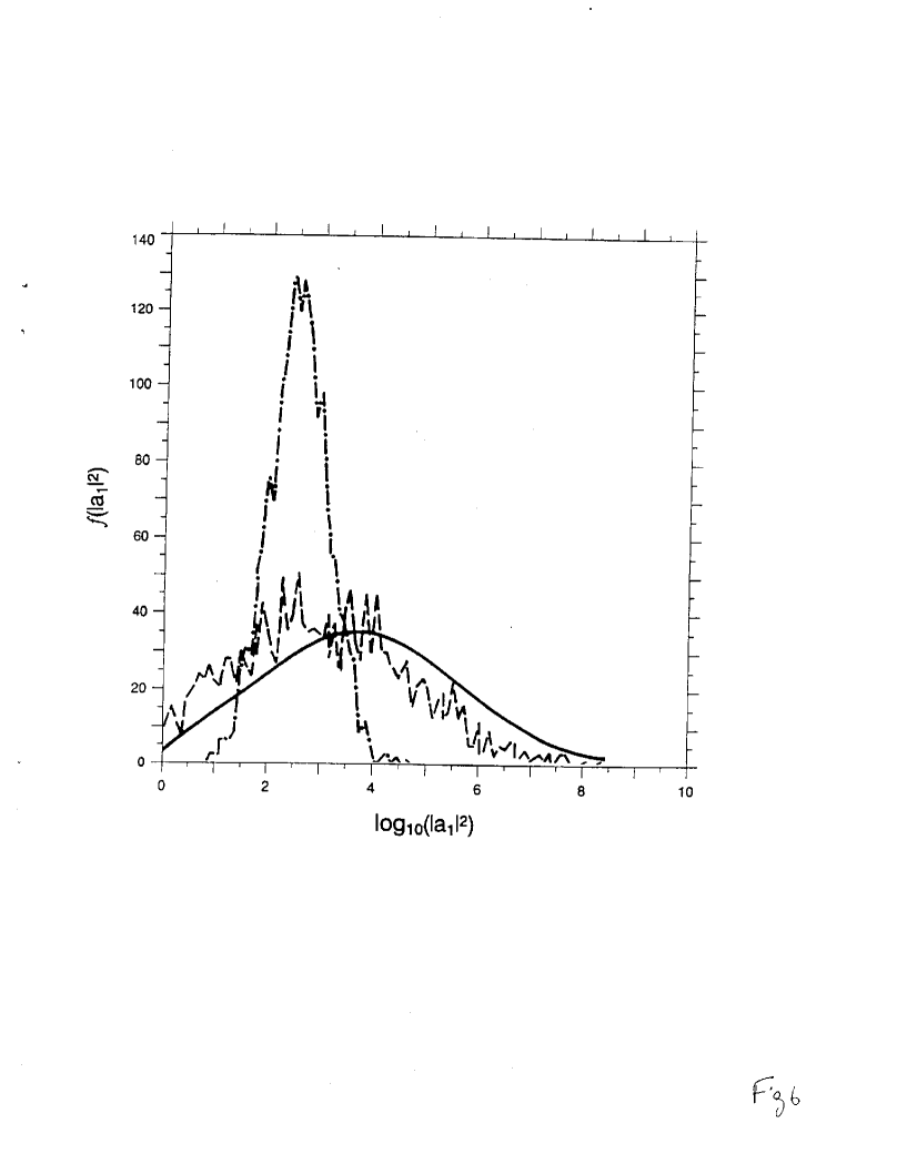
Figure 6: Distribution of the intensity $\mid a_{1}\mid^{2}$ for the purely temporal problem. The solid curve is the analytic solution, and the broken curve is the numerically generated solution for undamped waves. The dashed-dotted curve is the numerical solution when $\nu_{2}=\gamma_{0}$. The bandwidth is $\Delta\omega_{0}=10\gamma_{0}$ and the abscissa is the base 10 logarithm of the intensity $\mid a_{1}\mid^{2}$ after an interval $\gamma_{0}\Delta t=50$.

Several features of the statistical description that provoked further analysis were the ”unexpected” factor of two that appeared in the growth rate for the ensemble-average intensity, the question of the validity of the RPA description in the intermediate domain, and the applicability of these results to analysis of experiments using beam smoothing techniques. These aspects were examined in Sec. VII by integrating directly the coupled mode equations (II.10) or (VII.1) with particular choices of random processes to represent the pump wave incoherence. For the purely temporal case, an analytic solution for the distribution function of mode amplitude (Eq. (VII.10) is obtained which is remarkably broad if the damping rates are negligible. In fact, the width of the Gaussian distribution is equal to the mean. Thus, higher powers of the amplitude, e.g., the intensity grow at faster rates than the mean which gives rise to factor of two mentioned earlier. We compare this distribution to a numerically generated one in Fig. 6 for the same parameters. On the other hand, with sufficient damping, this factor of two does not appear; that is, the average intensity and amplitude grow at corresponding rates. In this case, the distribution is strikingly narrowed as also shown in Fig. 6.

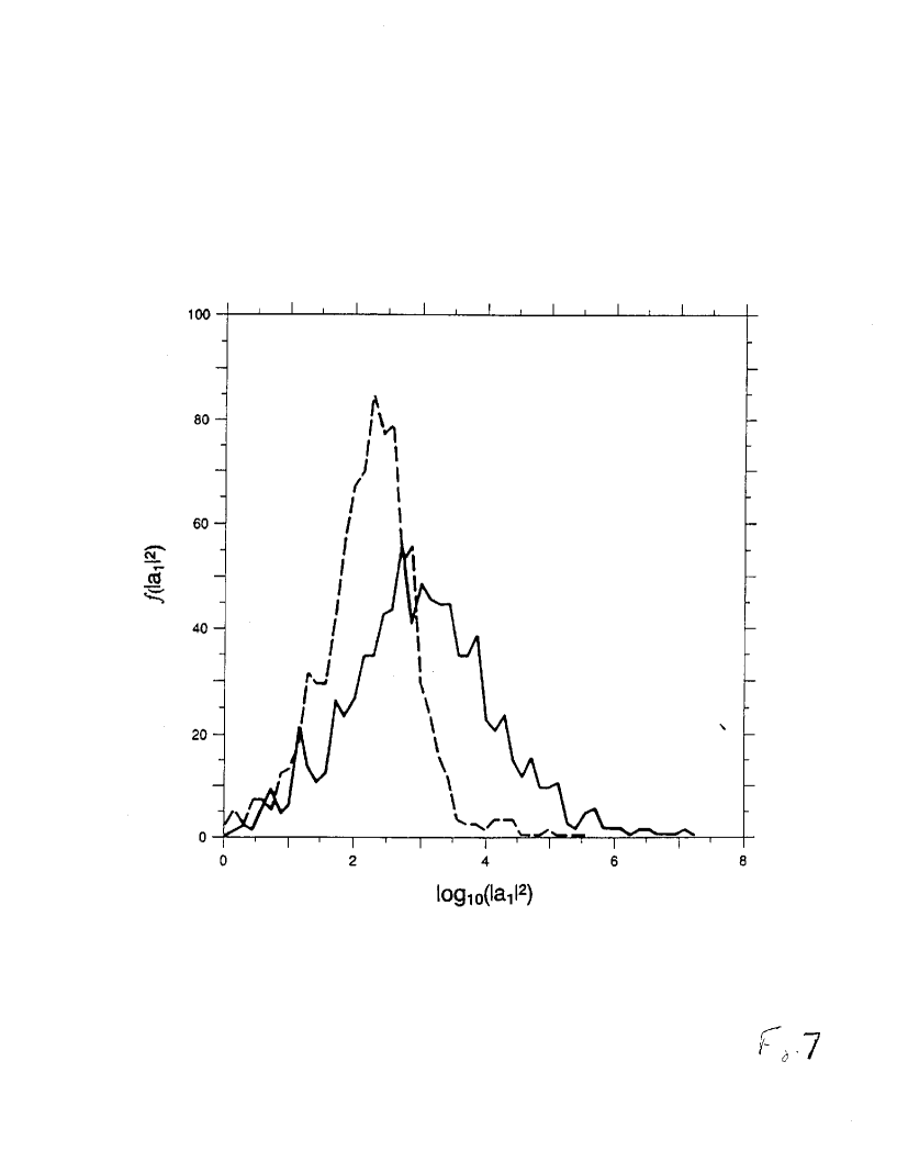
Figure 7: Numerically generated distribution of the intensity $\mid a_{1}\mid^{2}$ for the space-time problem with purely temporal bandwidth $\Delta\omega_{0}=10\gamma_{0}$ after an interval $\gamma_{0}\Delta t=45$. The solid curve has $\mid V_{1}/V_{2}\mid=16$ and the dashed curve has $\mid V_{1}/V_{2}\mid=100$. The abscissa is the base 10 logarithm of the intensity $\mid a_{1}\mid^{2}$.

In the space-time problem this factor of two also occurs for absolute instability driven by an incoherent pump when the decay wave group velocities are equal in magnitude and opposite in sign. We have verified our supposition by numerical integration that once again the distribution is broad for $\mid V_{1}\mid=\mid V_{2}\mid$ but is much narrower if $\mid V_{1}\mid>>\mid V_{2}\mid$ as shown in Fig. 7.

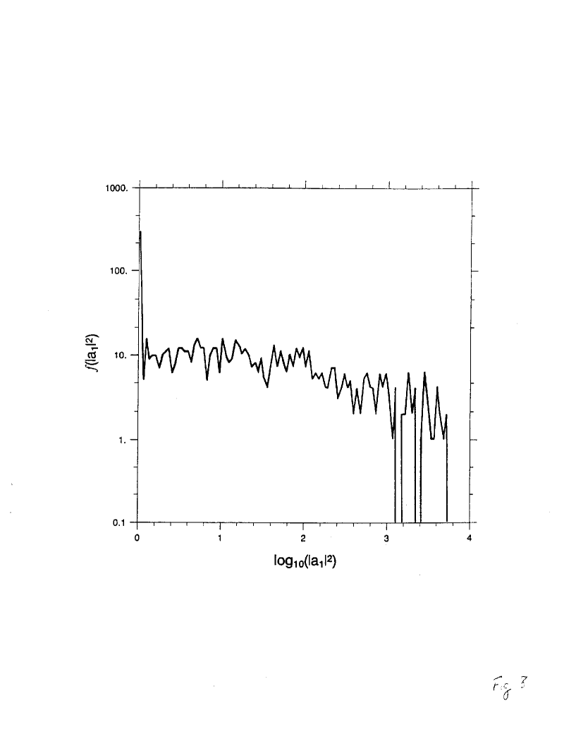
Figure 8: Numerically generated distribution of the intensity $\mid a_{1}\mid^{2}$ for a spatially incoherent pump with $\Delta k_{0}\mid\sqrt{\mid V_{1}V_{2}\mid}/\gamma_{0}=4,\nu_{1}=2\gamma_{0}$, $\nu_{2}=0$, and $V_{1}/V_{2}=-16$. The abscissa is the base 10 logarithm of the intensity $\mid a_{1}\mid^{2}$ after an interval $\gamma_{0}\Delta t=30$.

The validity of the RPA description in the intermediate domain was examined numerically in Sec. VII.B, by considering the model of a spatially incoherent pump driving a pair of decay waves satisfying the intermediate domain inequalities (VII.13). Although we did show that the RPA equations appear valid, we also discovered that the distribution of mode intensities (Fig. 8) is unusual in that it consists of a slowly decreasing tail on a distribution with a peak at nearly zero growth.

We also show in Sec. VII.C that the standard model of an ISI beam, Eq. (VII.15), which has both phase and intensity variation, can be treated as an incoherent pump wave provided the temporal and spatial bandwidth are large enough. Thus with the appropriate identification of experimental parameters with $\Delta\omega_{0}$ and $\Delta k_{0}$, the formulae in Sec. VI can be applied to experiments.[51-65]

A few remarks are in order regarding the derivation of the statistical equations that form the basics for the results outlined above.

The analysis begins in Section II with the completely nonlinear coupled-mode equations (II.2) appropriate for the case when the pump and decay waves are weakly coupled and weakly damped. In the linear analysis of this article, the pump wave is unaffected by the decay waves and the characteristic growth rate of the parametric instability is simply related to the pump amplitude at its mean wavevector (II.5). Normalization of the decay wave amplitudes to the average pump wave energy yields the linearized coupled-mode equation (II.7) in Fourier space. From these equations, the envelope equations (II.9) in Fourier space or (II.10) in real space are obtained by expanding the mode amplitudes about the value at the mean wavevector. These envelope equations are used in Sections III-V to obtain equations for the ensemble-averaged mode amplitudes and intensities.

If the pump wave has a distribution of wavevectors, then a given pair of decay waves will be frequency matched to only a portion of the pump wave spectrum. Thus one is naturally led to consider the frequency mismatches (III.1) for a general triplet of wavevectors or the mismatches (III.2) at the mean value of the decay wavevector. It is assumed that there exist triplets for which there is exact matching so that the mismatch near the mean wavevectors is small. The maximum value of the mismatches at the mean decay wavevector determines that the interaction is coherent if the mismatches are both small in the sense defined by III.6.

Two approaches to generating equations governing the ensemble averaged behavior of the instability are used in this article. The first employs the Bourret approximation[70] to obtain the dispersion relation (IV.5) and (IV.7) for the stability of the ensemble-averaged mode amplitude $<a_{j}>$. Each equation for $<a_{j}>$ is simple in that it does not involve the other but it does involve integrals over the spectral density of the pump wave and the frequency mismatch. In the incoherent limit or Markov limit defined by (IV.17), the dispersion relation takes the particularly simple and well- known form given by Eq. (IV.13) which states that the coupling between the waves is reduced by the ratio of the characteristic growth rate to the maximum mismatch $\Delta_{i~{}max}$ for $i\equiv 1,2$. For the one dimensional case with a pump spectrum that is Lorentzian, e.g. a Kubo-Anderson Process, the dispersion relations (IV.22) are the familiar ones derived previously[15-16] and the mismatch $\Delta_{i~{}max}$ is equivalent to the spectral widths $\Delta\omega_{i}$ defined by (IV.20) that are, within at most a factor of two, equal to the pump wave bandwidth $\Delta\omega_{0}$ (except for the special case of forward scatter where the $\Delta\omega_{1}<<\Delta\omega_{2}$). Note in one dimension, the problem of spatial and temporal incoherence are not independent in fact so our restriction to one dimension must yield the results[16] of Laval et al. However in our numerical models, this connection is broken for convenience and tractability.

The average amplitude equations (IV.5 and IV.7) are somewhat unsatisfying because $<a_{1}>$ and $<a_{2}>$ evolve independently. For the case of temporal incoherence alone, this untidiness was remedied by obtaining equations for the ensemble averaged intensities which are coupled and symmetric. Nevertheless, the result obtained for convective instabilities with only temporal incoherence is just that obtained by consideration of the most unstable average amplitude.

In Section V.B, the same procedure can be followed to obtain Bourret equations for the ensemble-averaged spectral densities (V.25) that are related to the mode intensities by (V.2). As with the amplitude equations (IV.5 and (IV.7), these equations involve integrals over the pump spectral density and the frequency mismatch; but, in addition, the integral contains the spectral density of the other decay wave at the pump shifted wavenumber. Two further approximations can be made: first, the Markov assumption valid provided that the mismatch is larger than the maximum of the growth rate and damping rates, i.e. ${\rm Min}(\Delta_{imax})>{\rm Max}(\gamma_{0},\nu_{j})$ removes the spatial and temporal growth rate from the integrand; second, the assumption that the decay wave spectral densities are slowly varying functions allows these densities to be evaluated at the mean wavenumber at exact matching. The first approximation yields the Random Phase Approximation (RPA) equations (V.28); and the subsidiary second approximation yields the set (V.32) with which the instability analysis is done in Section VI. As they must do, the RPA equations (V.28) are shown to reduce to the correct intensity equations derived using the Bourret approximation when the pump wave group velocity is infinite. For the purely temporal incoherence modeled by the Kubo-Anderson process[69], this latter result is exact.

Our conclusions are presented in Sec. VIII. There, we also give some examples of current interest and consider the special case when the temporal bandwidth is larger than one of the mode frequencies.

II The Coupled Mode Equations

II.1 The Coupled Mode Equations in Fourier Space.

In this article we limit our discussion to the coupling of three wave-packets which are both weakly coupled and weakly damped. We assume that each Fourier component $A_{k}^{i}$ of the wave packet i (with i = 0, 1, 2)) behaves in lowest order as a normal mode; i.e., it oscillates in time like ${\rm exp}(-i\omega_{k}^{i}t)$, where $\omega_{k}^{i}$ is the real part of the frequency $\Omega_{k}^{i}\equiv\omega_{k}^{i}-i\nu_{k}^{i}$ which characterizes the wave-packet i and which satisfies the dispersion relation $D_{i}(\Omega_{k}^{i},k)=0$. The assumption of weakly coupled and weakly damped modes can be written quantitatively as

$$\mid\omega_{k}^{i}\mid>>\nu_{k}^{i},\gamma$$

where $\nu_{k}^{i}$ is the linear damping increment of the Fourier component $A_{k}^{i}$, and where $\gamma$ denotes the inverse of the characteristic time for nonlinear evolution of the coupled modes. In this limit the equations describing the coupling of the three wave packets are of first order in time. In Fourier space they have the following general form:

$$\left[\partial_{t}+i\omega_{{\bf k}_{0}}^{0}+\nu_{{\bf k}_{0}}^{0}\right]A_{{\bf k}_{0}}^{0}=-\int d{\bf k}_{1}V_{{\bf k}_{0},{\bf k}_{1}}A_{{\bf k}_{1}}^{1}(A_{{\bf k}_{0}-{\bf k}_{1}}^{2})$$

$$\left[\partial_{t}+i\omega_{{\bf k}_{1}}^{1}+\nu_{{\bf k}_{1}}^{1}\right]A_{{\bf k}_{0}}^{0}=\int d{\bf k}_{0}V_{{\bf k}_{0},{\bf k}_{1}}A_{{\bf k}_{0}}^{0}(A_{{\bf k}_{0}-{\bf k}_{1}}^{2})^{*}$$

$$\left[\partial_{t}+i\omega_{{\bf k}_{2}}^{2}+\nu_{{\bf k}_{2}}^{2}\right]A_{{\bf k}_{2}}^{2}=\int d{\bf k}_{0}V_{{\bf k}_{0},{\bf k}_{0}}A_{{\bf k}_{0}}^{0}(A_{{\bf k}_{0}-{\bf k}_{2}}^{1})^{*}$$

where $A_{{\bf k}_{0}}^{i}$ is proportional to the Fourier component of the electric field of wave i; wave 0 refers to the pump wave and waves 1 and 2 to the decay waves. The coupling constants $V_{{\bf k}_{0},{\bf k}_{1}}$ are derived from the usual field expansion of the fluid or the Vlasov equations.

The parametric approximation consists in neglecting the RHS of Eq. (II.2a) and in taking $A_{{\bf k}_{0}}^{0}=A_{{\bf k}_{0}}^{0}{\rm exp}(-i\omega_{{\bf k}_{0}}^{0}t$) in the RHS of Eqs. II.2b and II2c. In this limit the latter equations describe correctly the parametric coupling of waves in the usual decay regime (the so-called modified decay instability and the modulational instability[76] cannot be described by these equations since they correspond to coupled mode equations in which the second order partial derivative in time must be retained).

In this article we derive the conditions for a reduction of the parametric growth due to the pump wave incoherence. The incoherence of the pump wave may be either temporal, or spatial, or both. In the case of purely temporal incoherence, the wave-numbers $k_{0}$ of the different components of the pump wave all have the same direction; if $\Delta\omega_{0}$ is the spectral width in frequency space of the pump wave and is small compared to the pump frequency, $\Delta\omega_{0}<<\omega_{0}$, the spread $\Delta K_{0}$ of the corresponding wave-number modulus $k_{0}\equiv\mid k_{0}\mid$ is given by

$$\Delta k_{0}\simeq\Delta\omega_{0}/V_{g0}$$

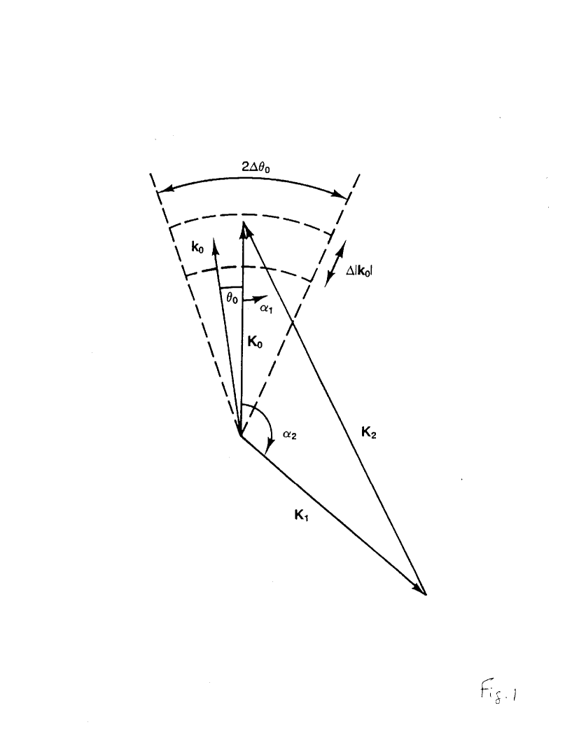
Figure 1: Geometry of the scattering: $K_{0},K_{1},K_{2}$ are the mean wavenumbers of the pump wave and of the decay waves; the pump wave vector $K_{0}$ varies in magnitude an amount $\Delta\mid k_{0}\mid$ and lies in a cone of angle $\Delta\theta_{0}$ about the direction of the mean, $K_{0}$. Also shown are the angles $\alpha_{2}$ and $\alpha_{1}$ which the mean wavevectors $K_{1}$ and $K_{2}$ make with the mean pump wavevector $K_{0}$

Here ${\bf V}_{g0}$ is the characteristic group velocity of the pump wave and $V_{g0}$ denotes $V_{g0}\equiv\mid{\bf V}_{g0}\mid$. In the case of purely spatial incoherence, all the wave-numbers ${\bf k}_{0}$ have the same modulus $k_{0}\equiv\mid{\bf k}_{0}\mid$ and are spread within a small cone, the half angle of aperture of the latter being denoted by $\Delta\Theta_{0}$. In the general case, the mean wave-number and frequency of the pump wave are denoted by ${\bf K}_{0}$ and $\omega_{0}\equiv\omega_{{\bf K}_{0}}^{0}$ respectively, and the incoherence of the pump wave is characterized by the spectral width $\Delta k_{0}=\omega_{0}/V_{g0}$ and by the half-angle spread $\Delta\Theta_{0}$. We will assume an azimuthal symmetry around ${\bf K}_{0}$ and a cross section of the total domain of existence of ${\bf k}_{0}$ is displayed in Fig. 1.

An assumption made implicitly when using Eqs. (II.2) to investigate the incoherence effects is that the spread in frequency $\Delta\omega_{0}$ is much smaller than the frequencies $\omega_{k_{i}}^{i}$ of the various waves. Similarly, the spread in wave number $\mid\Delta{\bf k}_{0}\mid\sim\Delta\omega_{0}/V_{g0}+K_{0}\Delta\Theta_{0}$ is assumed to be small compared to wave numbers $\mid{\bf k}_{i}\mid$.

We denote by $\alpha_{2}$ the angle between the propagation directions of the pump wave and of the wave 1. For a given direction $\alpha_{2}$ of the wave 1, there is a unique couple $({\bf K}_{1},\omega_{{\bf K}_{1}}^{1}),({\bf K}_{2},\omega_{{\bf K}_{2}}^{2})$ satisfying the two resonance conditions,

$$\omega_{{\bf K}_{0}}^{0}=\omega_{{\bf K}_{1}}^{1}+\omega_{{\bf K}_{2}}^{2},$$

$${\bf K}_{0}={\bf K}_{1}+{\bf K}_{2}.$$

Throughout this article we investigate the reduction of the parametric instability corresponding to a given direction $\alpha_{2}$ and the capital letters ${\bf K}_{1}$ will be used exclusively for this wavenumber of wave i which corresponds to the resonance conditions (II.4), for i = 1, 2; as stated before, ${\bf K}_{0}$ denotes the mean wavenumber of the pump wave, and the symbol ${\bf k}_{0}$ will denote a generic wavenumber of the pump wave; lastly $\alpha_{1}$ is the angle between the mean pump wave-number ${\bf K}_{0}$ and the wave number ${\bf K}_{2}$ corresponding to the resonance conditions II.4 written for an angle $\alpha_{2}$.

We may now relate the characteristic growth rate of the parametric instability corresponding to the coherent case, $\gamma_{0}$, for a given angle of observation $\alpha_{2}$, to the mode coupling constants and the pump amplitude by

$$\gamma_{0}^{2}=\mid V_{{\bf K}_{0},{\bf K}_{1}}\mid^{2}\langle\mid A_{0}\mid^{2}\rangle$$

where $\langle\mid A_{0}\mid^{2}\rangle$ denotes the average energy of the pump wave in a sense defined in the next section.

Defining the dimensionless coupling constants and wave amplitudes by

$$v_{{\bf k}_{0},{\bf k}_{1}}\equiv V_{{\bf k}_{0},{\bf k}_{1}}/V_{{\bf K}_{0},{\bf K}_{1}}$$

$$a_{{\bf k}_{\alpha}}^{\alpha}\equiv A_{{\bf k}_{\alpha}}^{\alpha}/<\mid A_{0}\mid^{2}>^{1/2}$$

The dimensionless form of equations is simply

$$\left[\partial_{t}+i\omega_{{\bf k}_{1}}^{1}+\nu_{{\bf k}_{1}}^{1}\right]a_{{\bf k}_{1}}^{1}=\gamma_{0}\int d{\bf k}_{0}v_{{\bf k}_{0},{\bf k}_{1}}a_{{\bf k}_{0}}^{0}\left(a_{{\bf k}_{0}-{\bf k}_{1}}^{1}\right)^{*}$$

$$\left[\partial_{t}+i\omega_{{\bf k}_{2}}^{2}+\nu_{{\bf k}_{2}}^{2}\right]a_{{\bf k}_{2}}^{2}=\gamma_{0}\int d{\bf k}_{0}v_{{\bf k}_{0},{\bf k}_{0}-{\bf k}_{2}}a_{{\bf k}_{0}}^{0}\left(a_{{\bf k}_{0}-{\bf k}_{2}}^{1}\right)^{*}$$

where $v_{{\bf k}_{0},{\bf k}_{\alpha}}$ is a slowly varying function of ${\bf k}_{0}$ and ${\bf k}_{\alpha}$, with $v_{{\bf K}_{0},{\bf K}_{\alpha}}=1$. Finally, the latter equations are supplemented by the following equation for the pump wave amplitude

$$a_{{\bf k}_{0}}^{0}=a_{{\bf k}_{0}}^{0}{\rm exp}(-i\omega_{{\bf k}_{0}}^{0}t)$$

II.2 The Envelope Approximation for the Coupled Mode Equations in Real Space

At this point we can make a connection between the coupled mode equations (II.7) written in their general form in Fourier space and their so-called envelope equation form in real space. The envelope approximation for the coupled mode equations corresponds to the first order expansion of $\omega_{{\bf k}_{i}}^{i}$ in a power series of (${\bf k}_{i}-{\bf K}_{i}$). By writing $\omega_{{\bf k}_{i}}^{i}\simeq\omega_{{\bf K}_{i}}^{i}+({\bf k}_{i}-{\bf K}_{i})\cdot{\bf V}_{gi}$, and by setting

$$a_{{\bf k}_{i}}^{i}=\hat{a}_{{\bf k}_{i}-{\bf K}_{i}}^{i}{\rm exp}(-i\omega_{{\bf K}_{i}}^{i}t)$$

or i = 1 and 2, and

$$a_{{\bf k}_{0}}^{0}=\hat{a}_{{\bf k}_{0}-{\bf K}_{0}}^{0}{\rm exp}\left(-i[\omega_{{\bf K}_{0}}^{0}+({\bf k}_{0}-{\bf K}_{0})\cdot{\bf V}_{g0}]t\right)$$

the coupled mode equations can be written as

$$\left(\partial_{t}+i{\bf k}_{1}^{\prime}\cdot{\bf V}_{g1}+\nu_{1}\right)\hat{a}_{{\bf k}_{1}^{\prime}}=\gamma_{0}\int d{\bf k}_{0}^{\prime}\hat{a}_{{\bf k}_{0}^{\prime}}^{0}\left(\hat{a}^{2}\right)^{*}_{{\bf k}_{0}^{\prime}-{\bf k}_{1}^{\prime}}{\rm exp}-i\left({\bf k}_{0}^{\prime}\cdot{\bf V}_{g0}\right)t$$

$$\left(\partial_{t}+i{\bf k}_{2}^{\prime}\cdot{\bf V}_{g2}+\nu_{2}\right)\hat{a}_{{\bf k}_{2}^{\prime}}=\gamma_{0}\int d{\bf k}_{0}^{\prime}\hat{a}_{{\bf k}_{0}^{\prime}}^{0}\left(\hat{a}^{1}\right)^{*}_{{\bf k}_{0}^{\prime}-{\bf k}_{2}^{\prime}}{\rm exp}-i\left({\bf k}_{0}^{\prime}\cdot{\bf V}_{g0}\right)t$$

where ${\bf k}_{i}^{\prime}={\bf k}_{i}-{\bf K}_{i}$ and we neglected the slow variation of $\nu_{{\bf K}_{1}+{\bf k}_{i}^{\prime}}$ and of $v_{{\bf K}_{0}+{\bf k}_{0}^{\prime},{\bf K}_{1}+{\bf k}_{1}^{\prime}}$ with ${\bf k}_{1}^{\prime}$ and ${\bf k}_{0}^{\prime}$. By taking the inverse Fourier transforms of Eqs. II.9, one obtains the mode-coupling equations in their envelope approximation limit, namely

$$\left(\partial_{t}+{\bf V}_{g1}\cdot\partial_{\bf x}+\nu_{1}\right)a_{1}({\bf x},t)=\gamma_{0}S\left({\bf x}-{\bf V}_{g0}t\right)a_{2}^{*}$$

$$\left(\partial_{t}+V_{g2}\cdot\partial_{x}+\nu_{2}\right)a_{2}({\bf x},t)=\gamma_{0}S\left({\bf x}-{\bf V}_{g0}t\right)a_{1}^{*}$$

where the quantity $S({\bf x}-{\bf V}_{g0}t)$ is defined by

$$S({\bf x}-{\bf V}_{g0}t)=\int d{\bf k}_{0}^{\prime}a_{{\bf k}_{0}^{\prime}}{\rm exp}(i{\bf k}_{0}^{\prime}\cdot({\bf x}-{\bf V}_{g0}t))$$

Equations II.10 are the envelope equations which have been investigated with the statistical methods described in the next section. These equations are generalizations to three dimensions of one dimensional equations used in previous treatments of this subject[16]. For the sake of simplicity the envelope approximation will henceforth refer to either the coupled mode equations written in their envelope form II.9, or the first order expansion of $\omega_{k_{i}}^{i}$.

Concerning our notation, ${\bf V}_{g\alpha}({\bf k}_{\alpha})$ will denote, in the following the group velocity corresponding to a generic wavenumber ${\bf k}_{\alpha}$, namely ${\bf V}_{g\alpha}({\bf k}_{\alpha})\equiv(\partial\omega^{\alpha}_{{\bf k}\alpha}/\partial{\bf k}_{\alpha})$; the notation $V_{g\alpha}$ will be reserved to the case of exact resonance, i.e., ${\bf V}_{g\alpha}\equiv{\bf V}_{g\alpha}({\bf K}_{\alpha})$.

On the other hand, the quantity $a_{\alpha}$ (x,t) will denote the Fourier transform of the field $a_{{\bf k}_{\alpha}}^{(\alpha)}(t)$ in the case where one considers the mode coupling equations in their general form (II.7); the notations $\hat{a}_{\alpha}(x,t)$ and $\hat{a}_{k_{\alpha}^{\prime}}^{(\alpha)}$ will be used by contrast in the case where the fast time and space variations have been factorized ab initio as in Eq. (II.8a). The connection between the two sets is given by

$$\hat{a}_{{\bf k}_{\alpha}^{1}}^{(\alpha)}\equiv a_{{\bf K}_{\alpha}+{\bf k}_{\alpha}^{\prime}}{\rm exp}(+i\omega_{{\bf K}_{\alpha}}^{(\alpha)}t)$$

and

$$a_{\alpha}(x,t)=\hat{a}_{\alpha}(x,t){\rm exp}~{}i({\bf K}_{\alpha}\cdot{\bf x}-\omega_{{\bf K}_{\alpha}}^{(\alpha)}t)+c.c.$$

III Statistical Description for Coupled Mode Equations

III.1 The Frequency Mismatches

In the two following sections, we derive equations describing the evolution of average quantities such as the average amplitude $\langle a_{\alpha}\rangle$, or the average intensity $\langle\mid a_{\alpha}\mid^{2}\rangle$ of wave $\alpha$. Here $<\phi>$ denotes the statistical average of the physical quantity $\phi$, and its fluctuation is written as $\delta\phi\equiv\phi-<\phi>$. The meaning of a statistical average can in some sense be understood as a time average, and the use of a statistical framework is justified for the following reasons: a reduction of the parametric growth can be expected whenever the spectral width $\mid\mid\Delta{\bf k}_{0}\mid\mid$ of the pump wave is large enough (due to a temporal or spatial incoherence) for its correlation time - as seen by the decay waves, in a sense to be defined in this section - to be shorter than the other characteristic times, namely, the damping and the growth time, $\nu_{\alpha}^{-1}$ and $\gamma_{0}^{-1}$. In this case, the statistical description is justified whenever the correlation length in K-space of the pump wave $a_{{\bf k}_{0}}^{(0)}$ is small compared to its spectral width (e.g., when the number of ISI echelons or phase elements is large). In this limit the pump wave electric field can indeed be regarded as a stochastic process with a short correlation time and the standard statistical techniques can be applied. In the case of a purely temporal incoherence, the statistical description is physically justified only if the pump wave bandwidth is caused by some stochastic process, e.g., the spread over several independent lines of a non-monochromatic laser. Similarly, in the case of a purely spatial incoherence, the natural spread in angle of the pump wave wavenumbers must follow from the sum of many independent beamlets. Such a statistical independence may result from a random phase shift given to the different beamlets by means of a transparent phase mask[3]; it may also be due to the scattering of the incident pump wave upon static random fluctuations. Lastly such a spatial incoherence can be achieved in the so-called ISI technique[2] by a combination of delay increments $\Delta t$ given to the beamlets by echelon structures and of the laser temporal incoherence in the case $\Delta\omega_{0}\Delta t\geq 1$. In these techniques, the laser beam is broken up into a number of statistically independent ”beamlets” that are brought to focus by an optic of f-number, $f_{\#}$. In the focal plane these beamlets overlap creating a spatially nonuniform pattern with coherence length across the beam $X_{c}=\pi/(k_{0}{\sin}\theta_{f})$ where $\theta_{f}$ is the half-angle of the optic, i.e. $\theta_{f}\simeq(2f_{\#})^{-1}$.

We will henceforth restrict ourselves to physical situations where the statistical independence between the pump wave Fourier components is satisfied; the pump wave electric field will thus be regarded as a stochastic variable with zero mean; its statistical properties will be assumed to be entirely determined by its spectral density denoted as $n_{{\bf k}_{0}}^{(0)}$, the latter being itself characterized by its spectral width $\Delta{\bf k}_{0}$, that is to say by $\Delta k_{0}=\mid\Delta{\bf k}_{0}\mid=\Delta\omega_{0}/{\bf V}_{g0}$ (temporal incoherence) and $\Delta\theta_{0}$ (spatial incoherence).

Before deriving the statistical equations for the time evolution of $<a_{i}>$ or $<\mid a_{i}\mid^{2}>$, let us first consider on a physical basis the reduction of the parametric growth caused by the pump wave incoherence. Suppose that we consider the parametric coupling corresponding to a given angle $\alpha_{2}$ between the pump wave and the first decay wave direction; this angle defines the resonant wavenumbers $K_{1}$ and $K_{2}$ of the decay waves corresponding to the exact resonance condition II.3 with the mean pump wave number ${\bf K}_{0}$. If one considers now a generic wavenumber ${\bf k}_{0}\not={\bf K}_{0}$ of the pump wave, the resonance conditions II.3 can no longer be satisfied for the same wave-numbers ${\bf K}_{1}$ and ${\bf K}_{2}$. One is thus led to define the resonance mismatches $\Delta_{1}$ and $\Delta_{2}$ as

$$\Delta_{1}({\bf k}_{0},{\bf k}_{2})\equiv\omega_{{\bf k}_{0}}^{(0)}-\omega_{{\bf k}_{0}-{\bf k}_{2}}^{(1)}-\omega_{{\bf k}_{2}}^{(2)}$$

and

$$\Delta_{2}({\bf k}_{0},{\bf k}_{1})\equiv\omega_{{\bf k}_{0}}^{(0)}-\omega_{{\bf k}_{1}}^{(1)}-\omega_{{\bf k}_{0}-{\bf k}_{1}}^{(2)}$$

When discussing the effect of the pump incoherence in the case of a given geometry defining the resonant wave numbers $K_{1}$ and $K_{2}$, it is sufficient to consider the quantities $\Delta_{1}({\bf k}_{0},{\bf K}_{2})$ and $\Delta_{2}({\bf k}_{0},{\bf K}_{1})$. In order to simplify our notation, we will denote in our paper by $\overline{\theta}$ the value of a quantity ${\overline{\theta}}$ in the case of the exact resonance ${\bf k}_{1}={\bf K}_{1}$ and ${\bf k}_{2}={\bf K}_{2}$. Accordingly we define $\overline{\Delta}_{1}({\bf k}_{0})$ and $\overline{\Delta}_{2}({\bf k}_{0})$ by

$$\overline{\Delta}_{1}({\bf k}_{0})\equiv\Delta_{1}({\bf k}_{0},{\bf K}_{2})$$

$$\overline{\Delta}_{2}({\bf k}_{0})\equiv\Delta_{2}({\bf k}_{0},{\bf K}_{1})$$

In the case of an incoherent pump wave, the spectral width $\Delta{\bf k}_{0}$ gives rise to a characteristic size for $\overline{\Delta}_{i}({\bf k}_{0})$, which will be denoted as $\Delta_{i{\rm max}}$, i.e.

$$\Delta_{i~{}{\rm max}}=\overline{\Delta}({\bf K}_{0}+\Delta{\bf k}_{0})$$

For instance, in the case where the envelope approximation can be applied, one readily finds $\Delta_{1~{}{\rm max}}=({\bf V}_{g0}-{\bf V}_{g1})\cdot\Delta{\bf k}_{0}$ which can also be written as

$$\Delta_{1~{}{\rm max}}=\mid(V_{g0}-V_{g1}{\rm cos}~{}\alpha_{2})\Delta{\bf k}_{0}-K_{0}V_{g1}{\rm sin}~{}\alpha_{2}\Delta\Theta_{0}\mid$$

or

$$\Delta_{1{\rm max}}=\mid(1-V_{g1}{\rm cos}~{}\alpha_{2}/V_{g0})\Delta\omega_{0}-K_{0}V_{g1}{\rm sin}~{}\alpha_{2}\Delta\Theta_{0}\mid$$

More generally, it has been shown[7] that it is sufficient to expand $\Delta_{1~{}{\rm max}}$ as follows:

$$\Delta_{1max}=\mid t_{1}\Delta k_{0}+\sigma_{1}\Delta\Theta_{0}+\beta_{1}\Delta\Theta_{0}^{2}\mid$$

with $t_{1}=(V_{g0}-V_{g1}{\rm cos}\alpha_{2}),\sigma_{1}=-V_{g1}K_{0}{\rm sin}\alpha_{2}$. For backscatter, $\sigma_{1}$ vanishes and it is necessary to expand to second order in $\Delta\Theta_{0}$. The coefficient of $\Delta\Theta_{0}^{2},\beta_{1},$ can be computed in terms of the waves parameters $\partial\omega^{\alpha}/\partial{\bf K}_{j}$, and $\partial^{2}\omega^{\alpha}/\partial{\bf K}_{i}\partial{\bf K}_{j}^{1}$, and the angles $\alpha_{i}$ defining the geometry of the interaction. The first term in (III.5) corresponds to temporal incoherence and the last two to spatial incoherence.

In the present article, we will mainly restrict ourselves to some particular examples convenient for numerical experiments, in which the 2D character of the pump wave incoherence is modeled by the introduction of two parameters $\Delta\omega_{0}$ and $\Delta k_{0}$, playing the role of the temporal and spatial incoherence, respectively, so that $\Delta_{i~{}{\rm max}}$ is similarly written as $\Delta_{i~{}{\rm max}}=\alpha_{i}\Delta\omega_{0}+\beta_{i}\Delta k_{0}$.

Regarding now under which conditions the pump wave incoherence modifies the parametric coupling, one may first easily admit that a sufficient condition for neglecting the pump wave incoherence is that the two following inequalities be both satisfied:

$$\Delta_{1max}<\mid D_{1}\mid$$

$$\Delta_{2max}<\mid D_{2}\mid$$

In the latter inequalities, $D_{i}$ denotes the dispersion relation

$$D_{i,{\bf k}_{i}}\left(\gamma,k\right)\equiv\gamma+i\left(\omega_{{\bf k}_{i}+i\kappa}^{(i)}-\omega_{{\bf k}_{i}^{(i)}}\right)+\nu_{i}$$

In the envelope approximation, $D_{i}$ reduces to

$$\hat{D}_{i,~{}{\bf k}_{i}}\left(\gamma,k\right)\equiv\gamma-\kappa\cdot{\bf V}_{gi}\left({\bf k}_{i}\right)+\nu_{i}$$

where, $\gamma$ and $\kappa$ denote the time and space growth rates. (It can be noted that our definitions of $D_{i}$ and $\hat{D}_{i}$ are consistent with each other, in the sense that if one considers ab initio the coupled mode equations in their envelope form (II.10), $D_{i}$ reduces identically to $\hat{D}_{i}$ without any further approximation: in this case, one has indeed $\omega_{{\bf\kappa}_{i}}^{(i)}={\bf\kappa}_{i}\cdot{\bf V}_{gi}$, from which the relation $D_{i}=\hat{D}_{i}$ follows.)

Concerning the inequalities (III.6), we will see more generally that the coherent or incoherent character of the parametric coupling is controlled by inequalities between $\Delta_{imax}$ and $\mid D_{j}\mid$. On the other hand, since $\gamma$ and $\kappa$ are related through the dispersion relation, the size of $D_{j}$ depends upon the nature of the instability which is considered, namely convective, absolute, or spatially amplifying. It therefore follows that the coherent or incoherent character of the parametric coupling depends itself on the nature of the instability. Defining now as ”incoherent” the domain where the pump wave incoherence induces a reduction of the parametric growth, one realizes that such a domain should be specified as ”convectively incoherent”, or ”absolutely incoherent”, or ”incoherent for spatial amplification”. For instance, in the case of a purely temporal incoherence, with $V_{g0}=\infty$, it has been shown in (Laval, et.al.) that the pump wave incoherence reduces the convective growth for $\Delta\omega_{o}>{\rm Max}\left(\nu_{1},\nu_{2}\right)$ and $\Delta\omega_{0}>\gamma_{0}$, whereas in the case of an absolute instability, the absolute growth can be reduced only if $\Delta\omega_{0}$ satisfies:

$$\Delta\omega_{0}>\gamma_{0}\mid{V_{1}\over V_{2}}\mid^{1/2}>\nu_{2}\mid{V_{1}\over V_{2}}\mid.$$

[For simplicity we consider the case where $\mid V_{1}\mid>>\mid V_{2}\mid$ and $\nu_{2}/\mid V_{2}\mid>>\nu_{1}/\mid V_{1}\mid$.] One thus sees with this simple case that the reduction of the absolute growth is much more difficult to achieve than that of the convective growth.

We may recall here that the convective growth rate characterizes the instability in the early stage of its development, by contrast with its long time evolution which is characterized either by the absolute growth rate (whenever the conditions for their existence are satisfied) or by the spatial amplification growth length (in the opposite case).

In this article we will derive the conditions under which the pump incoherence gives rise to a reduction of the convective and of the absolute growth rates and an increase in the spatial amplification length. It will be found that generally the conditions for reducing the absolute instabilities are more severe than those for the convective ones. For this reason we will concentrate mainly our discussions on the ”convectively incoherent” domain, which may thus be regarded as the largest domain in which a reduction of the parametric growth may be expected in the early stage of the instability development. In order to simplify our terminology, the ”incoherent” domain, without any other specification, will henceforth refer to the previously defined ”convectively incoherent” domain.

Restricting ourselves to the convective instabilities, one may rewrite inequalities (III.6) as:

$$\Delta_{1max}<\nu_{1},\gamma_{0}$$

$$\Delta_{2max}<\nu_{2},\gamma_{0}$$

in which we used $\gamma\sim\gamma_{0}$ in the coherent regime. As said before, these inequalities represent only a sufficient condition for the pump wave incoherence being ignorable; the question is thus whether both of these two inequalities have to be satisfied, or only one. In order to answer this question, we first introduce in a brief discussion the validity conditions of the statistical equations which describe the time evolution of the quantities $<a_{i}>$ and $<\mid a_{i}\mid^{2}>$.

III.2 The Incoherent and RPA domains

A statistical description for the evolution of the decay waves 1 and 2 is provided by the Random Phase Approximation (RPA) equations for the evolution of the average intensities $<a_{i}a_{i}^{*}>$. The latter provide equations for the evolution on a slow time - or slow space - scale of the spectral densities $n_{k}^{(i)}$(x,t) of the decay waves [the latter functions $n_{\bf k}^{(i)}$(x,t)] will be defined in the general case by Eq. (V.2); at this point it is sufficient to say that for a purely temporal problem one has the usual relation $<a_{\bf k}^{(i)}(a_{{\bf k}^{\prime}}^{(i)})^{*}>=\delta({\bf k}-{\bf k}^{\prime})n_{k}^{(i)}$]. The RPA equations are nonlinear and they may account for the pump depletion; the interested reader is referred to standard textbooks[72] for their derivation in the general case. In our problem of stability analysis, we face a linear problem; we could naturally use directly the RPA equations on which we would make a posteriori the linear approximation which consists in neglecting the pump depletion. In this article we will follow a different route. We will first take advantage of the linear character of the coupled mode equations II.6 which will enable us to use the so-called Bourret approximation[70] for the evolution of $<a_{i}>$; on the other hand, the Bourret approximation for the evolution of the intensities $<a_{i}a_{i}^{*}>$ is easily tractable within the envelope approximation only, and then only for the special case where the pump wave group velocity $V_{g0}$ is infinite. In the general case it is necessary to make supplementary approximations to the Bourret equations, and these approximations are justified in a domain that will be defined subsequently as the ”RPA domain.”

Returning now to the condition defining the domain in which the parametric coupling takes place coherently, we first define the temporal and spatial growth rates $\gamma_{<a_{i}>},{\bf\kappa}_{<a_{i}>},$ for $\langle\mid a_{i}\mid^{2}\rangle$, and $\gamma_{\langle a^{2}\rangle},{\bf\kappa}_{\langle a^{2}\rangle}$ for $\langle\mid a_{i}\mid^{2}\rangle$, according to:

$$\langle\hat{a}_{i}({\bf x},t)\rangle=a_{{\bf K}_{i}}^{(i)}(0)\,{\rm exp}\left[\gamma_{\langle a_{i}\rangle}t-{\bf\kappa}_{\langle a_{i}\rangle}\cdot{\bf x}\right]$$

$$\langle\mid\hat{a}_{i}\mid^{2}(x,t)\rangle=\mid a_{{\bf K}_{i}}^{(i)}\mid^{2}(0)\,{\rm exp}~{}2\left[\gamma_{\langle a^{2}\rangle}t-{\bf\kappa}_{\langle a^{2}\rangle}\cdot{\bf x}\right]$$

A factor 2 has been included in the argument of the exponential defining $\gamma_{<a^{2}>}$ and $\kappa_{<a^{2}>}$ so that the equality $\gamma_{<a>}=\gamma_{<a^{2}>}$ holds in the coherent case. More generally the Schwartz inequality yields the following result

$$\gamma_{\langle a^{2}\rangle}\geq\gamma_{\langle a_{i}\rangle}$$

for i = 1 and 2, in the case of a purely temporal growth (and $\mid\mid{\bf\kappa}_{\langle a^{2}\rangle}\mid\mid\geq\mid\mid{\bf\kappa}_{\langle a_{i}\rangle}\mid\mid$ in the case of a spatial growth).

Admitting that the pump incoherence may only reduce the parametric growth (in the case of a convective instability in a homogeneous plasma), one realizes that, whenever either $\langle a_{1}\rangle$ or $\langle a_{2}\rangle$ behaves coherently, the two quantities $<\mid a_{1}\mid^{2}>$ and $<\mid a_{2}\mid^{2}>$ must also behave both coherently.

In the next section, it will be found that there exists a growth reduction for $<a_{1}>$ only if the mismatch $\Delta_{2~{}{\rm max}}$ satisfies the condition $\Delta_{2~{}{\rm max}}>(\nu_{2},\gamma_{0})$. From the previous considerations, it follows that the wave energies $<\mid a_{i}\mid^{2}>$ will behave coherently whenever at least one of the two following inequalities is satisfied:

$$\Delta_{1~{}{\rm max}}<{\rm Max}(\nu_{1},\gamma_{0})$$

or

$$\Delta_{2~{}{\rm max}}<{\rm Max}(\nu_{2},\gamma_{0})$$

These inequalities define what is referred to henceforth as the ”convectively coherent” domain. Accordingly, the ”convectively incoherent” domain - or simply incoherent domain - is defined by the two conditions

$$\Delta_{1~{}{\rm max}}>{\rm Max}(\nu_{1},\gamma_{0})$$

and

$$\Delta_{2~{}{\rm max}}>{\rm Max}(\nu_{2},\gamma_{0})$$

On the other hand, the validity conditions for the RPA are very stringent. In Section V they will be found to consist of two sets of inequalities; the first one corresponds to the inequalities opposite to (III.6), namely

$$\Delta_{1~{}{\rm max}}>{\rm Max}\mid D_{1}\mid$$

$$\Delta_{2~{}{\rm max}}>{\rm Max}\mid D_{2}\mid$$

and a second set involving the cross inequalities

$$\Delta_{1~{}{\rm max}}>{\rm Max}\mid D_{2}\mid$$

$$\Delta_{2~{}{\rm max}}>{\rm Max}\mid D_{1}\mid$$

Since the RPA dispersion relation yields $\gamma_{\langle a^{2}\rangle}\sim\gamma_{0}^{2}/{\rm min}(\Delta_{i~{}{\rm max}})$ for the convective growth rate, the latter inequalities reduce essentially to

$$\Delta_{1~{}{\rm max}}>{\rm Max}(\nu_{1},\gamma_{0})$$

$$\Delta_{2~{}{\rm max}}>{\rm Max}(\nu_{2},\gamma_{0})$$

$$\Delta_{1~{}{\rm max}}>{\rm Max}(\nu_{2},\gamma_{0})$$

$$\Delta_{2~{}{\rm max}}>{\rm Max}(\nu_{1},\gamma_{0})$$

which can also be recast into the more compact form

$${\rm Min}(\Delta_{j~{}{\rm max}})>{\rm Max}(\nu_{i},\gamma_{0})$$

The latter inequalities (III.14) or (III.15), define what is called the (convective) RPA domain.

One can now see that the incoherent domain (III.12) is subdivided into 1) the RPA domain in which the cross inequalities (III.14b) and (III.14d) are both satisfied, 2) the intermediate domain corresponding to the regime where the two inequalities $\Delta_{1~{}{\rm max}}>(\nu_{1},\gamma_{0})$ and $\Delta_{2max}>(\nu_{2},\gamma_{0})$ are both fulfilled whereas at least one of the cross inequalities (III.14c) and (III. 14d) is not satisfied.

In this intermediate domain there is no theory which is easily tractable for an explicit computation of the growth rate of the average energy $<\mid a_{\alpha}\mid^{2}>$. On the other hand, the Bourret approximation makes it possible to calculate the growth rate of the average amplitudes $<a_{1}>$ and $<a_{2}>$: it will then be found in Section V that the larger growth rate of $\gamma_{<a_{1}>}$ and $\gamma_{<a_{2}>}$ is given (for the convective instabilities), by the RPA prediction $\gamma^{RPA}$ for $<\mid a_{1}\mid^{2}>$ and $<\mid a_{2}\mid^{2}>$ within a numerical factor no larger than two.

For this reason we will argue in Section VI that although the RPA equations are not in their range of applicability in the intermediate domain, the convective growth rate $\gamma_{<a^{2}>}$ for the intensities remains of the order of $\gamma^{RPA}$. Accordingly, in the whole incoherent domain defined by the two inequalities:

$$\Delta_{1~{}{\rm max}}>{\rm Max}(\nu_{1},\gamma_{0})$$

and

$$\Delta_{2~{}{\rm max}}>{\rm Max}(\nu_{2},\gamma_{0})$$

the convective growth rate $\gamma_{<a^{2}>}$ can be approximated by the RPA prediction $\gamma^{RPA}$. The latter approximation is one of the main results of our paper since it makes it possible to compute the reduction of the parametric growth induced by the pump wave incoherence from the simple calculation of the RPA coupling constants $\gamma_{11}^{RPA}$ and $\gamma_{22}^{RPA}$.

IV The Bourret Approximation for the Average Amplitudes

IV.1 Introduction to the Bourret Approximation

The Bourret approximation[69,70] is a well known equation in the context of propagation in random media; it deals with stochastic linear multiplicative equations of the form

$$\left(\partial_{t}+L_{0}\right)A=\gamma_{0}SA$$

where $L_{0}$ is a linear deterministic operator, S a linear stochastic operator with zero mean, $<S>=0$, and A is the physical quantity of interest. The Bourret approximation can be simply derived as follows:

• by averaging Eq. (IV.1) one first obtains the exact relation

  $$\left(\partial_{t}+L_{0}\right)<A>=\gamma_{0}<S\,\delta A>$$

  with $\delta A=A-<A>$.

• by subtracting the latter from Eq. (IV.1), one obtains the equation for evolution of the fluctuation $\delta A$

  $$\left(\partial_{t}+L_{0}\right)\delta A_{0}=\gamma_{0}\left[S<A>+S\,\delta A-<S\,\delta A>\right]$$

• the Bourret approximation consists then in neglecting the so-called mode coupling term $S\delta A-<S\delta A>$ in the latter equation; by doing so and neglecting the initial conditions, one obtains for the fluctuation $\delta A$ the relation $\delta A=(\partial_{t}+L_{0})^{-1}\gamma_{0}S<A>$, where ($\partial_{t}+L_{0})^{-1}$ represents the Green’s function of the operator ($\partial_{t}+L_{0}$); inserting the latter result into Eq. (IV.2), one obtains the Bourret equation for $<A>$, namely

  $$\left(\partial_{t}+L_{0}\right)<A>=\gamma_{0}^{2}<S\left(\partial_{t}+L_{0}\right)^{-1}S><A>$$

Defining $\gamma_{\rm eff}$ as $\gamma_{\rm eff}=\gamma_{0}^{2}\mid\mid<S(\partial_{t}+L_{0})^{-1}S>\mid\mid$, it is natural to introduce the effective bandwidth $\Delta\omega_{\rm eff}$ as $\Delta\omega_{\rm eff}\equiv\gamma_{0}^{2}/\gamma_{\rm eff}$, and the validity condition for the Bourret approximation can be expressed as

$$\Delta\omega_{\rm eff}>\mid D\mid\equiv\mid\mid\partial_{t}+L_{0}\mid\mid$$

The interested reader is referred to Ref. 69 for a detailed discussion of these results.

IV.2 The Bourret approximation for the average amplitude $<a_{i}>$

IV.2.1 General three dimensional result.

By applying the method outlined just above, one easily obtains the equation for evolution of the average amplitude $<a_{1}>$. Consistent with (II 12b), we set

$$a_{1}({\bf x},t)=\hat{a}_{1}\left({\bf x}\right){\rm exp}~{}i\left({\rm K}_{1}\cdot{\bf x}-\omega_{{\bf K}_{1}}t\right)+c.c$$

and the dispersion relation corresponding to the slow time and space evolution for $<\hat{a}_{1}({\bf x},t)>$ reads

$$\left(\gamma+\nu_{1}-{\bf\kappa}\cdot{\bf V}_{g1}\right)=\overline{\gamma}_{1}$$

with

$$\overline{\gamma}_{1}=\gamma_{1}\left({\bf K}_{1}\right)\equiv\gamma_{0}^{2}\int{d{\bf k}_{0}n_{k_{0}}\over-i\overline{\Delta}_{2}\left({\bf k}_{0}\right)+\left(\gamma+\nu_{2}-{\bf\kappa}\cdot{\bf V}_{g2}\right)+\epsilon}$$

where $\gamma$ and $\kappa$ stand for $\gamma_{<a_{1}>}$ and $\kappa_{<a_{1}>}$, according to (III.9). In deriving the latter equation, we neglected for simplicity the slow dependence of $v_{{\bf k}_{0}},_{{\bf k}_{\alpha}}$ and $\nu_{{\bf k}_{\alpha}}^{(\alpha)}$ upon ${\bf k}_{0}$ and ${\bf k}_{\alpha}$. For the sake of clarity, we also restrict ourselves here to the case of exact resonance $({\bf k}_{1}={\bf K}_{1})$; the general case ${\bf k}_{1}\not={\bf K}_{1}$ will be considered in the next Section in the RPA context; (consistent with our other notation, $\overline{\gamma}_{1}$ denotes the coupling constant $\gamma_{1}$ evaluated at resonance).

In deriving Eq. (IV.6) we made the envelope approximation for the slow space dependence only, by using $\omega^{(i)}_{{{\bf K}_{i}}+i{\bf\kappa}}\simeq\omega_{{\bf K}_{i}}^{(i)}+i{\bf\kappa}\cdot{\bf V}_{g1}$; on the other hand the computation of the resonance mismatch $\Delta_{2}$ corresponding to a fast space dependence is not restricted to the envelope approximation; lastly, the symbol $\epsilon$ in Eq. (IV.6) represents the usual prescription for the Laplace transform contour. The dispersion relation corresponding to the evolution of the average amplitude $<a_{2}(x,t)>$ can be written in a similar way as

$$\gamma+\overline{\nu}_{2}-{\bf\kappa}\cdot{\bf V}_{g2}=\overline{\gamma}_{2}$$

with

$$\overline{\gamma}_{2}=\gamma_{0}^{2}\int{d{\bf k}_{0}n_{{\bf k}_{0}}\over-i\overline{\Delta}_{1}\left({\bf k}_{0}\right)+\left(\gamma+\nu_{1}-{\bf\kappa}\cdot{\bf V}_{g1}\right)+\epsilon}$$

Defining the effective bandwidths $\Delta\omega_{i~{}{\rm eff}}$ as

$$\Delta\omega_{1~{}{\rm eff}}(\gamma,{\bf\kappa})\equiv\gamma_{0}^{2}/\overline{\gamma}_{2}$$

and

$$\Delta\omega_{2~{}{\rm eff}}(\gamma,{\bf\kappa})\equiv\gamma_{0}^{2}/\overline{\gamma}_{1}$$

The validity condition of the Bourret approximation for the average amplitude $<a_{1}>$ reads[16],

$$\Delta\omega_{2~{}{\rm eff}}>\mid D_{2}\mid=\mid\gamma+\nu_{2}-{\bf\kappa}\cdot{\bf V}_{g2}\mid$$

and

$$\gamma_{0}^{2}<\Delta\omega_{1~{}{\rm eff}}\Delta\omega_{2~{}{\rm eff}}$$

the same naturally holds for the evolution of $<a_{2}>$ with $(1\leftrightarrow 2)$.

IV.2.2 Markov limit

At this point let us consider the so-called Markov limit of the coupling constant $\overline{\gamma}_{1}$; the latter consists in taking the limit $\mid\hat{D}_{2}\mid=\mid\gamma+\nu_{2}-{\bf\kappa}\cdot{\bf V}_{g2}\mid<<\Delta_{2max}$, and in using $\left(-i\Delta_{2}({\bf k}_{0})+\epsilon\right)^{\bf-1}-iPP\Delta_{2}^{-1}({\bf k}_{0})+\pi\delta(\Delta_{2}({\bf k}_{0}))$.

In this limit the coupling constant $\overline{\gamma}_{1}$ is given by

$$\overline{\gamma}_{1}^{M}\equiv\gamma_{0}^{2}\int d{\bf k}_{0}n_{{\bf k}_{0}}^{(0)}\pi\delta\left(\overline{\delta}_{2}({\bf k}_{0})\right)$$

where the superscript M stands for ”Markov;” the same expression holds for $\overline{\gamma}_{2}^{M}$ with $(1\leftrightarrow 2)$. The latter two expressions for $\overline{\gamma}_{1}^{M}$ and $\overline{\gamma}^{M}$ are identical to the RPA coupling constants $\overline{\gamma}_{11}^{RPA}$ and $\overline{\gamma}_{22}^{RPA}$ to be derived later. At this point it is sufficient to remark that whenever the Markov limit can be taken, the orders of magnitude of $\overline{\gamma}_{1}^{M}$ and $\overline{\gamma}_{2}^{M}$ are

$$\overline{\gamma}_{1}^{M}\sim\gamma_{0}^{2}/\Delta_{2~{}{\rm max}}$$

$$\overline{\gamma}_{2}^{M}\sim\gamma_{0}^{2}/\Delta_{1~{}{\rm max}}$$

These estimates follow simply from the definition (IV-12) for $\overline{\gamma}_{2}^{M}$ and from the normalization condition $\int d{\bf k}_{0}n_{{\bf k}_{0}}^{(0)}=1$. On the other hand it appears to be convenient, when discussing the continuity between the coherent and incoherent results, to rewrite the inequalities (III-12) limiting the incoherent domain in terms of the spectral widths $\Delta\omega_{1}$ and $\Delta\omega_{2}$ defined by the following relations

$$\Delta\omega_{2}\equiv\gamma_{0}^{2}/\overline{\gamma}_{1}^{M}=\gamma_{0}^{2}/\overline{\gamma}_{11}^{RPA}$$

$$\Delta\omega_{1}\equiv\gamma_{0}^{2}/\overline{\gamma}_{2}^{M}=\gamma_{0}^{2}/\overline{\gamma}_{22}^{RPA}$$

According to the estimates (IV.13) the order of magnitude of $\Delta\omega_{i}$ is given by

$$\Delta\omega_{i}\sim\Delta_{i{\rm max}}$$

It can also be seen that the quantities $\Delta\omega_{i}$ can be expressed as $\Delta\omega_{i}=\Delta\omega_{i{\rm eff}}(\gamma=0,\kappa=0)$, so that the validity condition (IV-10) for the Bourret approximation for $<a_{1}>$ becomes, in the Markov limit, $\Delta\omega_{2}>\mid D_{2}\mid$. The spectral widths $\Delta\omega_{i}$ are given in Section VII for the examples of the pump wave correlation function corresponding to numerical solutions. Their general expressions are computed in Ref. [7] in terms of the spectral width parameters $\Delta k_{0}$ and $\Delta\theta_{0}$ for the case of interacting wave- packets; it will be seen that they can be expanded in a similar way as $\Delta_{imax}$, namely

$$\Delta\omega_{i}=\underline{t}_{i}\Delta k_{0}+\underline{\sigma}_{i}\Delta\Theta_{0}+\underline{\beta}_{i}\Delta\theta_{0}^{2}$$

where the parameters $t_{i}$, $\sigma_{i}$ and $\beta_{i}$ can be expressed in terms of the waves parameters $\partial\omega^{\alpha}/\partial{\bf K}_{j}$ and $\partial^{2}\omega_{j}^{2}/\partial{\bf K}_{j}\partial{\bf K}_{j^{\prime}}$. The latter parameters are all of the same order of magnitude as the corresponding $t_{i}$, $\sigma_{i}$ and $\beta_{i}$ of the expression (III-2) for $\Delta_{i~{}{\rm max}}$, although they may differ nonetheless by a numerical constant of order unity resulting from the averaging procedure over $k_{0}$ involved in Eq. (III-23), in all cases however the ordering

$$\Delta\omega_{i}=O\left(\Delta_{i~{}{\rm max}}\right)$$

holds and the quantity $\Delta_{i~{}{\rm max}}$ will henceforth be replaced by $\Delta\omega_{i}$ in the inequalities defining the domain of validity for the incoherent results. Moreover the convective growth rate, well above threshold, is easily found to be $\gamma\sim\gamma_{0}^{2}/\Delta\omega_{2}$ so that the validity conditions IV-10 and IV-11 of the Bourret approximations for $<a_{1}>$ and $<a_{2}>$ in their Markovian limits become simply

$$\Delta\omega_{2}>\nu_{2},\gamma_{0}$$

$$\Delta\omega_{1}>\nu_{1},\gamma_{0}$$

The latter inequalities justify the conditions (III-12), written in the previous Section in terms of $\Delta\omega_{i~{}{\rm eff}}$ for simplicity, defining the incoherent domain, that is to say the domain where the Bourret approximation is correct for the two average amplitudes $<a_{1}>$ and $<a_{2}>$.

Concerning now the validity condition for the Markovian limit itself, made when deriving the coupling constant $\gamma_{1}^{M}=\gamma_{0}^{2}/\Delta\omega_{2}$, there is no general criterion, except in the special case where the envelope approximation is correct - in this case the validity condition III-27a for the Bourret approximation for $<a_{1}>$ in the convective regime justifies a posteriori the Markov limit $\Delta\omega_{2}>>D_{2}$. This result is discussed in the next subsection; it is shown in particular that in the case where the envelope approximation is valid, there is no intermediate regime between the incoherent domain IV-17 and the coherent domain (III-11); namely, either the Bourret approximation is correct and the coupling constants take their Markov limits $\gamma_{1}^{M}=\gamma_{0}^{0}/\Delta\omega_{2},\gamma_{0}^{2}/\Delta\omega_{1}$ in the incoherent domain, or the coherent results apply. In addition, the two sets of results are continuous from one domain to the other.

On the other hand in cases where the envelope approximation is not correct, there is the possibility for an intermediate regime where neither the Markov limit of the Bourret approximation nor the coherent result apply; such a situation is discussed in Ref. [7].

In order to illustrate the continuity between the coherent and the incoherent domains in the case where the envelope approximation is correct, we consider in the next sub-section the special case of a Kubo-Anderson process.

IV.3 The Special Case of a Kubo-Anderson Process

The Kubo-Anderson Process (KAP) is an example of a stochastic process for which the Bourret approximation is exact, whatever the spectral width $\Delta\omega_{0}=V_{go}\Delta k_{o}$ is. In the case of the coupled mode equations, it makes it possible to compute the coupling constant $\overline{\gamma}_{1}$ (and therefore the growth rate) as a continuous function of the spectral widths $\Delta\omega_{0}$. The interested reader is referred to the references[14,15,69] for an introduction to the Kubo Anderson process. In a one-dimensional geometry for the pump wave, and in the limit of the envelope approximation, the spectral density of the pump wave, when it is modeled by a KAP, is given by

$$n_{l_{0}}^{(0)}={\pi^{-1}\Delta k_{0}\over\left({\bf k}_{0}-{\bf K}_{0}\right)^{2}+\Delta k_{0}^{2}}$$

Performing the integration over ${\bf k}_{0}$ in Eq. (IV-6), one obtains $\overline{\gamma}_{1}=\gamma_{0}^{2}/\Delta\omega_{2~{}{\rm eff}}$ with

$$\Delta\omega_{2~{}{\rm eff}}=\gamma+\nu_{2}-{\bf\kappa}\cdot{\bf V}_{g2}+\Delta\omega_{2}$$

where $\Delta\omega_{2}$ is given by

$$\Delta\omega_{2}=\mid V_{g0}-V_{g2}{\rm cos}\alpha_{1}\mid\Delta k_{0}=\eta_{2}\Delta\omega_{0}$$

The quantity $\eta_{2}=\mid 1-(V_{g2}/V_{g0}){\rm cos}\alpha_{1}\mid$ generalizes the quantity $\eta_{2}$ defined previously in a similar framework.[16] In the latter expressions, $V_{g0}\Delta k_{0}$ has simply to be replaced by $\Delta\omega_{0}$ in the case of a pump wave with an infinite group velocity $V_{g0}=\infty$; this limit corresponds to a model in which the pump wave fluctuates in time only, i.e. where the function $S(x-V_{g0}t)$ in the envelope equation II-9 is a function $\overline{S}(t)$ of time characterized by a correlation time $\tau_{c}=\Delta\omega_{0}^{-1}$. Lastly, in order to make a connection with the previously introduced definitions, the expression (IV.20) for $\Delta\omega_{2}$ can be seen to correspond to $\underline{t}_{2}=t_{2}=\mid V_{g0}-V_{g2}{\rm cos}\alpha_{1}\mid$, following our general expression (IV-16) for $\Delta\omega_{2}$ (in the case of a one-dimensional geometry for the pump, one has naturally $\Delta\theta_{0}=0$). The quantity $\Delta\omega_{1eff}$ is defined in a similar way by substituting ($1\leftrightarrow 2$).

In order to discuss the continuity between the coherent and the incoherent domains, it is convenient to introduce as before the quantities $\hat{D}_{i}$ defined by

$$\hat{D}_{i}=\gamma+\nu_{i}-{\bf\kappa}\cdot{\bf V}_{gi}$$

The dispersion relation for $<a_{1}>$ is thus

$$\hat{D}_{1}={\gamma_{0}^{2}\over\hat{D}_{2}+\Delta\omega_{2}}$$

where for $<a_{2}>$ it is

$$\hat{D}_{2}={\gamma_{0}^{2}\over\hat{D}_{1}+\Delta\omega_{1}}$$

As stated before, these two dispersion relations are exact for a KAP and they make it possible to investigate the behavior of the average amplitude $<a_{i}>$ as a function of the spectral width $\Delta\omega_{0}$. The first remarkable point is, as first noticed by Thomson and Karush[14], that the two dispersion relations (IV-22) are not identical. Due to phase mixing, $<a_{i}>$ does not necessarily behave like $<\mid a_{i}\mid>$, nor $<a_{1}>$ like $<a_{2}>$.

For simplicity we now restrict ourselves to the convective instability in our discussion concerning the behavior of the average amplitudes $<a_{1}>$ and $<a_{2}>$. After setting ${\bf\kappa}=0$, one can check directly, using the exact dispersion relation (IV-22a) for $<a_{1}>$, what has been announced just above. First, the validity condition $\Delta\omega_{2~{}{\rm eff}}>\mid\hat{D}_{2}\mid$ of the Bourret approximation necessarily reduces to the condition $\Delta\omega_{2}>\mid\hat{D}_{2}\mid$, and justifies a posteriori the Markov limit $\overline{\gamma}_{1}=\overline{\gamma}_{1}^{M}$. Since the latter condition $\Delta\omega_{2}>\hat{D}_{2}\mid$ is itself equivalent to $\Delta\omega_{2}>(\gamma_{0},\nu_{2})$, it is natural to define the incoherent domain for $<a_{1}>$ as the domain $\Delta\omega_{2}>(\gamma_{0},\nu_{2})$. (The incoherent domain for $<a_{2}>$ corresponds naturally to the domain $\Delta\omega_{1}>(\gamma_{0},\nu_{1})$.) Second, there is no intermediate regime between the coherent domain $(\Delta\omega_{0}\rightarrow 0)$ and the incoherent domain for $<a_{1}>$ in the sense that there is no discontinuity between the usual dispersion relation of the coherent case $(\hat{D}_{1}=\gamma_{0}^{2}/\hat{D}_{2})$ and the one corresponding to the Markov limit of the Bourret approximation $(\hat{D}_{2}=\gamma_{0}^{2}/\mid\Delta\omega_{2}\mid)$; consequently the growth rate and the threshold are continuous from one domain to the other. The same naturally holds for $<a_{2}>$.

What can we infer regarding the behavior of the intensities $<\mid a_{i}\mid^{2}>$ from the results concerning the average amplitudes? This problem has already been investigated by several authors[14-16]. As explained above, from the inequality $\gamma_{\langle a^{2}\rangle}\geq\gamma_{\langle a\rangle}$, one may assert that the system behaves necessarily in a coherent way in the coherent domain $\Delta\omega_{1}<(\gamma_{0},\nu_{1})$ or $\Delta\omega_{2}<(\gamma_{0},\nu_{2})$. On the other hand, in the complementary domain defined previously as simply ”the incoherent domain,” one may only use the latter inequality: first, it follows that a lower bound for the threshold for the intensities is given by the lowest threshold for the average amplitude, namely

$$\gamma_{0}^{2}\geq{\rm Min}\left[\Delta\omega_{1}\nu_{2},\Delta\omega_{2}\nu_{1}\right]$$

secondly the growth rate $\gamma_{<a^{2}>}$ satisfies the inequality

$$\gamma_{\langle a^{2}\rangle}\geq{\rm Max}\left[\gamma_{\langle a_{1}\rangle},\gamma_{\langle a_{2}\rangle}\right]$$

which, well above threshold, reduces to

$$\gamma_{\langle a^{2}\rangle}\geq\gamma_{0}^{2}/{\rm Min}\left(\Delta\omega_{1},\Delta\omega_{2}\right)$$

in a domain where $\Delta\omega_{i}>\gamma_{0}$ for i = 1 and 2. The question is thus whether these lower bounds are actually attained in which case it would be sufficient to simply consider the most unstable average amplitude. In order to answer the question we first have to derive statistical equations for the wave intensities, which we undertake in the next Section.

V The RPA Equations for the Wave Intensities

The Bourret technique can be applied exactly in the limit $V_{g0}=\infty$ in order to derive statistical equations for the wave intensities. In the case of a Kubo Anderson Process these equations are exact for any spectral widths $\Delta\omega_{0}$, so that they make it possible to investigate the limit in which they take the form of the RPA equations. For the general case $V_{g0}\not=\infty$ additional approximations have to be made to the Bourret-like equations in order to obtain the RPA equations.

V.1 The Bourret approximation in the limit $V_{g0}=\infty$.

Let us consider the coupled mode equations in their envelope form II-9, in which the stochastic function $\hat{S}\left({\bf x}-{\bf V}_{g0}t\right)$ is a Kubo-Anderson process $\overline{S}(t)$; the latter is characterized by a correlation function of the form $\langle\overline{S}(t)\overline{S}(t+\tau)\rangle=exp\left(-\Delta\omega_{0}\mid\tau\mid\right)$, corresponding to a spectral density in frequency space given by

$$\hat{n}_{\omega_{0}}^{(0)}={\Delta\omega_{0}/\pi\over\Delta\omega_{0}^{2}+\omega_{0}^{2}}$$

In order to derive the Bourret equations for the wave intensities, following Ref. [16], we consider the two point correlation function $<\hat{a}_{i}(x,t)\hat{a}_{j}^{*}(x^{\prime},t)>$ with i and j = 1, 2. The spectral densitites are defined as

$$\left<\hat{a}_{i}(x,t)\hat{a}_{i}^{*}(x,^{\prime}t)\right>=\int d{\bf k}_{i}^{\prime}\hat{n}_{{\bf k}^{\prime}_{i}}^{(i)}\left({{\bf x}_{2}+{\bf x}^{\prime}\over 2},t\right){\rm exp}~{}i{\bf k}_{i}^{\prime}\cdot\left({\bf x}-{\bf x}^{\prime}\right)$$

where we allow for a slow time and space variation of the spectral density $\hat{n}_{{\bf k}^{\prime}_{i}}^{(i)}$. In order to be consistent with the previous definition (III.9) of growth rates, we set

$$\hat{n}_{{\bf k}^{\prime}_{i}}^{(i)}({\bf x},t)=\mid a_{{\bf K}_{i}+{\bf k}^{\prime}_{i}}^{(1)}(0)\mid^{2}{\rm exp}~{}2\left(\gamma t-{\bf\kappa}\cdot{\bf x}\right)$$

where $\gamma$ and ${\bf\kappa}$ stand now for $\gamma_{\langle a^{2}\rangle}$ and ${\bf\kappa}_{\langle a^{2}\rangle}$.

The Bourret approximation is easily derived for the set $\langle\hat{a}_{i}({\bf x},t)\hat{a}_{j}^{*}({\bf x}^{\prime},t)\rangle$ to give the following system

$$\hat{D}_{1}\hat{n}_{{\bf k}^{\prime}_{1}}^{(1)}=\gamma_{11}^{B}\left({\bf k}_{1}^{\prime}\right)\left[\hat{n}_{{\bf k}^{\prime}_{1}}^{(1)}+\hat{n}_{-{\bf k}^{\prime}_{1}}^{(2)}\right]$$

$$\hat{D}_{2}\hat{n}_{{\bf k}^{\prime}_{2}}^{(2)}=\gamma_{22}^{B}\left({\bf k}_{2}^{\prime}\right)\left[\hat{n}_{{\bf k}^{\prime}_{2}}^{(1)}+\hat{n}_{-{\bf k}^{\prime}_{2}}^{(2)}\right]$$

where $\hat{D}_{i}$ is defined as before as $\hat{D}_{i}\equiv\gamma+\nu_{i}-{\bf\kappa}\cdot{\bf V}_{gi}$; the coupling constants $\gamma_{ii}^{B}$ are given by

$$\gamma_{ii}^{B}\left({\bf k}^{\prime}_{i}\right)={\gamma_{0}^{2}\left(\hat{D}_{1}+\hat{D}_{2}+\Delta\omega_{0}\right)\over\left(\hat{D}_{1}+\hat{D}_{2}+\Delta\omega_{0}\right)^{2}+\left({\bf k}^{\prime}_{i}\cdot\left({\bf V}_{g1}-{\bf V}_{g2}\right)\right)^{2}}$$

and the superscript stands for “Bourret”.

• Let us first consider the Markov limits of the latter expressions and show that they exactly reproduce the RPA results. The Markov limit of $\gamma_{ii}^{B}$ corresponds to the domain $\mid\hat{D}_{1}+\hat{D}_{2}\mid<<\Delta\omega_{0}$, in which case the coupling constants $\gamma_{ii}^{B}$ take the following form

  $$\gamma_{ii}^{B,M}\left({\bf k}^{\prime}_{i}\right)={\gamma_{0}^{2}\Delta\omega_{0}\over\Delta\omega_{0}^{2}+\left({\bf k}_{i}^{\prime}\cdot\left({\bf V}_{g1}-{\bf V}_{g2}\right)\right)^{2}}.$$

  On the other hand it will be seen in the next subsection that the RPA equations take the general following form

  $$\hat{D}_{1}\hat{n}_{{\bf k}^{\prime}_{1}}^{(1)}=\gamma_{0}^{2}\int d{\bf k}^{\prime}_{0}\hat{n}_{{\bf k}^{\prime}_{0}}^{(0)}\pi\delta\left(\Delta_{2}^{\prime}\left({\bf k}^{\prime}_{0},{\bf k}^{\prime}_{1}\right)\right)\left[\hat{n}_{{\bf k}^{\prime}_{1}}^{(1)}+\hat{n}_{{\bf k}^{\prime}_{0}-{\bf k}^{\prime}_{1}}^{(2)}\right],$$

  $$\hat{D}_{2}\hat{n}_{{\bf k}^{\prime}_{2}}^{(2)}=\gamma_{0}^{2}\int d{\bf k}^{\prime}_{0}\hat{n}_{{\bf k}^{\prime}_{0}}^{(0)}\pi\delta\left(\Delta_{1}^{\prime}\left({\bf k}^{\prime}_{0},{\bf k}^{\prime}_{2}\right)\right)\left[\hat{n}_{{\bf k}^{\prime}_{2}}^{(2)}+\hat{n}_{{\bf k}^{\prime}_{0}-{\bf k}^{\prime}_{2}}^{(1)}\right].$$

  The quantity $\Delta_{2}^{\prime}\left({\bf k}^{\prime}_{0},{\bf k}^{\prime}_{1}\right)$, consistent with our notations for the primed quantities, is given by

  $$\Delta_{2}^{\prime}\left({\bf k}^{\prime}_{0},{\bf k}^{\prime}_{1}\right)=\Delta_{2}\left({\bf K}_{0}+{\bf k}^{\prime}_{0},{\bf K}_{1}+{\bf k}^{\prime}_{1}\right)$$

  where $\Delta_{2}\left({\bf k}_{0},{\bf k}_{1}\right)$ has previously been defined as $\Delta_{2}\left({\bf k}_{0},{\bf k}_{1}\right)=\omega_{{\bf k}_{0}}^{(0)}-\omega_{{\bf k}_{1}}^{(1)}-\omega_{{\bf k}_{0}-{\bf k}_{1}}^{(2)}$ In the envelope approximation limit $\Delta^{\prime}_{2}\left({\bf k}^{\prime}_{0},{\bf k}^{\prime}_{1}\right)$ reduces to

  $$\hat{\Delta}_{2}^{\prime}\left({\bf k}^{\prime}_{0},{\bf k}^{\prime}_{1}\right)={\bf k}^{\prime}_{0}\cdot{\bf V}_{g0}-{\bf k}^{\prime}_{1}\cdot{\bf V}_{g1}-\left({\bf k}^{\prime}_{0}-{\bf k}^{\prime}_{1}\right)\cdot{\bf V}_{g2}$$

  [It may be noted again that these definitions of $\Delta_{i}$ and $\hat{\Delta}_{i}$ are consistent with each other in the sense that, if one considers ab initio the coupled mode equations in their envelope form, $\Delta_{2}\left({\bf k}_{0},{\bf k}_{1}\right)$ reduces identically to $\Delta_{2}^{\prime}\left({\bf k}^{\prime}_{0},{\bf k}^{\prime}_{1}\right)$ without any further approximation where ${\bf k}^{\prime}_{\alpha}={\bf k}_{\alpha}-{\bf K}_{\alpha}$. The same definition holds for $\Delta_{1}^{\prime}\left({\bf k}^{\prime}_{0},{\bf k}^{\prime}_{2}\right)$ with the substitution ($1\leftrightarrow 2$).

  In the somewhat degenerate limit $V_{g0}=\infty$ considered in this subsection, ${\bf k}^{\prime}_{0}\cdot{\bf V}_{g0}$ has to be replaced by $\omega^{\prime}_{0}$, corresponding to the limit ${\bf k}^{\prime}_{0}=0$ in $\hat{\Delta}^{\prime}_{i}$; accordingly, in the integral appearing in the RHS of Eq. (V.7), the quantities $n_{{\bf k}^{\prime}_{0}}^{(0)}d{\bf k}^{\prime}_{0}$ and $\Delta_{i}^{\prime}\left({\bf k}^{\prime}_{0},{\bf k}^{\prime}_{j}\right)$ have to be replaced by $\hat{n}_{\omega_{0}}^{(0)}d\omega_{0}^{\prime}$ and $\hat{\tilde{\Delta}}^{\prime}_{i}\left(\omega^{\prime}_{0},{\bf k}^{\prime}_{j}\right)$ respectively where $\hat{\tilde{\Delta}}^{\prime}_{i}\left(\omega^{\prime}_{0},{\bf k}^{\prime}_{j}\right)$ denotes $\hat{\Delta}^{\prime}_{i}\left({\bf k}^{\prime}_{0},{\bf k}^{\prime}_{j}\right)$ in the limit $V_{g0}\rightarrow\infty,{\bf k}^{\prime}_{0}\rightarrow 0$ with $\omega^{\prime}_{0}={\bf k}^{\prime}_{0}\cdot{\bf V}_{g0}$. One easily finds

  $$\hat{\tilde{\Delta}}^{\prime}_{2}\left(\omega^{\prime}_{0},{\bf k}^{\prime}_{1}\right)=\omega^{\prime}_{0}-{\bf k}^{\prime}_{1}\cdot\left({\bf V}_{g1}-{\bf V}_{g2}\right)$$

  and ($1\leftrightarrow 2$) for $\hat{\tilde{\Delta}}^{\prime}_{1}\left(\omega^{\prime}_{0},\vec{\bf k}^{\prime}_{2}\right)$. It is also only in the same limit $V_{g0}\rightarrow\infty$ that the integration over ${\bf k}^{\prime}_{0}$ in Eq. (V-7) does not involve the spectral densities $n_{{\bf k}^{\prime}_{0}-{\bf k}^{\prime}_{1}}^{(2)}$ and $n_{{\bf k}_{0}-{\bf k}^{\prime}_{2}}^{(1)}$; the RPA equations take then a simpler form, namely

  $$\hat{D}_{1}\hat{n}_{{\bf k}^{\prime}_{1}}^{(1)}=\gamma_{11}^{RPA}\left({\bf k}^{\prime}_{1}\right)\left[n_{{\bf k}^{\prime}_{1}}^{(1)}+n_{-{\bf k}^{\prime}_{1}}^{(2)}\right]$$

  $$\hat{D}_{2}n_{{\bf k}^{\prime}_{2}}^{(2)}=\gamma_{22}^{RPA}\left(\vec{\bf k}^{\prime}_{2}\right)\left[n_{-{\bf k}^{\prime}_{2}}^{(1)}+n_{{\bf k}^{\prime}_{2}}^{(2)}\right]$$

  where the coupling constants are given by

  $$\gamma_{11}^{RPA}\left({\bf k}^{\prime}_{1}\right)=\gamma_{0}^{2}\int d\omega^{\prime}_{0}n_{\omega^{\prime}_{0}}^{(0)}\pi\delta\left(\hat{\tilde{\Delta}}^{\prime}_{2}(\omega^{\prime}_{0},{\bf k}^{\prime}_{1})\right)$$

  $$\gamma_{22}^{RPA}\left({\bf k}^{\prime}_{2}\right)=\gamma_{0}^{2}\int d\omega^{\prime}_{0}n_{\omega^{\prime}_{0}}^{(0)}\pi\delta\left(\hat{\tilde{\Delta}}^{\prime}_{1}(\omega^{\prime}_{0},{\bf k}^{\prime}_{2})\right)$$

  Performing the integration over $\omega_{0}$ in the latter expression, one finds

  $$\gamma_{ii}^{RPA}\left({\bf k}^{\prime}_{i}\right)=\gamma_{ii}^{B,M}\left({\bf k}^{\prime}_{i}\right)$$

  The RPA equations correspond thus exactly to the Markov limit of the Bourret approximation for the intensities $\langle\mid a\mid^{2}\rangle$.

• We now consider the dispersion relation corresponding to the exact Bourret equations (V-4). Taking ${\bf k}^{\prime}_{2}=-{\bf k}^{\prime}_{1}$ in Eq. (V-4b), one obtains

  $$\hat{D}_{1}\hat{D}_{2}=\gamma_{11}^{B}\left({\bf k}^{\prime}_{1}\right)\left(\hat{D}_{1}+\hat{D}_{2}\right)$$

  The latter dispersion relation generalizes to three dimensions the results obtained previously by Laval et al.¹² Following their analysis, one may remark that the coupling constants $\gamma_{11}^{B}\left({\bf k}^{\prime}_{i}\right)=\gamma_{22}^{B}\left(-{\bf k}^{\prime}_{i}\right)$ reach their maximum $\overline{\gamma}_{11}^{B}=\overline{\gamma}_{22}^{B}$ for ${\bf k}^{\prime}_{1}=0$, corresponding to the exact resonance conditions ${\bf k}_{1}={\bf K}_{1}$ and ${\bf k}_{2}={\bf K}_{2}$ for the two wave packets considered here. In this case the dispersion relation (V-14) reads simply

  $$\hat{D}_{1}\hat{D}_{2}=\gamma_{0}^{2}{\hat{D}_{1}+\hat{D}_{2}\over\hat{D}_{1}+\hat{D}_{2}+\Delta\omega_{0}}$$

  from which it follows that the dispersion relation $\hat{D}_{1}\hat{D}_{2}=\gamma_{0}^{2}$ of the coherent case is recovered for $\Delta\omega_{0}<\mid\hat{D}_{1}+\hat{D}_{2}\mid$. The opposite limit $\Delta\omega_{0}>\mid\hat{D}_{1}+\hat{D}_{2}\mid$ corresponds to the validity domain for the Markov approximation, and therefore for the RPA equations. There is thus no intermediate domain between the coherent and the RPA ones in the case $V_{g0}=\infty$. This result can be tracked back to the fact that for $V_{g0}=\infty$, one has $\Delta\omega_{1}=\Delta\omega_{2}=\Delta\omega_{0}$, as can be seen from the general definition (IV-20) for $\Delta\omega_{i}$, so that the cross inequities (III-14c) and III-14d) are automatically satisfied in the incoherent domain (III-12), and consequently the RPA equations are exactly applicable in the whole incoherent domain. To summarize, the parametric coupling takes place coherently in the coherent domain

  $$\Delta\omega_{0}<{\rm Max}\left(\nu_{i},\gamma_{o}\right)$$

  whereas in the complementary - or incoherent - domain

  $$\Delta\omega_{0}>\nu_{1},\nu_{2},\gamma_{0}$$

  the coupling constants $\overline{\gamma}_{11}^{B},\overline{\gamma}_{22}^{B}$ may be reduced to their RPA values

  $$\overline{\gamma}_{ii}^{B,M}=\overline{\gamma}_{ii}^{RPA}=\overline{\gamma}_{i}^{M}={\gamma_{0}^{2}\over\Delta\omega_{0}}$$

  for i = 1 and 2. The corresponding dispersion relation is then simply

  $$\hat{D}_{1}\hat{D}_{2}={\gamma_{0}^{2}\over\Delta\omega_{0}}\left(\hat{D}_{1}+\hat{D}_{2}\right)$$

• Regarding now the comparison between the average amplitudes and the intensities, one may easily obtain the threshold and the growth rate for the intensities from the exact dispersion relation III-14.

  The threshold reads $\gamma_{0}^{2}>\nu_{1}\nu_{2}(\nu_{1}+\nu_{2}+\Delta\omega_{0})/(\nu_{1}+\nu_{2})$; it reduces to the coherent result $\gamma_{0}^{2}>\nu_{1}\nu_{2}$ for $\Delta\omega_{0}<\nu_{1}+\nu_{2}\simeq Max(\nu_{1},\nu_{2})$ and to the RPA result, namely $\gamma_{0}^{2}/\Delta\omega_{0}>\nu_{1}\nu_{2}/(\nu_{1}+\nu_{2})\approx{\rm Min}\left(\nu_{1},\nu_{2}\right)$ in the opposite case. These expressions can be easily checked to be identical to the ones obtained from consideration of the average amplitudes, i.e. by looking at the most unstable average amplitude, as explained in Section III-2-2.

  Concerning now the growth rates, the growth rate for the intensities is given, well above threshold, by the usual coherent expression $\gamma_{<a^{2}>}=\gamma_{0}$ for $\gamma_{0}>\Delta\omega_{0}$ and by the RPA one $\gamma_{<a^{2}>}=2\gamma_{0}^{2}/\Delta\omega_{0}$ in the opposite case. It is interesting to notice that the correct value for the growth rate ($2\gamma_{<a^{2}>}$) of the intensities is exactly twice the lower bound (IV-25) obtained from consideration of the average amplitudes. The square amplitudes behave indeed as $\langle a_{1}\rangle^{2}\sim\langle a_{2}\rangle^{2}\sim{\rm exp}~{}{(2\ gamma_{0}^{2}/\Delta\omega_{0})}t$, whereas the RPA equations predict in the same incoherent regime $\langle\mid a_{1}\mid^{2}\rangle\sim\langle\mid a_{2}\mid^{2}\rangle\sim{\rm exp}{(4\gamma_{0}^{2}/\Delta\omega_{0})}t$. This result is most easily understood by remembering that, in a stochastic process, such as this one, no two realizations are exactly the same, and there is probability associated with a given mode’s history in amplitude space. Given that probability distribution function, one can compute the average mode amplitude or the average mode intensity. If the distribution is narrow, then the intensity growth rate will be close to twice the amplitude growth rate. However, in this case, the fluctuations about the mean are comparable to the mean in the incoherent limit so that higher order moments of the mode amplitude will have a more than proportionately larger growth rate. This facet of the problem is discussed more completely in Sec. VII. This result is not unexpected and is actually a general feature of the fully incoherent regimes: in an incoherent regime, the growth rate of an average amplitude is indeed given quite generally by $\gamma_{<a>}=\gamma_{0}^{2}\tau_{c}$, where $\gamma_{0}$ is the coherent growth rate and $\tau_{c}$ the correlation time of the stochastic process. Since the coherent growth rate of the quantity $\mid a\mid^{2}$ is $2\gamma_{0}$, we deduce that the growth rate of the average intensity is given by $\gamma_{\langle a^{2}\rangle}=\left(2\gamma_{0}\right)^{2}\tau_{c}=2\left(2\gamma_{\langle a\rangle}\right)$, corresponding thus to twice the lower bound $2\gamma_{\langle a\rangle}$ obtained from Eq. III.10. More generally it will be argued in Section VI that the thresholds and convective growth rate regarding the intensities can be obtained quite accurately from the results corresponding to the average amplitudes, whenever one has $\gamma_{11}>>\gamma_{22}$ or $\gamma_{22}>>\gamma_{11}$, and at worst within a factor of two in the case $\gamma_{11}\approx\gamma_{22}$.

V.2 The RPA equations

In this subsection we derive the RPA equations in the general case from the Bourret equations for the intensities. Following the definition (V-2) for the spectral densities, we set

$$\langle a_{1}\left({\bf x},t\right)a_{1}^{*}\left({\bf x}^{\prime},t\right)\rangle=\int d{\bf k}_{1}n_{{\bf k}_{1}}^{(1)}\left({{\bf x}+{\bf x}^{\prime}\over 2},t\right){\rm exp}~{}i{\bf k}_{1}\cdot\left({\bf x}-{\bf x}^{\prime}\right)$$

and we Laplace transform in space the slowly varying spectral density $n_{{\bf k}_{1}}^{(1)}$ (x, t) by setting $n_{{\bf k}_{1}}^{(1)}({\bf x},t)=\int d{\bf\kappa}~{}{\rm exp}-2{\bf\kappa}\cdot x~{}n_{{\bf k}_{1}}^{(1)}({\bf\kappa},t)$. The quantity $n_{{\bf k}_{1}}^{(1)}({\bf\kappa},t)$ is easily checked to be given by

$$n_{{\bf k}_{1}}^{(1)}({\bf\kappa},t)=\langle a_{{\bf k}_{1}+i\kappa}^{(1)}\left(a_{k_{1}-i\kappa}^{(1)}\right)^{*}\rangle$$

The equation for the evolution of $a_{{\bf k}_{1}+i\vec{\bf\kappa}}^{(1)}\left(a_{{\bf k}_{1}-i{\bf\kappa}}^{(1)}\right)^{*}$ can be obtained from the coupled mode equation (II.7a) and reads

$$\left[\partial_{t}+i\left(\omega_{{\bf k}_{1}+i{\bf\kappa}}^{(1)}-\omega_{{\bf k}_{1}-i{\bf\kappa}}^{(1)}\right)+2\nu_{1}\right]a_{{\bf k}_{1}+i{\bf\kappa}}^{(1)}\left(a_{{\bf k}_{1}-i{\bf\kappa}}^{(1)}\right)^{*}$$

$$=\gamma_{0}\int d{\bf k}_{0}a_{{\bf k}_{0}}^{(0)}\left(a_{{\bf k}_{0}-({\bf k}_{1}+i{\bf\kappa})}\right)^{*}\left(a_{{\bf k}_{1}-i{\bf\kappa}}^{(1)}\right)^{*}$$

$$+\left[c\cdot c,{\bf\kappa}\rightarrow-{\bf\kappa}\right]$$

where we neglected as before the slow variations of $\nu_{{\bf K}_{1}}^{(1)}$ and $v_{{\bf k}_{0},{\bf k}_{1},{\bf k}_{0}-{\bf k}_{1}}^{(1)}$ upon ${\bf k}_{0}$ and ${\bf k}$. Similar equations can be written for the quantities

$$a_{{\bf k}_{0}-{\bf k}_{1}+i{\bf\kappa}}^{(2)}\left(a_{{\bf k}_{1}-i{\bf\kappa}}^{(1)}\right)^{*}~{}{\rm and}a_{{\bf k}_{2}+i{\bf\kappa}}^{(2)}\left(a_{{\bf k}_{2}-i{\bf\kappa}}^{(2)}\right)^{*}$$

so that the complete set for the quantities $a_{i}a_{j}*$ has the form of a stochastic linear multiplicative system (where the random variable is the set $a_{{\bf k}_{0}}^{(0)}$), upon which the Bourret approximation can be performed. It is convenient at this stage to Laplace transform in time the resulting equation by setting

$$n_{{\bf k}_{1}}^{(1)}\left({\bf\kappa},t\right)=\int d\gamma n_{{\bf k}_{1}}^{(1)}\left({\bf\kappa},\gamma\right){\rm exp}~{}2\gamma t$$

and similarly for the other quantities. The Bourret equations take the form

$$D_{1}^{+}n_{{\bf k}_{1}}^{(1)}\left({\bf\kappa},\gamma\right)=\gamma_{0}^{2}\left[\int d{\bf k}_{0}n_{{\bf k}_{0}}^{(0)}R_{2}\left({\bf k}_{0},{\bf k}_{1}\right)\right]\left[n_{{\bf k}_{1}}^{(1)}\left({\bf\kappa},\gamma\right)+n_{{\bf k}_{0}-{\bf k}_{1}}^{(2)}\left({\bf k},\gamma\right)\right]$$

where the resonance function $R_{2}\left({\bf k}_{0},{\bf k}_{1}\right)$ is given by

$$R_{2}\left({\bf k}_{0},{\bf k}_{1}\right)={D_{1}+D_{2}\over\left(D_{1}+D_{2}\right)^{2}+\left(\Delta_{2}\left({\bf k}_{0},{\bf k}_{1}\right)\right)^{2}}$$

and where the operator $D_{1}^{+}(\gamma,{\bf\kappa})$ denotes the Hermitian part of $D_{1}\left(\gamma,{\bf\kappa}\right)$, i.e.

$$D_{1}^{+}\left(\gamma,{\bf\kappa}\right)={1\over 2}\left[D_{1}\left(\gamma,{\bf\kappa}\right)+\left(D_{1}\left(\gamma^{*},{\bf\kappa}^{*}\right)\right)^{*}\right].$$

In the general case $D_{1}^{+}$ is given by

$$D_{1{\bf k}_{1}}^{+}\left(\gamma,{\bf\kappa}\right)=\gamma+i\left(\omega_{{\bf k}_{1}+i\kappa}^{(1)}-\omega_{{\bf k}_{1}-i{\bf\kappa}}^{(1)}\right)+\nu_{1}$$

which reduces to $\hat{D}_{1,{\bf k}_{1}}^{+}=\hat{D}_{1,k_{1}}=\gamma+\nu_{1}-{\bf\kappa}\cdot{\bf V}_{g1}\left({\bf k}_{1}\right)$ in the envelope approximation. As a matter of fact, the envelope approximation can be made for the slow variation associated with the variables $\gamma$ and ${\bf\kappa}$; thus the $D_{1}$ and $D_{2}$ appearing in the definition of $R_{2}\left({\bf k}_{0},{\bf k}_{1}\right)$ can be reduced to $\hat{D}_{1,{\bf k}_{1}}$ and and $\hat{D}_{2,{\bf k}_{0}-{\bf k}_{1}}$ respectively, and similarly the operator $D_{1}^{+}$ can be replaced by $\hat{D}_{1,{\bf k}_{1}}$ (by contrast the quantity $\Delta_{2}\left({\bf k}_{0},{\bf k}_{1}\right)$ contains the fast dependence on the integration variable ${\bf k}_{0}$ and cannot be reduced to its envelope approximation in the general case.]

Making the envelope approximation for the slow dependence, one obtains the following set of equations.

$$\left(\hat{D}_{1}-\gamma_{11}^{B}({\bf k}_{1})\right)n_{{\bf k}_{1}}^{(1)}=\gamma_{0}^{2}\int d{\bf k}_{0}\hat{R}_{2}\left({\bf k}_{0},{\bf k}_{1}\right)n_{{\bf k}_{0}}^{(0)}n_{{\bf k}_{0}-{\bf k}_{1}}^{(2)}$$

$$\left(\hat{D}_{2}-\gamma_{22}^{B}({\bf k}_{2})\right)n_{{\bf k}_{2}}^{(1)}=\gamma_{0}^{2}\int d{\bf k}_{0}\hat{R}_{1}\left({\bf k}_{0},{\bf k}_{1}\right)n_{{\bf k}_{0}}^{(1)}n_{{\bf k}_{0}-{\bf k}_{1}}^{(1)}$$

where the ”diagonal” coupling constants $\gamma_{ii}^{B}$ are given by

$$\gamma_{11}^{B}\left(k_{1}\right)=\gamma_{0}^{2}\int d{\bf k}_{0}n_{{\bf k}_{0}}^{(0)}\hat{R}_{2}\left({\bf k}_{0},{\bf k}_{1}\right)$$

with

$$\hat{R}_{2}\left({\bf k}_{0},{\bf k}_{1}\right)={\hat{D}_{1}+\hat{D}_{2}\over\left(\hat{D}_{1}+\hat{D}_{2}\right)^{2}+\left(\Delta_{2}({\bf k}_{0},{\bf k}_{1})\right)^{2}}$$

and ($1\rightarrow 2$) for $\gamma_{22}^{B}({\bf k}_{2})$.

The set (V.25) constitutes the Bourret equations for the intensities $\langle\mid a_{1}\mid^{2}\rangle$ and $\langle\mid a_{2}\mid^{2}\rangle$. This set is still very difficult to solve since, in addition to the convolution integral on the RHS, it contains various quantities which are non-Markovian. The coupling constants $\gamma_{ii}^{B}$ can be further simplified in the Markov approximation, denoted by $\gamma_{ii}^{B,M}$. In this approximation, i.e. $\mid\Delta_{2}\mid>>\mid\hat{D}_{1}+\hat{D}_{2}\mid,R_{2}\left(k_{0},k_{1}\right)$ can be replaced by $\pi\delta\left(\Delta_{2}({\bf k}_{0},{\bf k}_{1})\right)$ so that the system (V.25) becomes

$$\hat{D}_{1}n_{{\bf k}_{1}}^{(1)}=\gamma_{0}^{2}\int d{\bf k}_{0}n_{{\bf k}_{0}}^{(0)}\pi\delta\left(\Delta_{2}({\bf k}_{0},{\bf k}_{1})\right)\left[n_{{\bf k}_{1}}^{(1)}+n_{{\bf k}_{0}-{\bf k}_{1}}^{(2)}\right]$$

$$\hat{D}_{2}n_{{\bf k}_{2}}^{(2)}=\gamma_{0}^{2}\int d{\bf k}_{0}n_{{\bf k}_{0}}^{(0)}\pi\delta\left(\Delta_{1}({\bf k}_{0},{\bf k}_{2})\right)\left[n_{{\bf k}_{2}}^{(2)}+n_{{\bf k}_{0}-{\bf k}_{2}}^{(1)}\right]$$

The latter set constitutes the RPA equations for the coupled mode equations neglecting pump depletion and written in the Laplace variables $\gamma$ and ${\bf\kappa}$. In the real space the operators $\hat{D}_{\alpha}$ have simply to be replaced by

$${1\over 2}\left(\partial_{t}+{\bf V}_{g\alpha}\cdot\partial_{\bf x}+2\nu_{\alpha}\right).$$

In order to make a closer connection with the special case considered in the previous subsection (V.7), one can easily check that the latter set reduced identically to the system (V.7), when dealing with primed quantities (i.e. after factorization of the fast variation). One may also remark that the mismatch $\Delta_{2}\left({\bf k}_{0},{\bf k}_{1}\right)$ reduces to $\hat{\Delta}_{2}\left({\bf k}_{0},{\bf k}_{1}\right)={\bf k}_{0}\cdot V_{g0}-k_{1}\cdot V_{g1}-\left(k_{0}-k_{1}\right)\cdot V_{g2}$ in the envelope approximation, in which limit the set (V.28) can be recognized to be the 3-D generalization of the Laval et al. results.¹²

The validity condition for taking the Markov limit of the Bourret equations (V.25) is Min $\Delta\omega_{i}>\mid D_{1}+D_{2}\mid\simeq{\rm Max}\mid D_{i}\mid$. On the other hand, by using the fact that well above threshold the growth rate is of the order of $\gamma\simeq\gamma_{0}^{2}/{\rm Min}(\Delta\omega_{i})$, one easily finds that the latter inequality reduces to

$${\rm Min}(\Delta\omega_{j})>{\rm Max}(\nu_{i},\gamma_{0})$$

that is to say the condition (III.15) previously written in terms of $\Delta_{j{\rm Max}}$. This condition entails in turn the inequality $\gamma_{0}^{2}<\Delta\omega_{1}\Delta\omega_{2}$ which ensures the validity of the Bourret approximation. Therefore, the condition (V.29) defines entirely the RPA domain.

The RPA set (V.28) remains a system difficult to solve due to the integration over $k_{0}$ on the RHS. One can however make some additional approximations which are consistent with the validity condition (V.29). By assumption the spectral density $n_{k_{0}}^{(0)}$ of the pump wave peaks when ${\bf k}_{0}$ is equal to the mean wave number of the pump wave ${\bf K}_{0}$; consequently, for a for a given angle of observation defining the direction of the scattered wave, the RPA coupling constant

$$\gamma_{11}^{RPA}({\bf k}_{1})\equiv\gamma_{11}^{B,M}({\bf k}_{1})=\gamma_{0}^{2}\int d{\bf k}_{0}n_{{\bf k}_{0}}^{(0)}\pi\delta\left(\Delta_{2}({\bf k}_{0},{\bf k}_{1})\right)$$

is maximum for ${\bf k}_{1}={\bf K}_{1}$, corresponding to the exact resonance. In this case $\gamma_{11}^{RPA}$is given by

$$\overline{\gamma}_{11}^{RPA}\equiv\gamma_{11}^{RPA}({\bf K}_{1})=\gamma_{0}^{2}\int d{\bf k}_{0}n_{{\bf k}_{0}}^{(0)}\pi\delta\left(\overline{\Delta}_{2}({\bf k}_{0})\right)$$

corresponding to the result announced in Section IV, namely $\overline{\gamma}^{RPM}=\overline{\gamma}_{i}^{M}$. If one now takes ${\bf k}_{1}={\bf K}_{1}$ in Eq. (V.28a) the relation $\Delta_{2}\left({\bf k}_{0},{\bf K}_{1}\right)=0$ defines a surface in ${\bf k}_{0}$ space that contains the point ${\bf k}_{0}={\bf K}_{0}({\rm in}1-D,\Delta_{2}\left({\bf k}_{0},{\bf K}_{1}\right)=0$ would require ${\bf k}_{0}={\bf K}_{0}$ uniquely; as a matter of fact, the function $n_{{\bf k}_{0}}^{(0)}$ attains its maximum at this point. Due to the large spectral width imposed by the RPA validity conditions (V.29), the function $n_{{\bf k}_{0}-{\bf K}_{1}}^{(2)}$ is a slowly varying function of ${\bf k}_{0}$, so that one does not make a significant error in the integral appearing in the RHS of Eq. (V.28a) by replacing $n_{{\bf k}_{0}-{\bf K}_{1}}^{(2)}$ with $n_{{\bf K}_{2}}^{(2)}$ (an approximation which is actually exact in 1D), and similarily $n_{{\bf k}_{0}-{\bf K}_{2}}^{(1)}$ by $n_{{\bf K}_{1}}^{(1)}$ in Eqs. (V28b), and obtaining

$$\hat{D}_{1}\overline{n}_{1}=\overline{\gamma}_{11}^{RPA}\left(\overline{n}_{1}+\overline{n}_{2}\right)$$

$$\hat{D}_{2}\overline{n}_{2}=\overline{\gamma}_{22}^{RPA}\left(\overline{n}_{1}+\overline{n}_{2}\right)$$

where the RPA coupling constants $\overline{\gamma}_{ii}^{RPA}$ are given by

$$\gamma_{11}^{RPA}=\gamma_{0}^{2}/\Delta\omega_{1}$$

and

$$\gamma_{22}^{RPA}=\gamma_{0}^{2}/\Delta\omega_{2}$$

according to our definition (IV.14). The quantities $\overline{n}_{\alpha}$ denote, for the for the sake of simplicity in the notations, the spectral density $n_{{\bf k}_{\alpha}}^{(\alpha)}$ at the point of exact resonance ${\bf k}_{\alpha}={\bf K}_{\alpha}$. Equations (V.32) provide the desired system with which the stability of the intensities $<\mid a_{\alpha}\mid^{2}>$ is analyzed in the remaining of the paper.

VI Thresholds and Growth Rates for the Convective and the Absolute Instabilities and Spatial Amplification

In this section we derive the expressions of the convective and absolute growth rates for the parametric instabilities as a function of the two quantities $\Delta\omega_{1}$ and $\Delta\omega_{2}$ characterizing the pump incoherence; we also compute the rate of spatial amplification. Let us first recall the physical meaning of these various growth rates by considering the Green function, that is to say the response of the parametric coupling to an infinitesimal impulse given to the system at t = 0 and x = 0. For simplicity we restrict ourselves to a one dimensional problem, and we denote as $x_{m}(t)$ the point where the Green function G(x,t) is maximum.

For an infinite system, the convective growth rate, denoted as $\gamma^{{\rm conv}}$, is defined to be the time growth rate of $G_{\infty}(x_{m}(t),t)$, i.e.

$$G_{\infty}(x_{m}(t),t)~{}_{t\rightarrow\infty}^{\sim}{\rm exp}(\gamma^{{\rm conv}}t)$$

Quite generally the point $x_{m}(t)$ moves in time according to $x_{m}(t)=V_{m}t$, where $V_{m}(=V_{1}+V_{2})/2)$ is the group velocity of the maximum. For a finite system, the convective growth rate characterizes therefore the transient behavior only; although the Green function $G_{L}$ for a plasma slab of length L does not reduce to the Green function $G_{B}$ of the infinite case, it is usually admitted that the infinite system convective growth rate $\gamma^{{\rm conv}}$ does properly describe the early time behavior for t$\leq L/V_{m}$.

Regarding now the long time behavior of the parametric coupling, one has first to look for the existence of absolute instabilities. For an infinite system, when such instabilities exist, the absolute growth rate is the time growth rate of $G_{\infty}(x,t)$, i.e.

$$\mid G_{\infty}(x,t)\mid~{}_{t\rightarrow\infty}^{\sim}{\rm exp}\left[\gamma^{{\rm abs}}t-\kappa^{{\rm abs}}x\right]$$

for finite values of $x$; in the latter expression $\kappa^{abs}$ denotes the space growth rate associated with the absolute instability. For a finite system, there exists in general a critical length Labs above which there are unstable normal modes, so that the system will behave asymptotically in time as the most unstable normal mode. Similarly it is usually admitted that whenever the plasma length L satisfies the condition $L>>L_{abs}$, the growth rate of the most unstable normal mode is well approximated by the absolute growth rate $\gamma^{abs}$ of the infinite case.

When absolute instabilities do not exist but the system is convectively unstable, the long term behavior is determined by spatial amplification. The latter corresponds to setting a source $s_{o}{\rm exp}-i\omega_{s}t$ at x = 0 and looking for the $\omega_{s}$ which maximizes the spatial amplification rate $\kappa(\omega_{s})$; Bers and B riggs have indeed shown that in such a case the time asymptotic behavior of an infinite system in the presence of the source goes like

$$\left[G_{\infty}s_{o}{\rm exp}\left(-i\omega_{s}t\right)\right]_{\mid x\mid\rightarrow\infty}\sim{\rm exp}~{}\left(\epsilon\kappa(\omega_{s})x\right)$$

where $\epsilon=\pm 1$, depending upon the direction for spatial amplification. Such behavior also indicates that a significant spatial amplification may be expected in a finite plasma slab whenever the condition $\mid\kappa^{sa}L\mid>>1$ is fulfilled, where $\kappa^{sa}$ denotes the maximum $\kappa(\omega_{s})$.

Lastly there is also the possibility for a mixed situation where there is the coexistence of an absolute instability and spatial amplification. Indeed such a case will be seen to be provided by the R.P.A. dispersion relation. In this case the short and long time behaviors are still given by the convective and absolute growth rates, for the reasons explained just above. In the case however where the spatial amplification growth rate $\mid\kappa^{sa}\mid$ is significantly larger than the space growth rate $\mid\kappa_{abs}\mid$ associated with the absolute instability, one may expect the existence of an intermediate regime in the time evolution during which the spatial amplification feature dominates that of the absolute instability.

VI.1 Convective instabilities.

VI.1.1 Domain of applicability of the RPA equations.

To begin with, let us first justify our conjecture concerning the applicability of the RPA results in the intermediate domain where neither the coherent nor the RPA equations could a priori be used. To do so we compare the RPA predictions with those for the average amplitudes.

The dispersion relation corresponding to the RPA equations V.32. is

$$\left(\hat{D}_{1}-\gamma_{1}\right)\left(\hat{D}_{2}-\gamma_{2}\right)=\gamma_{1}\gamma_{2}$$

and the dispersion relation for the average amplitude $\langle a_{\alpha}\rangle$ Eq. (IV.5) is

$$\hat{D}_{\alpha}-\gamma_{\alpha}=0$$

where $\gamma_{\alpha}$ denotes the RPA coupling constant $\overline{\gamma}_{\alpha\alpha}^{RPA}$ at exact resonance, namely $\gamma_{1}\equiv\gamma_{0}^{2}/\Delta\omega_{2}$ and $\gamma_{2}=\gamma_{0}^{2}/\Delta\omega_{1}$. The spectral widths $\Delta\omega_{j}$ are defined by Eq. (I-10) and (IV.20).

As explained in Section III, the intermediate domain is defined as the domain where equations (VI.2) are correct for the two waves $\alpha$ = 1 and 2 (i.e. the diagonal inequalities $\Delta\omega_{\alpha}>{\rm Max}(\nu_{\alpha},\gamma_{0})$ are both satisfied) whereas the RPA equations are a priori not applicable (because one of the cross inequalities $\Delta\omega_{\alpha}>\nu_{\beta}$, with $\alpha\not=\beta$, is not satisfied). In this domain one can only use the inequality (III.10), namely Max$(\gamma_{\langle a_{i}\rangle}\rangle\leq\gamma_{\langle a^{2}\rangle}$ which states that the actual growth rate $\gamma_{\langle a^{2}\rangle}$ is no less than the most unstable average amplitude (the latter being reduced as compared with the coherent growth rate since Eq. (VI.2) predicts a reduction of the parametric growth in its domain of applicability). The question is thus whether this lower bound is attained or whether $\gamma_{\langle a^{2}\rangle}$ remains of the order of the coherent growth rate. To answer this question, it is natural to first compare the RPA predictions with those for the average amplitudes in their common domain of applicability, namely the RPA domain. It will be seen in the next subsection that they are identical with regard to the convective threshold and convective growth rate to within a numerical factor no larger than two.

The reason for this identity can be tracked back as follows. The RPA dispersion relation VI.1 can be approximated by $\hat{D}_{1}-\gamma_{1}\simeq 0$ if $\gamma_{2}<<\gamma_{1}$ or by $\hat{D}_{2}-\gamma_{2}\simeq 0$ if $\gamma_{2}>>\gamma_{1}$, so that the two quantities $\langle\mid a_{1}\mid^{2}\rangle\sim\langle\mid a_{2}\mid^{2}\rangle$ have necessarily a growth rate $\gamma_{\langle a_{2}\rangle}$ which is of the order of Max $\gamma_{\langle a_{i}\rangle}$. More precisely, denoting by $\gamma_{RPA}$ the growth rate obtained from the dispersion relation VI.1, and by $\gamma_{{\rm max}}$ the largest convective growth rate given by the Bourret dispersion relation VI.2, it is the matter of a simple calculation to show that the following inequalities

$$\gamma_{{\rm max}}\leq\gamma_{RPA}\leq 2\gamma_{{\rm max}}$$

hold formally, i.e. independently of the applicability of the RPA and Bourret equations (the upper inequality occurs in the case $\gamma_{1}=\gamma_{2}$). Since in the RPA domain one has $\gamma_{\langle a^{2}\rangle}=\gamma_{RPA}$ and Max $\gamma_{\langle a_{i}\rangle}=\gamma_{{\rm max}}$, one deduces that the latter inequality can be written

$${\rm Max}\left(\gamma_{\langle a_{i}\rangle}\right)\leq\gamma_{\langle a^{2}\rangle}\leq 2{\rm Max}\left(\gamma_{\langle a_{i}\rangle}\right)$$

in the RPA domain. This result means that the phase mixing effects on $\langle a_{\alpha}\rangle$ are negligible, at least for the most unstable average amplitude. Since this property is satisfied in the RPA domain, which can be regarded as the most incoherent domain, i.e. the domain in which the phase mixing effects are expected to be the more important, we make the conjecture that the inequality (VI.4) is satisfied in the intermediate domain as well. On the other hand, in this domain one has Max $\left(\gamma_{\langle a_{i}\rangle}\right)=\gamma_{{\rm max}}$, so that this conjecture means $\gamma_{{\rm max}}\leq\gamma_{\langle a^{2}\rangle}\leq 2\gamma_{{\rm max}}$; on comparing this inequality with (IV.3), one realizes that one can approximate in the intermediate domain, the actual growth rate $\gamma_{\langle a^{2}\rangle}$ by the RPA prediction $\gamma_{RPA}$, with an error no larger than a factor of two. As anticipated in Section III, these arguments allow us to apply the RPA results in the entire incoherent domain $\Delta\omega_{1}>\nu_{1},\gamma_{0}$ and $\Delta\omega_{2}>\nu_{2},\gamma_{0}$ including the intermediate domain.

VI.1.2 Convective instabilities expressions

The threshold $\gamma_{0{\rm conv}}$ for the convective instabilities is easily obtained from the RPA dispersion relation (VI.1); it reads

$$\gamma_{0{\rm conv}}=\left[\nu_{1}\nu_{2}\ \left(\nu_{1}/\Delta\omega_{1}+\nu_{2}/\Delta\omega_{2}\right)\right]^{1/2}$$

and can be approximated by

$$\gamma_{0{\rm conv}}=\left[{\rm Min}\left(\Delta\omega_{1}\nu_{2},\Delta\omega_{2}\nu_{1}\right)\right]^{1/2}$$

It is easily checked that the latter approximation corresponds to what can be deduced from the behavior of the average amplitudes, [namely from the condition $\gamma_{{\rm max}}\geq 0$]. We may also notice that the expression VI.6 for the threshold in the incoherent domain goes continuously into the usual coherent threshold expression $\gamma_{0}^{2}=\nu_{1}\nu_{2}$ at the boundary between the two domains, namely $\Delta\omega_{1}=\nu_{1}$ and $\Delta\omega_{2}>\nu_{2}$, or $\Delta\omega_{2}=\nu_{2}$ and $\Delta\omega_{1}>\nu_{1}$ (again within a numerical factor no larger than two).

The convective growth rate, well above threshold, is given by

$$\gamma_{\langle a^{2}\rangle}^{{\rm conv}}=\gamma_{0}^{2}\left({1\over\Delta\omega_{1}}+{1\over\Delta\omega_{2}}\right)$$

which is of the order of $\gamma_{{\rm max}}=\gamma_{0}^{2}/\left({\rm Min}\Delta\omega_{i}\right)$, again within a factor no larger than two [one has $\gamma_{\langle a^{2}\rangle}=2\gamma_{{\rm max}}$ for $\Delta\omega_{1}=\Delta\omega_{2}$ only, which occurs for instance in the case $V_{g0}=\infty$ encountered in Section III.2]. One can again show that the expression for the growth rate in the incoherent domain goes continuously into the coherent one $\gamma_{\langle a^{2}\rangle}=\gamma_{0}$ at the boundary $\Delta\omega_{1}=\gamma_{0}$, and $\Delta\omega_{2}>\gamma_{0}$ and $\Delta\omega_{1}>\gamma_{0}$ (once more within a numerical factor no larger than two).

VI.2 Absolute instabilities

The absolute growth rate is obtained from the RPA dispersion relation VI.1 by looking for a double root for $\kappa$ and by imposing the well-known Bers and Briggs criterion, i.e. tracing the roots in the K-plane to insure that the double root arises from roots coming from opposite sides of the real K axis as one varies the growth rate from $\gamma_{\langle a^{2}\rangle}^{{\rm abs}}$ to $\gamma_{\langle a^{2}\rangle}^{{\rm abs}}+\infty$. One finds that this occurs for $V_{1}V_{2}<0$ and that the absolute growth rate is given by

$$\gamma_{\langle a^{2}\rangle}^{{\rm abs}}=\left(\mid V_{1}\mid+\mid V_{2}\mid\right)^{-1}\left[\gamma_{0}^{2}-\left(\gamma_{0{\rm abs}}\right)^{2}\right]\left[\left({V_{1}\over\Delta\omega_{1}}\right)^{1/2}+\left({V_{2}\over\Delta\omega_{2}}\right)^{1/2}\right]^{2}$$

where $\gamma_{0{\rm abs}}$ denotes the absolute threshold

$$\gamma_{0{\rm abs}}^{2}=\mid V_{1}V_{2}\mid{\left({\nu_{1}\over\mid V_{2}\mid}+{\nu_{2}\over\mid V_{2}\mid}\right)\over\left[\left({V_{1}\over\Delta\omega_{1}}\right)^{1/2}+\left({V_{1}\over\Delta\omega_{1}}\right)^{1/2}\right]^{2}}.$$

Well above threshold the absolute growth rate can be approximated by

$$\gamma_{\langle a^{2}\rangle}^{{\rm abs}}\simeq{\gamma_{0}^{2}\over\left({\rm Max}\mid V_{i}\mid\right)\left({\rm Min}\left(\Delta\omega_{j}/\mid V_{j}\mid\right)\right)}$$

and the absolute threshold is of the order of

$$\gamma_{0{\rm abs}}^{2}\simeq\mid V_{1}V_{2}\mid\left({\rm Max}{\nu_{i}\over\mid V_{i}\mid}\right)\left({\rm Min}{\Delta\omega_{j}\over\mid V_{j}\mid}\right).$$

Concerning now the domain of validity of the RPA expressions for the absolute instabilities, let us first consider the case $\Delta\omega_{1}=\Delta\omega_{2}\equiv\Delta\omega_{0}$; in this case the cross inequalities (III.13c-d) reduce to $\Delta\omega_{\alpha}\geq\mid\hat{D}_{\alpha}\mid$, so that it would appear that the RPA validity domain is given by the inequalities $\Delta\omega_{0}>\mid\hat{D}_{\alpha}\mid$ with a = 1,2, where $\hat{D}_{\alpha}=\gamma_{\langle a^{2}\rangle}^{{\rm abs}}-\kappa^{{\rm abs}}V_{g\alpha}+\nu_{\alpha}$ is computed for $\gamma=\gamma_{\langle a^{2}\rangle}^{{\rm abs}}$ (with $\kappa$ evaluated at its double root $\kappa_{{\rm abs}}$). Actually a detailed calculation[46] performed with the exact dispersion relation (V.15) for the case $V_{g0}=\infty$, shows that the limiting RPA expressions are applicable in a smaller region, obtained by imposing the RPA validity condition not at the single point ($\gamma_{\rm abs},\kappa_{\rm abs}$) but on the entire path needed to apply the Bers and Briggs procedure: in fact one requires that $\Delta\omega_{0}>\mid\hat{D}_{\alpha}\mid=\mid\gamma-\kappa_{\pm}(\gamma)V_{g\alpha}+\nu_{\alpha}\mid$ for $\gamma$ varying from the absolute growth rate $\gamma_{\langle a^{2}\rangle}^{{\rm abs}}$ to the value at which one of the two roots $\kappa_{\pm}(\gamma)$ crosses the real axis. We assume such a procedure is also required in the the general case $\Delta\omega_{1}\not=\Delta\omega_{2}$. One then finds $\mid\hat{D}_{1}\mid\simeq\gamma_{0}^{2}/\mid V_{2}\mid{\rm Min}(\Delta\omega_{1}/V_{1})$ and $\mid\hat{D}_{2}\mid\simeq\gamma_{0}^{2}/\mid V_{1}\mid{\rm Min}\left(\Delta\omega_{i}/\mid V_{i}\mid\right)$, so that the condition $\mid\Delta\omega_{\alpha}\mid>\mid\hat{D}_{\alpha}\mid$ reduces to the simple inequality

$${\rm Min}\left({\Delta\omega_{i}\over\mid V_{i}\mid}\right)>{\gamma_{0}\over\sqrt{\mid V_{1}V_{2}\mid}}.$$

On the other hand, by looking at the behavior of the average amplitudes $\langle a_{i}\rangle$, one easily finds that in the complementary domain ${\rm Min}\left(\Delta\omega_{i}/\mid V_{i}\mid\right)<\gamma_{0}/\sqrt{V_{1}V_{2}}$, the parametric system behaves coherently for the absolute instabilities and the growth rate reduces to the coherent limit given by

$$\gamma_{coh}^{{\rm abs}}={2\sqrt{\mid V_{1}V_{2}\mid}\over\mid V_{1}\mid+\mid V_{2}\mid}\left(\gamma_{0}-\gamma_{0{\rm abs}}^{coh}\right),$$

$$\gamma_{0,{\rm abs}}^{coh}={1\over 2}\left(\nu_{1}\sqrt{\mid{V_{2}\over V_{1}}\mid}+\nu_{2}\sqrt{\mid{V_{1}\over V_{2}}\mid}\right).$$

For this reason we can define the incoherent domain for the absolute instabilities by the inequality (VI-10).

With regard to the two cross inequalities $\mid\Delta\omega_{1}\mid>\mid\hat{D}_{2}\mid$ and $\Delta\omega_{2}>\mid\hat{D}_{1}\mid$, it can be seen that, because they are not necessarily fulfilled when the condition VI.10 is satisfied, there is again the possibility for an intermediate domain in which neither the RPA nor the coherent results apply for the absolute instabilities. One can verify however that the single validity condition VI-10 ensures the continuity (within a factor 2) of the RPA expression (VI-8) for the absolute growth rate with the usual coherent expression $\gamma^{{\rm abs}}\simeq 2\gamma_{0}\left({\rm Min}\mid V_{i}\mid/{\rm Max}\mid V_{i}\mid\right)^{1/2}$. For this reason we conjecture that the RPA expression (VI.8) is actually applicable in the whole incoherent domain. As already noticed[16], it is interesting to remark that the behavior of $\langle a\rangle$ and $\langle\mid a\mid^{2}\rangle$ are significantly different as far as absolute instabilities are concerned: in the incoherent domain (VI.10) the average amplitudes are essentially stable, whereas the intensities are absolutely unstable as long as $\gamma_{0}$ exceeds the threshold (VI.9).

In conclusion, therefore, the absolute growth rate is given by the minimum of $\gamma_{\langle a^{2}\rangle}^{{\rm abs}}$ given by Eq. (VI.8a) and the coherent growth rate $\gamma_{coh}^{{\rm abs}}$ given by Eq. (VI.11).

VI.3 Spatial Amplification

The spatial amplification growth rate $\kappa^{sa}$ is obtained from the RPA dispersion by taking $\gamma=i\omega$, with $\omega$ real, and by looking for a maximum of $\mid{\rm Re}~{}\kappa\mid$ which satisfies the Bers and Briggs criterion[75] for spatial amplification namely, the root $\kappa$ in the $\kappa$-plane has to cross the imaginary axis as one varies $\gamma$ from $i\omega$ to $i\omega+\infty$. Although the procedure is straightforward, the general expressions of the different unstable roots are tedious due to the large number of the independent parameters $V_{\alpha},\nu_{\alpha},\Delta\omega_{\alpha}$. For the sake of simplicity we will restrict ourselves in this subsection to the cases where the following ordering is satisfied:

$$\mid V_{1}\mid>>\mid V_{2}\mid$$

$${\nu_{2}\over\mid V_{2}\mid}>>{\nu_{1}\over\mid V_{1}\mid}$$

$${\Delta\omega_{2}\over\mid V_{2}\mid}>>{\Delta\omega_{1}\over\mid V_{1}\mid}$$

Such an ordering is always satisfied in the case of SRS and SBS instabilities and quite often for two plasmon decay. It is easy to find that in the above limit there are two roots corresponding to spatial amplification. The spatial amplification growth rate for the first root is given by

$$\kappa_{1}^{sa}=-\gamma_{0}^{2}/\Delta\omega_{2}V_{1}$$

and its domain of existence corresponds to the inequalities

$$\Delta\omega_{1}\Delta\omega_{2}>\gamma_{0}^{2}$$

$$\Delta\omega_{1}>\nu_{1}$$

$$\Delta\omega_{2}>\nu_{2}$$

$$\Delta\omega_{2}\nu_{1}<\gamma_{0}^{2}<\Delta\omega_{1}\nu_{2}$$

The inequalities (VI.14) are the RPA validity conditions, whereas the inequalities (VI.15) represent the condition for satisfying the Bers and Briggs criterion, i.e., the condition for spatial amplification (this condition implies in particular the inequality $\Delta\omega_{2}\nu_{1}<\Delta\omega_{1}\nu_{2}$).

The spatial amplification growth rate for the second root is given by

$$\kappa_{2}^{sa}=-\gamma_{0}^{2}/\Delta\omega_{1}V_{2}$$

and its domain of existence corresponds to the following inequalities:

$$\Delta\omega_{1}>\nu_{1}$$

$$\Delta\omega_{2}>\nu_{2}$$

$$\Delta\omega_{1}>\gamma_{0}\mid{V_{1}\over V_{2}}\mid^{1/2}$$

$$\gamma_{0}^{2}>\Delta\omega_{1}\nu_{2}$$

again where inequalities (VI.17) are the RPA validity conditions for this root, and as the inequality (VI.18) is the Bers and Briggs condition for spatial amplification. It is interesting to remark that the inequalities (VI.17c) and (VI.18), reduce exactly to the conditions (VI.10) and (VI.9b) for the existence of absolute instabilities in the RPA regime, in the case $V_{1}V_{2}<0$ and where the ordering (VI.12) holds. In this case one is thus in a mixed situation where an absolute instability and spatial amplification coexist together. It can also be easily shown that the ordering (VI.12) implies the inequality $\mid\kappa^{sa}\mid>\mid\kappa^{{\rm abs}}\mid$, so that spatial amplification may dominate the absolute instability for an intermediate stage in time or for an unbounded plasma.

Lastly, it is worth mentioning that the two roots $\kappa_{1}^{sa}$ and $\kappa_{2}^{sa}$ can be interpreted a posteriori as corresponding to spatial amplification for the average amplitudes $\langle a_{1}\rangle$ and $\langle a_{2}\rangle$ respectively. For instance the expression for $\kappa_{2}^{sa}$ follows simply from $D_{2}=\gamma_{2}$, the inequalities (VI.17) are simply the Markov condition $\mid D_{\alpha}\mid<\Delta\omega_{\alpha}$, and the condition (VI.18) is the condition for instability for the average amplitude $\langle a_{2}\rangle$. We may therefore conclude that the main features corresponding to spatial amplification - and to the convective growth rate - for the intensities $\langle\mid a\mid^{2}\rangle$ may be obtained from consideration of the average amplitudes $\langle a_{\alpha}\rangle$, in contrast with the absolute instabilities the features of which can be found from the dispersion relation for $\langle\mid a\mid^{2}\rangle$ only.

VI.4 Comparison of Stability Domains in the Case $V_{g0}=\infty$

In this subsection we repeat the various stability domains obtained in the previous subsections in the special case $V_{g0}=\infty$, for which one has $\Delta\omega_{1}=\Delta\omega_{2}=\Delta\omega_{0}$, in order to exemplify the different kinds of stabilization that can be expected from the pump wave incoherence. To do so, it is convenient to introduce the following dimensionless quantities

$$\overline{\Delta\omega_{0}}\equiv\Delta\omega_{0}/\gamma_{0}$$

$$\overline{\nu_{\alpha}}\equiv\nu_{\alpha}/\gamma_{0}$$

$$v_{2}\equiv V_{2}/V_{1}$$

We assume the ordering (VI.12) to hold, and in addition we suppose $\nu_{1}<\nu_{2}$ so that we restrict ourselves to the situations where the two inequalities

$$\mid v_{2}\mid<<1$$

$$\overline{\nu}_{1}<\overline{\nu}_{2}$$

are satisfied.

VI.4.1 Convective Instability

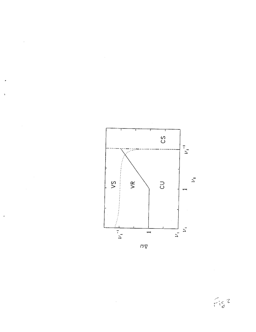
Figure 2: Schematic stability diagram for the convective growth rate. The solid line corresponds to the boundary of the domain VR where the pump wave incoherence reduces the convective growth rate, and the dotted line is the boundary of the domain VS where it completely stabilizes the parametric coupling. The rightmost verticle line divides the coherently stable (CS) from the coherently unstable (CU) domains. This diagram assumes $\nu_{2}>\nu_{1}$ corresponding to the ordering assumed in the main text.

In Fig. 2 we reproduce the stability diagram corresponding to the reduction of the convective instability growth rate induced by the pump wave incoherence. This diagram has to be understood as representing the effect of pump bandwidth $\Delta\omega_{0}$ as a function of $\nu_{2}$, for $\gamma_{0}$ and $\nu_{1}<\nu_{2}$ given. As explained in the introduction to this Section, the convective instability represents the early or transient time behavior of the parametric coupling.

The domain of applicability of the statistical theory corresponds to the inequalities

$$\Delta\omega_{0}>\gamma_{0},$$

$$\Delta\omega_{0}>{\rm Max}\left(\nu_{1},\nu_{2}\right)=\nu_{2},$$

that is to say,

$$\Delta\overline{\omega_{0}}>1,$$

$$\Delta\overline{\omega_{0}}>\overline{\nu}_{2}.$$

The domain corresponding to these inequalitites is referred to as ”VR” in Fig. 2, and stands for ”convective growth rate reduction;” the solid line presents the boundary between the coherent and incoherent domains. The threshold VI.5 for convective instabilities is approximately $\gamma_{0{\rm conv}}=\left(\Delta\omega_{0}\nu_{1}\right)^{1/2}$, so that the pump wave incoherence induces a complete stabilization of the convective growth rate in the domain referred to as ”VS” in Fig. 2,

$$\Delta\overline{\omega}_{0}>\overline{\nu}_{1}^{-1}$$

The boundary of the convectively stable region is the dotted line as obtained from Eq. VI.5. Lastly the parametric system is coherently stable in the domain $\overline{\nu}_{2}>\overline{\nu}_{1}^{-1}$ (corresponding to the usual coherent condition for stability $\gamma_{0}^{2}<\nu_{1}\nu_{2}$), the boundary of which is represented by the dashed-dot-dot line.

VI.4.2 Absolute Instability

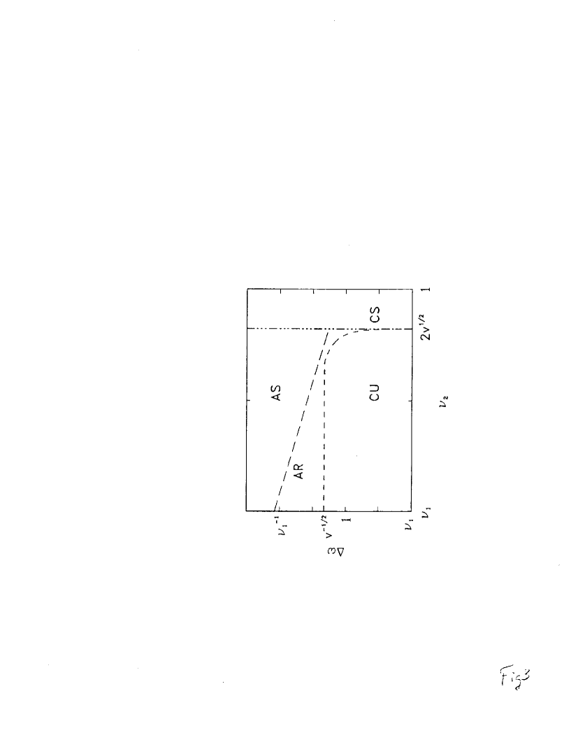
Figure 3: Schematic stability diagram for the absolute growth rate. The short-dashed line, between $\mid v\mid^{-1/2}$ on the vertical axis and $2\mid v\mid^{1/2}$ on the horizontal axis, represents the boundary of the domain AR where the pump wave incoherence reduces the absolute growth rate. Here $v=\mid v_{2}\mid$. The long-dashed line is the boundary of the domain AS where the pump wave incoherence completely stabilizes the absolute growth. To the right of the rightmost vertical line is the domain of coherent stability. This diagram assumes $\overline{\nu}_{2}>\overline{\nu}_{1}$.

In Fig. 3, we reproduce the stability diagram corresponding to the reduction of the absolute instability growth rate due to the pump incoherence, i.e. the growth reduction of the long time behavior of the parametric coupling in the case of existence of absolute instabilities. The domain of applicability of the statistical theory of absolute instabilities (VI.10) reads here $\Delta\omega_{0}>\gamma_{2}\mid V_{1}/V_{2}\mid^{1/2}$; on the other hand the threshold (VI.9b) is $\gamma_{0{\rm abs}}=\left(\Delta\omega_{0}\nu_{2}\right)^{1/2}$. The intersection between the two lines $\Delta\omega_{0}=\gamma_{0}\left(V_{1}/V_{2}\right)^{1/2}$ and $\Delta\omega_{0}=\gamma_{0}^{2}/\nu_{2}$ corresponds to $\nu_{2}=\gamma_{0}\left(V_{2}/V_{1}\right)^{1/2}$, which is smaller by a factor two than the usual coherent threshold for absolute instabilities, namely $\nu_{2}>2\gamma_{0}\left(V_{2}/V_{1}\right)^{1/2}$. Since the applicability condition for statistical theory has been obtained from strong inequalities (whereas the threshold condition $\gamma_{0{\rm abs}}=\left(\Delta\omega_{0}\nu_{2}\right)^{1/2}$ results from solving the RPA dispersion relation) the two limits could be reasonably made continuous between each other by writing the RPA validity condition as $\Delta\omega_{0}>\gamma_{0}\left(V_{1}/V_{2}\right)^{1/2}/2$ for $\nu_{2}<2\gamma_{0}\left(V_{2}/V_{1}\right)^{1/2}$. By doing so, the domain corresponding to a reduction of the absolute growth rate (henceforth referred to as the ”AR” domain) would be approximated by the inequality

$$\Delta\overline{\omega_{0}}>\left(2\mid v_{2}\mid^{1/2}\right)^{-1}$$

and the domain for complete stabilization of the absolute growth (referred to as the ”AS” domain) would be given by:

$$\Delta\overline{\omega_{0}}>\mid\overline{\nu}_{2}\mid^{-1}$$

Actually a more detailed calculation[46] based upon the exact dispersion relation (VI.15) shows that the AR domain corresponds to the inequality

$$\overline{\Delta\omega_{0}}>\mid v_{2}\mid^{-1/2}$$

for $\overline{\nu}_{2}<\mid v_{2}\mid^{1/2}$, and that the complete stabilization occurs when inequality (VI.23a) is satisfied in the range $\overline{\nu}_{2}<\mid v_{2}\mid^{1/2}$, and when the inequality

$$\Delta\overline{\omega}_{0}>2\mid v_{2}\mid^{-1/2}-\overline{\nu}_{2}\mid v_{2}\mid^{-1}$$

is fulfilled in the range $\mid v_{2}\mid^{-1}<\overline{\nu}_{2}<2\mid v_{2}\mid^{1/2}$.

In Fig. 3 the boundary of the AR domain is represented by a short-dashed line, and the boundary of the AS domain, computed from the incoherent threshold VI.9a, by a long-dashed line. One may see that the two boundaries almost coalesce at $\overline{\nu}_{2}=\mid v_{2}\mid^{1/2}$, $\Delta\omega_{0}=\mid V_{2}\mid^{-1/2}$; this simply means that the AR domain shrinks to zero in the limit $\mid v_{2}\mid\rightarrow 0$ for $\overline{\nu}_{2}>\mid v_{2}\mid^{1/2}$ (for this reason the short-dashed line, the long-dashed line, and the verticle dashed- dot-dot line bound a very small region for $\overline{\nu}_{2}>\mid v_{2}\mid^{1/2}$). The verticle line is the absolute coherent threshold Eq. VI.11b.

It can be easily checked that the domains corresponding to the approximate expression (VI.22a) and (VI.23a) do not significantly differ from the exact domains (VI.22b) and (VI.23b), in the range $\overline{\nu}_{2}<<\mid v_{2}\mid^{1/2}$, i.e. far from the absolute threshold. This result justifies in particular all the approximate expressions obtained in the remainder of our paper. On the other hand, in the range close to the absolute threshold, namely for $\mid v_{2}\mid^{1/2}<\overline{\nu}_{2}<2\mid v_{2}\mid^{1/2}$, this exact solution exhibits the additional AS domain $2\gamma_{0}\mid V_{1}/V_{2}\mid^{1/2}-\nu_{2}\mid V_{1}/V_{2}\mid<\Delta\omega_{0}<\gamma_{0}^{2}/\nu_{2}$, corresponding to a regime where a small $\Delta\omega_{0}$ may reduce the absolute growth rate. Such an effect is not really surprising since it means that a small frequency bandwidth may have a large effect when the parametric coupling is close to the coherent threshold, namely it converts an absolute instability into a convective one (which in turn gives rise to a spatial amplification, as it will be seen in VI.D3), by decreasing the usual coherent absolute threshold $\overline{\nu}_{2}=2\mid v_{2}\mid^{1/2}$ into the absolute threshold (VI.23b) modified by incoherency effects, namely $\overline{\nu}_{2}=2\mid v_{2}\mid^{1/2}-\mid v_{2}\mid\Delta\omega_{0}$.

VI.4.3 Spatial Amplification

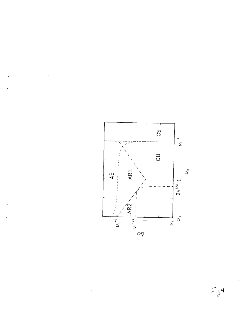
Figure 4: Schematic stability diagram for the spatial amplification growth rate. The dotted-dashed lines represent the boundaries of the domains AR1 and AR2 where the pump wave incoherence reduces the spatial amplification rate; the dotted line of crosses is the boundary of the domain AS (identical to the domain VS of Fig. 2) where it completely stabilizes spatial amplification. The short-dashed line (see Fig. 3) represents the threshold for the existence of absolute instabilities in the case $V_{1}V_{2}<0$. The rightmost vertical line separates the coherently stable (CS) and unstable (CU) domains. This diagram assumes $\overline{\nu}_{2}>\overline{\nu}_{1}$.

In Fig. 4, we reproduce the stability diagram corresponding to the reduction of the spatial amplification growth rate $\kappa^{sa}$. The first root (VI.13) for the spatial amplification growth rate is given in terms of dimensionless quantities as

$$\overline{\kappa}_{1}=-\left(\Delta\overline{\omega}_{0}\right)^{-1}$$

where the dimensionless growth rates $\overline{\kappa}$ are defined as $\overline{\kappa}=\kappa^{sa}V_{1}/\gamma_{0}$. The domain of existence of this root, referred to in Fig. 4 as ”AR1” (for ”spatial amplification reduction”), is defined by inequalities (VI.14) and (VI.15), namely

$$\overline{\Delta\omega}_{0}>1$$

$$\overline{\Delta\omega}_{0}>\overline{\nu}_{2}$$

$$\overline{\Delta\omega}_{0}>\overline{\nu}_{2}^{-1}$$

The boundary of this domain is represented by the dotted-dashed line in Fig. 4.

The threshold condition (VI.15) can be written as

$$\overline{\Delta\omega}_{0}<\overline{\nu}_{1}^{~{}-1}$$

The boundary of this domain ”AS” is given more exactly by the dotted line as in Fig. 2.

The spatial amplification growth rate for the second root is

$$\overline{\kappa}_{2}=-\left(\overline{\Delta\omega}_{0}v_{2}\right)^{-1}$$

and its domain of existence, referred to in Fig. 4 as ”AR2,” corresponds to the inequalities (VI.17) and (VI.18), i.e.

$$\Delta\omega_{0}<\overline{\nu}_{2}^{~{}-1}$$

$$\Delta\omega_{0}>\mid v_{2}\mid^{-1/2}$$

in addition to inequalities in (VI.25a) and (VI.25b). The boundary of this domain is represented by the decreasing dotted-dashed line and the dashed line in Fig. 4. It is interesting to remark that in the domain $\overline{\nu}_{2}>2\mid v_{2}\mid^{1/2}$, the coherent spatial amplification growth rate is $\overline{\kappa}_{coh}=-1/\overline{\nu}_{2}$ so that $\overline{\kappa}$ varies continuously from its coherent value to $\kappa_{1}=-1/\Delta\overline{\omega}_{0}$, along the boundary $\Delta\overline{\omega}_{0}=\overline{\nu}_{2}$ (the dotted-dashed line for $\overline{\nu}>1$), whereas $\overline{\kappa}$ is strongly reduced from $\overline{\kappa}_{\rm coh}$ to $\overline{\kappa}_{1}$ along the boundary $\overline{\Delta\omega}_{0}=1/\overline{\nu}_{2}$ (the dotted-dashed line for $\overline{\nu}_{2}<1$).

Similarly, in the domain $\overline{\nu}_{2}<<2\mid v_{2}\mid^{1/2}$, and $V_{1}V_{2}>0,\overline{\kappa}$ varies continuously from its coherent expression $\overline{\kappa}=-1/v_{2}^{1/2}$ to $\overline{\kappa}_{2}=-1/\Delta\overline{\omega}_{0}v_{2}$ along the boundary $\Delta\overline{\omega}_{0}=(V_{2})^{-1/2}$ between the coherent domain and the AR2 domain, whereas $\overline{\kappa}$ is strongly reduced from $\overline{\kappa}_{2}$ to $\overline{\kappa}_{1}$ along the boundary $\Delta\overline{\omega}_{0}=1/\overline{\nu}_{2}$ between the AR2 and AR1 domains.

Let us consider now the last case, corresponding to the domain $\overline{\nu}<<2\mid v_{2}\mid^{1/2}$ for $V_{1}V_{2}<0$. In this case there is no spatial amplification in the coherent regime, but an absolute instability characterized by a spatial growth rate $\overline{\kappa}^{abs}\sim-1/\mid v_{2}\mid^{1/2}$. We thus find the same continuity as the one observed in the previous case $V_{1}V_{2}>0$ along the boundary $\Delta\overline{\omega}_{0}=\mid v_{2}\mid^{1/2}$ between the spatial growth rate $\overline{\kappa}^{abs}$, corresponding to the coherent absolute instability, and the incoherent spatial amplification growth rate $\overline{\kappa}_{2}$; on the other hand $\overline{\kappa}$ is strongly reduced from $\overline{\kappa}_{2}$ to $\overline{\kappa}_{1}$ along the boundary between the AR2 and AR1 domains, as in the case $V_{1}V_{2}>0$. We may thus conclude that in all cases the boundary $\Delta\overline{\omega}_{0}=1/\overline{\nu}_{2}$, i.e. $\Delta\omega_{0}=\gamma_{0}^{2}/\nu_{2}$ in physical units, corresponds to a large reduction of the spatial amplification growth rate.

Lastly, we may give for the sake of completeness the expression of the space growth rate $\overline{\kappa}^{abs}$ associated with the incoherent absolute instability in the domain AR2. As stated before, for $V_{1}V_{2}<0$, the domain AR2 corresponds to a mixed situation where there is the coexistence of a spatial amplification characterized by $\overline{\kappa}_{2}=1/\Delta\overline{\omega}_{0}\mid v_{2}\mid$, (for $V_{1}>0$ and $V_{2}<0$) and of an absolute instability the space amplification growth rate of which is $\overline{\kappa}^{abs}=1/\Delta\overline{\omega}_{0}\mid v_{2}\mid^{1/2}$; one has thus $\mid\overline{\kappa}^{abs}\mid<<\mid\overline{\kappa}_{2}\mid$.

VI.4.4 Comparison of the Short Time and Long Time behaviors

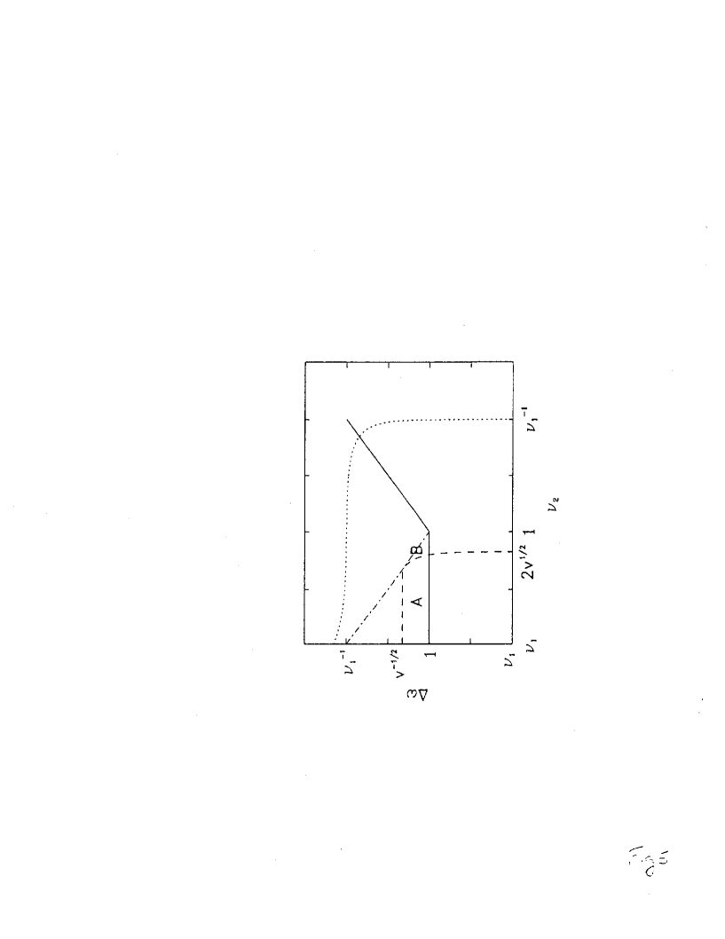
Figure 5: Comparison of the short time and long time behavior. The domains A and B correspond to regimes for which the pump wave incoherence reduces the initial parametric growth (convective growth) whereas the long time behavior remains unaffected. The meaning of the solid and dotted, the short-dashed, and the dotted-dashed lines are given in Figs. 2, 3, and 4 respectively. The diagram assumes $\overline{\nu}_{2}>\overline{\nu}_{1}$.

In Fig. 5 we reproduce the three boundaries found in the previous stability diagrams at which there is a reduction of the parametric growth due to the pump wave incoherence; the solid line corresponds to the boundary of the domain VR where the pump wave incoherence reduces the convective growth rate, i.e. where it modifies the short time behavior; the short- dashed line represents the boundary of the domain AR where the pump wave incoherence reduces the absolute growth rate, and the dotted-dashed line (which coincides with the solid line for $\overline{\nu}_{2}>1$) where it reduces the spatial amplification growth rate, i.e. the two domains where the long time behavior is modified. One immediately realizes that all the domains for which there is a growth reduction in the long time behavior are contained in the set for which there is a reduction of the initial growth, whereas the converse is not true. Thus the domain B in Fig. 5 is a domain where the spatial amplification is not affected by the pump wave incoherence although the convective growth is reduced in the initial stage; the same remark applies to the domain A for $V_{1}V_{2}>0$; for $V_{1}V_{2}<0$ this latter domain corresponds to a regime where the absolute instability growth rate, although much smaller than the convective growth rate, is not modified by the pump wave incoherence whereas the initial convective growth rate is reduced. We may have therefore the surprising conclusion that the reduction of the parametric growth is more difficult to achieve in the long time limit than in the initial stage.

VI.4.5 Finite Length Thresholds for Absolute Modes:

The thresholds set by the physical damping of the modes have been given for convective modes by (VI.5) and for absolute modes by (VI.9) in the incoherent limit or by (VI11b) in the coherent limit. In addition to satisfying these thresholds, the solutions must satisfy a threshold length criterion.

In the case of absolute instability, the length criterion in the coherent limit is known to be

$${\rm tan}\left({\gamma_{0}^{2}-\gamma_{abs}^{2}\over\mid V_{1}V_{2}\mid}\right)^{1/2}L=-\left({\gamma_{0}^{2}\over\gamma_{abs}^{2}}-1\right)^{1/2}$$

which in the absence of damping, $\gamma_{abs}$ sets

$$L={\pi\over 2}\sqrt{\mid V_{1}V_{2}\mid}\ \gamma_{0}.$$

A similar condition is obtained by solving the set (V.32) with $\nu_{j}=0$ and with the boundary condition $n_{1}(1)=n_{2}(L)=0$ for $V_{1}V_{2},0$ and $V_{1}<0$. This RPA threshold condition is given by the unusual expression,

$$L_{th}^{RPA}={\mid V_{1}V_{2}\mid\over 2\gamma_{0}^{2}}\left({\mid V_{1}\mid\over\Delta\omega_{2}}-{\mid V_{2}\mid\over\Delta\omega_{1}}\right)^{-1}{\rm ln}\left(\mid{V_{1}\over V_{2}}\mid{\Delta\omega_{1}\over\Delta\omega_{2}}\right),$$

which, not unexpectedly, does not reduce to the coherent expression as $\Delta\omega_{j}\rightarrow 0$. In the limit of purely temporal incoherence, (VI.30) reduces to

$$L_{th}^{RPA}={1\over 2}L_{g}^{2}{\Delta\omega\over V_{1}-V_{2}}{\rm ln}\mid{V_{1}\over V_{2}}\mid,$$

whereas, for purely spatial incoherence, (VI.30) reduces to

$$L_{th}^{RPA}={\Delta KL_{g}^{2}{\rm ln}\mid{V_{1}\over V_{2}}\mid\over\left(\mid{V_{1}\over V_{2}}\mid-\mid{V_{2}\over V_{1}}\mid\right)}.$$

The main point is that the ensemble averaged absolute growth rate for the infinite system given by VI.8a) in the RPA theory can be obtained only if the plasma size L sufficiently exceeds a length given by the maximum of (VI.29) and (VI.30).

VII Distribution of Mode Amplitudes and Intensities

The statistical analysis has obtained dispersion relations from which growth rates, thresholds, and amplification rates in different domains of incoherence were obtained for the ensemble averaged behavior of parametric instabilities with incoherent pump waves. In this analysis, some questions arose such as the validity of the RPA dispersion relation in the intermediate domain that can be answered in principle at least by a direct numerical integration of the coupled mode equations (II-10). Not only do we test the assumptions and approximations of the statistical analysis but, in Sec. VIIA, we illustrate the meaning of the averaging procedure. The fundamental assumption that the RPA equations apply in the whole incoherent domain is examined in Section (VII.B); finally the relation of the statistical growth rates and thresholds to the growth rates and thresholds of a particular model of induced laser beam incoherence is examined in Section (VII.C).

VII.1 Ensemble Average Growth Rates and the Distribution of Intensities

As has been noted at several points in this article, the incoherent absolute growth rates for the average intensity can be twice the rate expected on the basis of the growth rate for the average amplitude if certain inequalities are satisfied. For the purely temporal problem (where no distinction between absolute and convective is made), this factor of two arises if the damping is weak, specifically if Max $(\nu_{j})<\gamma_{0}^{2}/\Delta\omega_{0}$. However if this inequality is reversed, the average amplitude and average intensity growth rates are equal (we remind the reader that the definition of growth rates in Eq. III.9 removes the expected factor of two from the intensity growth rate). In the space-time problem considered in this article, one again notices a factor of two if $\mid V_{1}\mid=\mid V_{2}\mid$ in Eq. (VI.8a) for purely temporal incoherence, $\Delta\omega_{1}=\Delta\omega_{2}=\Delta\omega_{0}$. If one realizes that these random processes lead to a distribution of mode amplitudes f(a) after a time T, then it is clear that the first moment $\langle a\rangle=\int daf(a)$ and the second moment $\langle\mid a^{2}\mid\rangle=\int f(a)$ will be related only in special cases by $\langle\mid a^{2}\mid\rangle=\mid\langle a\rangle\mid^{2}$. If the distribution remains narrow then these two moments are simply related. However we will discover that, in some cases, that is just when there is this factor of two at issue, the distribution is broad. The second moment then depends on finding the distribution of rare events where the wave amplitude grows to larger amplitude than the mean amplitude. We anticipate the result that the width of the distribution increases in time as does the mean so that the task of computing the ensemble average $\langle\mid a^{2}\mid\rangle$ is increasingly more difficult as the sampling time is increased.

VII.1.1 Purely Temporal Evolution

These remarks are now illustrated by considering the coupled mode equations for the purely temporal problem which have the simple form given by

$$\left({\partial\over\partial t}+\nu_{1}\right)a_{1}(t)=\gamma_{0}\tilde{S}(t)a_{2}^{*}(t),$$

$$\left({\partial\over\partial t}+\nu_{2}\right)a_{2}(t)=\gamma_{0}\tilde{S}(t)a_{1}^{*}(t).$$

In previous work, an exact solution for the ensemble average mode amplitude and intensity was found when $\tilde{S}(t)$ is a Kubo-Anderson process (Section V.1). When $\Delta\omega_{0}>\gamma_{0}^{2}\ \Delta\omega_{0}>\nu_{1},\nu_{2}$ the growth rates are found to be $\gamma_{\langle a\rangle}$ and $\gamma_{\langle a^{2}\rangle}=2\gamma_{0}^{2}\ \Delta\omega_{0}$. Here, we are interested in the fluctuations of the amplitude and intensity about the means $\langle\mid a\mid\rangle$ and $\langle\mid a\mid^{2}\rangle$. Some useful insight can be gained into this question of fluctuations and its influence on the behaviors of $\mid a\mid$ and $\mid a\mid^{2}$ by considering the simplest possible model, that of two coupled undamped modes $a_{1}$ and $a_{2}$ described by Eqs. (VII.1) where $\tilde{S}(t)={\rm exp}(i\phi(t))$ and $\phi(t)$ is a random phase with bandwidth $\Delta\omega_{0}$. In this simple case we will be able to calculate the evolution of the distribution function f(a) of amplitudes.

Because $q=\mid a_{1}\mid^{2}-\mid a_{2}\mid^{2}$ is a constant of the motion, we can conveniently write:

$$a_{1}=q^{1/2}{\rm cosh}\theta e^{i\phi_{1}}$$

$$a_{2}=q^{1/2}{\rm sinh}\theta e^{i\phi_{2}}$$

from which the equations of motion (VII.1) imply

$${\partial\theta\over\partial t}=\gamma_{0}{\rm cos}\psi$$

$${\partial\psi\over\partial t}=-2\gamma_{0}\,{\rm coth}2\theta\,{\rm sin}\psi+{\partial\phi\over\partial t}$$

where

$$\psi\equiv\phi_{2}-\phi_{1}+\phi$$

If we define a distribution function $f(\theta,\psi,t)$, it evolves according to the Fokker-Planck equation:

$${\partial f\over\partial t}+{\partial\over\partial\theta}\gamma_{0}{\rm cos}\psi f-{\partial\over\partial\psi}2\gamma_{0}{\rm coth}2\theta\,{\rm sin}\psi f=\Delta\omega_{0}{\partial^{2}f\over\partial\psi^{2}}$$

In the large bandwidth limit $\Delta\omega_{0}>>\gamma_{0}$, $\partial/\partial t$., we can use a Chapman-Enskog like procedure, expanding $f=f_{0}+f_{1}+...$ and to zero order obtain $\partial^{2}f_{0}/\partial\psi^{2}=0$, so that $f_{0}=f_{0}(\theta,t)$ independent of $\psi$. To first order we obtain

$$f_{1}=-{\gamma_{0}\over\Delta\omega_{0}}{\rm cos}\psi\left({\partial f_{0}\over\partial\theta}-2{\rm coth}2\theta f_{0}\right)$$

and to second order

$${\partial f_{0}\over\partial t}-{\gamma_{0}^{2}\over\Delta\omega_{0}}{\rm cos}^{2}\psi{\partial\over\partial\theta}\left({\partial\over\partial\theta}-{\rm coth}2\theta\right)f_{0}-{\partial\over\partial\psi}2\gamma_{0}{\rm coth}2\theta\,{\rm sin}\psi f_{1}=\Delta\omega_{0}{\partial^{2}f_{2}\over\partial\psi^{2}}$$

Averaging over $\psi$, we obtain the consistency equation,

$${\partial f_{0}\over\partial t}={1\over 2}{\gamma_{0}^{2}\over\Delta\omega_{0}}{\partial\over\partial\theta}\left({\partial\over\partial\theta}-{\rm coth}2\theta\right)f_{0}$$

We are interested in the evolution of f from an initial condition $f(t=0)=\delta(\theta-\theta_{0})$. If we assume $\theta>>1$, since we expect $\theta$ to increase we can approximate ${\rm coth}2\theta=1$ in the above equation. It is then readily solved obtaining

$$f=\left(2\pi\gamma_{0}^{2}t/\Delta\omega_{0}\right){\rm exp}\left(-\left(\theta-\theta_{0}-\gamma_{0}^{2}t/\Delta\omega_{0}\right)^{2}/\left(2\gamma_{0}^{2}t/\Delta\omega_{0}\right)\right);$$

that is, $\theta$ is Gaussian distributed with mean $\theta_{0}+\gamma_{0}^{2}t/\Delta\omega_{0}$ and variance $\gamma_{0}^{2}t/\Delta\omega_{0}$. This distribution is shown in Fig. 7.1 for $\Delta\omega_{0}=10\gamma_{0}$ and $\gamma_{0}t=50$ together with some numerically generated distributions. Clearly then $\langle a^{-1}{\partial a\over\partial t}\rangle={\partial\over\partial t}\langle\theta\rangle=\gamma_{0}^{2}/\Delta\omega_{0}$ and $\langle a\rangle\simeq q^{1/2}{\rm exp}\left(\theta_{0}+\gamma_{0}^{2}t/\Delta\omega_{0}\right)$. On the other hand, if we calculate $\langle\mid a\mid^{n}\rangle\simeq q^{n/2}\langle{\rm exp}\left(n\theta\right)\rangle$, we obtain

$$\langle\mid a\mid^{n}\rangle\sim\mid a\mid_{0}^{n}{\rm exp}\left(n\left(n+2\right)\gamma_{0}^{2}t/2\Delta\omega_{0}\right).$$

For the special case n = 2 we observe that the growth rate for $\langle\mid a\mid^{2}\rangle$ is $4\gamma_{0}^{2}/\Delta\omega_{0}$, containing the factor of two noted earlier. In particular we see explicitly that the mean growth rate is definition dependent because the distribution of growth rates is so broad. To compare with these analytic results, Eqs. (VII.1) were numerically integrated for a large number of different independent realizations of a Kubo-Anderson process such that $\gamma_{\langle a\rangle}T>>1$ and $\Delta\omega_{0}=10\gamma_{0}$. In Fig. 6, the distribution (broken line) of the intensity $\mid a\mid^{2}$ is shown for $T\gamma_{0}=50$ and $2\times 10^{3}$ realizations. The ”measured” value of $\gamma_{\langle a\rangle}$ is 0.095 and $\gamma_{\langle a^{2}\rangle}$ is 0.16, and obviously the distribution at $\mid a\mid^{2}={\rm exp}\left(4\gamma_{0}^{2}T/\Delta\omega_{0}\right)={\rm exp}\left(20\right)=10^{8.7}$ is not resolved. Moreover, the few events with $\mid a\mid^{2}>10^{7.2}$ that have grown at the rate greater than 0.165 $\gamma_{0}$ have determined $\gamma_{\langle a^{2}\rangle}$. In general, the accurate numerical computation of random multiplicative processes in which rare events determine the quantity of interest is nontrivial[77]. On the other hand, the distribution of events that have grown at the rate $\gamma_{\langle a\rangle}$ is well resolved. When there is sufficient damping, i.e. Max $\left(\nu_{1},\nu_{2}\right)\geq\gamma_{0}^{2}/\Delta\omega_{0}$ the exact theoretical results show the ensemble average growth rate $\gamma_{\langle a^{2}\rangle}\simeq\gamma_{\langle a\rangle}$. The simulation results for $\nu_{2}=\gamma_{0}$ also shown in Fig. 6 (dashed-dotted line), demonstrate that the damping has dramatically narrowed the distribution of $\mid a\mid^{2}$ so that $\gamma_{\langle a^{2}\rangle}=0.092$ and $f(a^{2})$ is zero for $\mid a^{2}\mid>10^{5}$.

Note that this behavior is not specific to the Kubo-Anderson process. Numerical simulations with a randomly diffusing phase or a K-A process with equally spaced elapsed times obtained similar distributions of $\mid a^{2}\mid$.

VII.1.2 Space-time Evolution of Absolute Instabilities

Here, the incoherent absolute growth rate $\gamma_{\langle\mid a^{2}\mid\rangle}$ for temporal incoherence is twice the ”nominal” incoherent growth rate, $\gamma_{inc}\equiv\gamma_{0}^{2}/\Delta\omega$, if $\mid V_{1}\mid=\mid V_{2}\mid$. Given the results just presented for the purely temporal problem, this factor of two suggests that we might expect a broad distribution to result from considering different realizations of a temporal random process with bandwidth $\Delta\omega_{0}$. In this case, we remind the reader that no absolute instability is allowed by the average amplitude equations since the average amplitude equations decouple in the RPA or Bourret approximation. It is also interesting to observe that, unlike the purely temporal case, damping on either mode does not affect the factor that multiplies $\gamma_{inc}$ to obtain $\gamma_{\langle a^{2}\rangle}$. This factor, $q=1+2\sqrt{V_{1}V_{2}}/\left(\mid V_{1}\mid+\mid V_{2}\mid\right)$, depends on the ratio of the group velocities and approaches two when the group velocity ratio approaches one. Thus, in analogy with the purely temporal problem, we expect the distribution of intensities of growing modes to broaden as the group velocity ratio approaches one.

Before we proceed to test this hypothesis, we must be certain that both the incoherent absolute growth rate $\gamma_{\langle a^{2}\rangle}$ (VI.8a) is less than the coherent rate (VI.IIa) and that the plasma length exceed sufficiently the threshold lengths (VI.31) and (VI.29a). In addition the threshold set by the physical damping and bandwidth must be exceeded. These conditions are met by choosing the parameters: $\nu_{j}=0$, $j=1,2$, $\Delta\omega_{0}=10\gamma_{0}$, and $L=10L_{g}$. When the group velocity ratios $V_{1}/V_{2}=-16$ and -100, the predicted incoherent absolute growth rates $\gamma_{\langle\mid a^{2}\mid\rangle}$ are 0.147 and 0.12 $\gamma_{0}$, respectively. The predicted coherent absolute rates are 0.47 and 0.2 $\gamma_{0}$ respectively.

The distribution of $\mid a^{2}\mid$ for $\Delta\omega_{0}=10\gamma_{0}$ is shown in Fig. 7.2 for each velocity ratio. Each event in the distribution represents the ratio $a_{1}^{2}(T)=\mid a_{1}\left(X_{0},T\right)\mid^{2}/\mid a_{1}\left(X_{0},t_{0}\right)\mid^{2}$ where $\gamma_{0}\left(T-t_{0}\right)=45$ and $X_{0}$ is the initial position of a source at t = 0 in $a_{2}$. The time $t_{0}$ is chosen nonzero to avoid the influence of transients and was $20\gamma_{0}^{-1}$ in all these cases. This ”initial” time is longer than the time for the convective pulse to move across the system, $t_{c}=2L/\left(\mid V_{1}\mid+\mid V_{2}\mid\right)$ but not always longer than the time it takes the slow wave to transit the length L. However since the growth is measured at the source point, the fact that in the entire plasma, the waves are not growing at the asymptotic rate should not matter.

In these simulations, the numerically calculated ensemble average growth rate $\gamma_{\langle a^{2}\rangle}^{sim}$ was smaller than the RPA prediction in all cases as expected. When the velocity ratio $V_{1}/V_{2}=-16$ and -100 the computed $\gamma_{\langle a^{2}\rangle}^{sim}$ was 60% and 75% respectively of the RPA prediction. However, we were most interested n the width of the distribution. When $\mid V_{1}/V_{2}\mid$ was 16 and 100, the full width at half maximum of the distribution was 7% and 2% of the peak respectively, and thus displayed the narrowing expected. When $V_{1}/V_{2}=-1$, the computed distribution was not significantly broader than the distribution for $V_{1}/V_{2}=-16$. Thus the difference in growth rates between $V_{1}/V_{2}=-1$ and -16 may arise from differences in the unresolved tail of the distribution.

We conclude from this study that the RPA growth rates for the ensemble average intensity are correct but in a given simulation, or perhaps a particular experiment, the measured growth rate may well be a factor of two smaller. However when the group velocity is large, as is typically the case of physical interest, the RPA predictions are more representative of the typical behavior.

VII.2 The RPA Conjecture

The question here is whether the RPA equations are applicable in the whole domain defined by the inequalities $\Delta\omega_{1}>{\rm Max}\left(\gamma_{0},\nu_{1}\right)$ and $\Delta\omega_{2}>{\rm Max}\left(\gamma_{0},\nu_{2}\right)$ or whether there is an intermediate domain when one of the cross inequalities $\Delta\omega_{1}>\nu_{2}$ or $\Delta\omega_{2}>\nu_{1}$ is not satisfied. To examined this case we look at the spatial Kubo-Anderson (K-A) process analyzed previously²⁷ with zero temporal incoherence and spatial correlation function with the property

$$\langle S\left(x\right)S^{*}\left(x+\Delta x\right)\rangle_{x}={\rm exp}\left(-\Delta K\Delta x\right).$$

If we assume $\mid V_{1}\mid>>\mid V_{2}\mid$ and $V_{1}V_{2}<0$, then the intermediate domain is described by the chain of inequalities,

$$\Delta KV_{1}>\nu_{1}>\mid\Delta KV_{2}\mid>\nu_{2},\gamma_{0}.$$

A physical example that might produce this set of inequalities is two plasmon decay in the presence of stationary ion acoustic turbulence where the shorter wavelength Langmuir wave is more strongly damped and has a faster group velocity. The choices in our numerical solution were:

$${\Delta K\mid V_{1}V_{2}\mid^{1/2}/\gamma_{0}=4,\hskip 5.69046pt\nu_{1}=2\gamma_{0},\hskip 5.69046pt\nu_{2}=0,\hskip 5.69046ptV_{1}/V_{2}=-16,}$$

for which the RPA equation absolute instability growth rate $\gamma_{\langle a^{2}\rangle}=0.12\gamma_{0}$ and the absolute instability coherent growth rate (VI.11), $\gamma_{\rm coh}^{abs}=0.35\gamma_{0}$. The simulation region $L=8L_{g},\left(L_{g}=\mid V_{1}V_{2}\mid^{1/2}/\gamma_{0}\right)$ was larger than the threshold length given by the maximum of Eq. VI.32 and VI.29.The simulation was run until $\gamma_{0}t=50$ for 1000 independent realizations of this spatial K-A process. An initial value was given to the undamped wave at t = 0 but the intensity at $\gamma_{0}T=50$ was measured relative to the intensity at $\gamma_{0}t_{0}=20$ because by that time the modes were observed to grow at this time asymptotic rate. The ensemble averaged rate $\gamma_{\langle a^{2}\rangle}$ was found to be independent of whether its calculation was based on the intensity at the source point $\mid a_{1}\left(X_{0},T\right)\mid^{2}$ or the total mode ”energy” $\int dx\mid a_{1}\left(x,T\right)\mid^{2}$. The results support our conjecture that the RPA equations apply in the whole incoherent domain, because the measured intensity growth rate, $\gamma_{\langle a^{2}\rangle}^{sim}=0.11\gamma_{0}$ agreed with the RPA rate $\gamma_{\langle a^{2}\rangle}=0.12\gamma_{0}$. However, the distribution of intensity at $\gamma_{0}T=50$ (relative to $\gamma_{0}t_{0}=20$) displayed in Fig 8 showed that, in fully a third of the cases, no growth occurred and that the remaining distribution consisted of a slowly decreasing tail. The maximum intensity in the distribution was achieved by a mode that grew at close to the coherent rate. In addition, the faster growth rates were achieved in cases in which there was an abnormally long distance between phase changes; in the maximum growth case, this distance was 2.18 $L_{g}$. As we remarked at the outset of this section and in the introduction (Sec. I), the growth of parametric instabilities with this model of spatial incoherence was studied by Williams et al. using more sophisticated statistical methods (quite different in nature to those used in this article) with the result that the fastest growing mode grows at the rate $\gamma_{f}$, given by Eq. I-9. This rate $\gamma_{f}$ depends on the size of the system, which is understood on the basis that as the system gets larger there is an increasing possibility that there will be a large region with no phase change. In our simulation this size dependent factor ${\rm ln}\Delta KL=3.47$ turns out to be approximately equal to the numerical factor of 4 in the RPA growth rate (Eq. VI.8a); all other factors are identical and $\Delta K\rightarrow\Delta k_{0}$. Unfortunately it is not feasible to simulate a system that doubles the size of this logarithmic factor with a constant value of $\Delta K$. Thus these simulations do not distinguish between the RPA theory and the results of Williams et al. However, the simulations do support the conjecture that the incoherent results apply in whole incoherent domain.

VII.3 Modeling of Induced Spatial Incoherence

One motivation for this work is the induced spatial incoherence technique (ISI) for creating smoothed laser beam intensity distributions in the focal plane. In this technique, statistically independent beamlets overlap and thereby produce both intensity and phase variations. Only pumps with phase variation alone have been considered up to this point in our numerical examples. Here we wish to show that the same statistical methods are valid for intensity and phase varying pumps if the conditions for the incoherent results to apply are met.

A model that exhibits both intensity and phase variation in one dimension is given by,

$$S\left(x,t\right)={1\over\sqrt{N}}\sum^{N}_{j=1}{\rm exp}\left\{i\,\delta K_{j}x+i\phi_{j}\left(t\right)\right\},$$

when $\delta K_{j}$ is uniformly distributed on $(0,K_{m})$ and $\phi_{j}(t)$ is a random variable of time. Each $\phi_{i}$ varies independently with the same mean coherence time, $\left(\Delta\omega_{0}\right)^{-1}$. The spatial coherence length in this model, $x_{c}=\pi/K_{m}$, is related to the focal length of the focussing optic. A shorter focal length results in a shorter coherence length.

At any given point and instant of time, the intensity $\mid S\left(x,t\right)\mid^{2}$, being the absolute square of the sum of N complex numbers of length N^-1/2, is Gaussian distributed with unit mean and variance. Because the sum varies with position over a length scale $x_{c}$, the instantaneous spatial intensity pattern is quite spikey with peak to average variations of more than two quite common. However because the sum at a given spatial position also varies in time with coherence time $\left(\Delta\omega_{0}\right)^{-1}$, the time averaged intensity is a much smoother function of space. Clearly if $\phi_{j}\left(t\right)$ is constant in time, then the spikey intensity pattern of Eq. VII.15 is stationary which can lead in the coherent domain to growth enhanced relative to a uniform intensity. Even in the incoherent domain without temporal bandwidth, we saw in the previous section that there is a finite probability, especially in large systems, for the phase to remain constant for a large distance. With phase and intensity variations, large fluctuations in growth rates are expected in the absence of temporal bandwidth. In the complementary limit where $\Delta\omega_{1}\geq\Delta\omega_{2}>{\rm Max}\left(\gamma_{0},\nu_{1},\nu_{2}\right)$, the results of our statistical analysis should apply. For simplicity, we choose to compute the convective growth for both temporal and spatial incoherence in the incoherent limit and for large group velocity ratios, $\mid V_{1}/V_{2}\mid>>1$. With a single term in the sum in Eq. VII.15 and $\Delta\omega_{1}=\Delta\omega_{2}=\Delta\omega_{0}$, the convective growth rate was in agreement with Eq. (VI.7). With no temporal bandwidth, $\Delta\omega_{0}=0$, the pump intensity has striking amplitude variation with peak to average variations of more than three to one. Nonetheless if $\mid\Delta KV_{2}\mid>\overline{\gamma}_{0}$, the convective growth rate, is reduced according to Eq. (VI.7) even if $\Delta\omega_{0}=0$. As the spatial incoherence weakens and the boundary $\Delta KV_{2}=\overline{\gamma}_{0}$ is approached for $\Delta\omega_{0}=0$ the measured growth rate in the simulations diverges from Eq. (VI.7) until, for $\overline{\gamma}_{0}>\mid\Delta KV_{2}\mid$, growth rates in excess of $\overline{\gamma}_{0}$ can occur with large fluctuations from case to case. Laser bandwidth, even if $\Delta\omega_{0}<\overline{\gamma}_{0}$, reduces both the fluctuations and the growth rate to less than $\overline{\gamma}_{0}$. Thus, some bandwidth is needed in this model to provide a smooth transition from the coherent to incoherent domain. Other models such as the one used in Section VII.B have the property that $\mid S\left(x,t\right)\mid=1$ so that the statement that pump incoherence can only reduce the growth rate is indeed true. Simulations in that case do show a smooth transition from the coherent to incoherent growth rate

VIII Conclusions and Applications

A comprehensive treatment of the effects of pump wave temporal and spatial incoherence has been presented for a homogeneous plasma. Eschewing specific models of incoherence that allow exact solutions, we have derived equations for ensemble averaged mode intensity and amplitudes in the incoherent limit. At each step in the process of deriving these approximate statistical equations, the conditions that must be satisfied are clearly stated. Thus, the meaning of incoherence in the context of parametric instability theory is carefully defined. The set of inequalities that comprise this definition form a major contribution of this work. Of course, the primary contribution of this work is the set of thresholds, growth rates, and amplification rates for both coherent and incoherent, convectively and absolutely unstable parametric interactions.

However, the majority of our readers are interested in the more practical results concerning thresholds, growth rates, and amplification coefficients as they pertain to laser plasma interactions. In a subsequent work,⁶ we will apply the results presented here to particular instabilities, and include both backscatter and sidescatter geometries. Here, we briefly consider the examples of stimulated Raman and Brillouin backscatter for parameters of interest to laser fusion. We choose the electron temperature, $T_{e}=3{\rm keV}$, the charge state Z = 40, the atomic number A = 80, the laser wavelength, $\lambda_{0}=0.35\mu m$, the laser intensity I = 10¹⁵ W/cm² and the electron density, $N_{e}=0.2N_{c}$ for SRS and 0.25 N_c for SBS. Here N_c is the critical electron density defined by $4\pi N_{c}e^{2}/m_{e}=\omega_{0}^{2}$. For almost all calculations it is the ratio Z/A and not Z or A by themselves that is important.

The nominal SBS growth rate is $\gamma_{0}^{srs}=2.5\times 10^{-3}\omega_{0}$ whereas the SRS coherent convective threshold, Eq. (I-1) is $\gamma_{0}^{conv}=3.2\times 10^{-4}\omega_{0}$. Landau damping was neglected because for $T_{e}=3{\rm keV}$, an electron density can always be chosen to make it negligible. Thus SRS is an order of magnitude above threshold. The laser bandwidth sufficient to achieve convective stability can be found by using Eq. (VI.5). We find $\Delta\omega_{c}=4.5\times 10^{-2}\omega_{0}$. On the other hand, the coherent threshold for absolute instability given by Eq. (VI.9a), $\gamma_{0abs}=1.510^{-3}\omega_{0}$, is exceeded by less than a factor of two. However, as we have emphasized, in Sec. VI, relatively large laser bandwidth is required to reduce the absolute growth rate. Satisfying the validity conditions for using the incoherent formula, Eq. (VI.10), imposes the condition, $\Delta\omega_{0}/\omega_{0}=10^{-2}$, which is, coincidentally, the same condition numerically that is required for absolute stability as determined by Eq. (VI.9a).

The SBS thresholds are dependent on the ion acoustic damping rate and thus the ion temperature, $T_{i}$. However, even if $T_{i}=T_{e}$ the ion Landau damping is negligible for $Z>10$. Thus, the ion acoustic damping rate is determined by the electrons and is given by $\gamma_{ac}/\omega_{0}=2.3\times 10^{-5}$. Hence, the convective coherent threshold $\gamma_{0conv}/\omega_{0}=1.5\times 10^{-4}$ is easily exceeded by the nominal SBS growth rate $\gamma_{0}=7\times 10^{-4}\omega_{0}$. In addition, the SBS absolute instability coherent threshold $\gamma_{0abs}=3.4\times 10^{-4}\omega_{0}$ is exceeded. Here, the bandwidth required to achieve convective stability is $\Delta\omega_{c}/\omega_{0}=2.2\times 10^{-2}$. Moreover, the bandwidth required for absolute stability is by accidental choice of parameters, the same as for convective stability because although $\nu_{1}<<\nu_{2}$, nonetheless $\left(V_{1}/V_{2}\right)\nu_{2}>\nu_{1}$ and the incoherent absolute threshold Eq. (VI.9a) reduces to the incoherent convective threshold Eq. (VI.6). At this point, we should warn the reader that the results reported here assumed the validity of the coupled mode equations which requires the mode frequencies $w_{j}>\Delta\omega_{0}$ for j = 0,1,2. However, we have in the case of SBS a critical bandwidth for stability that exceeds the ion acoustic frequency $\omega_{a}=2\times 10^{-3}\omega_{0}$. At the very least, one might expect additional stability when $\Delta\omega_{0}>\omega_{a}$. For a partial answer to the effects that $\Delta\omega_{0}>\omega_{a}$ has, we considered SBS again for the purely temporal problem without using the assumption that $\omega_{a}>>\Delta\omega_{0}$. We start with the equations,

$$\left({\partial\over\partial t}+\nu_{1}-i\delta\omega\right)a_{1}=-i\gamma_{0}a_{2}^{*},$$

$$\left({\partial^{2}\over\partial t^{2}}+\omega_{a}^{2}\right)a_{2}=-2\gamma_{0}\omega_{a}a_{1}^{*},$$

where $\delta\omega\equiv\omega_{0}-\omega_{1}$, is the difference between the pump frequency and the scattered light frequency. Here a_1,2 are the mode amplitudes for the scattered light and ion acoustic waves respectively. Two different dispersion relations are obtained, as expected, by obtaining equations for the evolution of average amplitude $\langle a_{j}\rangle$. The ion acoustic mode $\langle a_{2}\rangle$ dispersion relation is not affected by magnitude of $\Delta\omega_{0}/\omega_{a}$ so that the growth rate,

$$\gamma_{\langle a_{2}\rangle}=-\nu_{2}+{\gamma_{0}^{2}\over\left(\nu_{1}+\Delta\omega_{0}\right)},$$

is a maximum when $\delta\omega=\omega_{a}$. On the other hand, the dispersion relation for $\langle a_{1}\rangle$ is modified so that the growth rate when $\Delta\omega_{0}>>\omega_{a},\nu_{2}$,

$$\gamma_{\langle a_{1}\rangle}=-\nu_{1}+{3\sqrt{3}\over 4}{\omega_{a}\gamma_{0}^{2}\over\Delta\omega_{0}^{2}},$$

shows a stronger reduction with bandwidth than $\gamma_{\langle a_{2}\rangle}$. Here the maximum growth rate for $\langle a_{1}\rangle$ occurs for a bandwidth dependent real frequency $\omega_{0}-\omega_{1}=\Delta\omega_{0}/\sqrt{3}$. Thus, the threshold for mode $\langle a_{1}\rangle$ is increased when $\Delta\omega_{0}>\omega_{a}$ by the ratio $\Delta\omega_{0}/\omega_{a}$. The actual threshold for the coupled set VIII.1 is,

$$\gamma_{0conv}^{2}={\rm Min}\left(\nu_{2}\left(\nu_{1}+\Delta\omega_{0}\right),\nu_{1}\left(\nu_{2}+\Delta\omega_{0}\right){\rm Max}\left(1,{\Delta\omega_{0}+\nu_{2}\over\omega_{a}}\right)\right).$$

This equation (VIII.4) is a generalization of Eq. (VI.6). In our example, the threshold is not increased when $\Delta\omega_{0}>\omega_{a}$.

In our example, chosen for its relevance to laser fusion, the critical bandwidth to reach convective or absolute stability has been found to be 2-5% of the laser frequency. Such a bandwidth is beyond the currently achievable with any ICF laser system. However, novel techniques are being pursued that are capable of achieving these bandwidths[6]. In addition, there is the question of whether the average laser intensity or the larger hotspot intensity should be used in evaluating the thresholds. The use of the larger intensity would make the bandwidth requirements infeasible. However, if bandwidth is combined with a beam smoothing scheme, use of the mean intensity may be correct. Recent calculations[66,67] have shown that, for at least one such scheme, ISI, the use of the average intensity is justified.

In addition to temporal bandwidth, there is also the effect of spatial incoherence produced by beam smoothing techniques that lead to a spread of wavevectors, $\Delta k_{0}$. In the examples of backscatter considered previously in this section for temporal bandwidth, spatial incoherence will have little effect because $\Delta k_{0**}/\Delta k_{0*}\sim f^{\#-1}$ where the f number of the focussing optic, f#, is typically large in ICF applications. Furthermore, the wavenumber spread will not increase the convective threshold because the effective bandwidth, $\mid\Delta k_{0}\cdot V_{g{\rm min}}\mid$, is in general small compared to $\nu_{1},\nu_{2}$, and $\gamma_{0}$. However absolute instabilities with significant wavevectors perpendicular to the laser propagation axis such as two plasmon decay may be influenced significantly by such a spread since there $\Delta k_{*}V_{g*{\rm max}}$ will be the effective bandwidth.

The work reported here is only a step in the application of a statistical theory to particular instabilities. Further progress may require modifications or extensions to our work in order to remove some of the limitations of our approximations. We look forward to new developments in the theory and even more to the stimulus of experimental data.

References

• K. Moncur, Applied Optics, 16, 1449 (1977).

• R. H. Lehmberg and S. P. Obenschain, Opt. Commun. 46, 27 (1983).

• Y. Kato, K. Mima, N. Miyanaaga, S. Arinaga, Y. Kitagawo, M. Nakatsuka, and C. Yamanaka, Phys. Rev. Lett., 53, 1057 (1984); Y. Kato and K. Mima, Applied Physics 329, 186 (1982).

• S. Skupsky, R. W. Short, T. Kessler, R. S. Craxton, S. Letzring, and T. M. Soures, J. Appl. Phys. 66, 3456 (1989).

• D. Veron, H. Ayral, C. Gouedard, D. Husson, J. Lauriou, O. Martin, B. Meyer, M. Rostaing, and C. Sauteret, Optics Communications, 65 (1988).

• D. M. Pennington, M. A. Henesian, R. B. Wilcox, T. L. Wieland, D. Eimerl And H.T. Powell, “A Novel Bandwidth Source for Laser Experiments”, Technical Digest Series, Vol 18, CLEO ’94 Anaheim, Ca.

• D. Pesme, “Effects of Temporal and Induced Spatial Incoherence of Parametric Instabilities in Laser Plasma Interactions”, 1987 Annual Technical Report CNRS-LULI, Ecole Polytechnique. (available from NTIS, Springfield VA 22161: document PB 92-100312.)

• K. Nishikawa, in “Advances in Plasma Physics, Vol 6”, edited by A. Simon and W. B. Thompson (Wiley N. Y. 1976)

• G. M. Zaslavskii, V. S. Zakharov, Sov. Phys. Tech.  Phys.,

  12, 7 (1967).

• G. E. Vekshtein, G. M. Zablavskii, Sov. Phys. Doklady, 12, 34 (1967).

• E. J. Valeo and C. R. Oberman, Phys. Rev. Lett. 30, 1035 (1973).

• S. Tamor, Phys. Fluids 16, 1169 (1973).

• J. J. Thomson, W. L. Kruer, S. E. Bodner, and J. S. DeGroot, Phys. Fluids, 17, 849 (1974).

• J. J. Thomson and J. I. Karush, Phys. Fluids 17, 1608 (1974).

• J. J. Thomson, Nuclear Fusion, 15, 237 (1975).

• G. Laval, R. Pellat, D. Pesme, A. Ramani, M. N. Rosenbluth, and E. A. Williams, Phys. Fluids, 20, 2049 (1977).

• J. J. Thomson, Phys. Fluids, 21, 2082 (1978).

• W. L. Kruer, K. G. Estabrook, and K. H. Sinz., Nucl. Fusion, 13, 952 (1973).

• W. Kruer, E. Valeo, K. Estabrook, J. Thomson, B. Langdon, and B. Lasinski, Plasma Physics and Controlled Nuclear Fusion Research, Vol. II, 525 (1974).

• K. Estabrook, J. Harte, E. M. Campbell, F. Ze, D. W. Phillion, M. D. Rosen, and J. T. Larsen, Phys. Rev. Lett. 46, 724 (1981).

• D. W. Forslund, J. M. Kindel and E. M. Lindman, Phys Fluids, 18, 1017 (1975).

• K. Estabrook, W. L. Kruer, and B. F. Lasinski, Phys. Rev. Lett., 45, 1399 (1980).

• K. Estabrook and W. L. Kruer, Phys. Fluids, 26, 1892

• G. Bonnaud and C. Reisse, Nuclear Fusion, 26, 633 (1986).

• C. Yamanaka, T. Yamanaka, T. Sasaki, and J. Mizui, Phys. Rev. Lett., 32, 1038 (1974).

• R. R. Johnson, P. M. Campbell, L. V. Powers, and D. C. Slater, in proceedings of the Topical Meeting of Inertial Confinement Fusion, 7-9 February, 1978, San Diego (unpublished); D. C. Slater and D. J. Tanner, Proceedings of the Ninth Annual Conference on the Anomalous Absorption of Electromagnetic Waves.

• C. E. Clayton, C. Joshi, A. Yasuda and F. F. Chen, Phys. Fluids, 24, 2312 (1981).

• A. Mase, N. C. Luhmann, J. Holt, H. Huey, M. Rhodes, W. F. DiVergilio, J. J. Thomson, and C. F. Randall, Plasma Physics and Controlled Nuclear Fusion Research (IAEA, Vienna, 1981).

• R. Giles, R. Fedosejevs, and A. A. Offenberger, Physical Review A, 26, 1113 (1982).

• D. G. Colombant, W. M. Manheimer, and J. H. Gardner, Phys. Fluids 26, 3148 (1983).

• V. V. Tamoikin and S. M. Fainstein, Sov. Phys. JETP, 35, 115 (1972).

• S. A. Akhmanov, Yu. E. Dyakov and L. I. Pavlov, Sov. Phys. JETP, 39, 249 (1974).

• P. Kaw, R. White, D. Pesme, M. Rosenbluth, G. Laval, R. Varma, and R. Huff, Comments Plasma Phys. Controlled Fusion 2, 11 (1974).

• D. R. Nicholson and A. N. Kaufman, Phys. Rev. Lett., 33, 1207 (1974).

• M. Y. Yu, P. K. Shukla and K. H. Spatschek, Phys. Rev A, 12, 656 (1975)

• K. H. Spatschek, P. K. Shukla and M. Y. Yu, Phys. Lett. A, 51, 183 (1975).

• D. R. Nicholson, Phys. Fluids, 19, 889 (1976).

• G. Laval, R. Pellat and D. Pesme, Phys. Rev. Lett., 36, 192 (1976).

• E. A. Williams, J. R. Albritton, and M. N. Rosenbuth, Phys. Fluids 22, 139 (1979).

• E. Z. Gusakov and A. D. Piliya, Sov. J. Plasma Phys., 6, 277 (1980).

• E. Z. Gusakov and A. D. Piliya, Sov. J. Plasma Phys., 7, 733 (1981).

• E. Z. Gusakov and A. D. Piliya, Sov. J. Plasma Phys., 8, 324 (1982).

• W. Rozmus, A. A. Offenberger and R. Fedosejevs, Phys. Fluids, 26, 1071 (1983).

• A. Bourdier and E. A. Williams, ”Effects of Induced Spatial Incoherence on Raman Scattering,” Laser Program Annual Report 1986, Lawrence Livermore National Laboratory, UCRL-50021-86 (1986).

• E. A. Williams, R. L. Berger, and A. Bourdier, Laser Program Annual Report 1987, Lawrence Livermore National Laboratory, UCRL-50021-87 (1988), p. 2-48.

• A. Bortuzzo-Lesne, G. Laval, D. Pesme, and M. Casanova, ”Coefficient de retrodiffusion Brillouin stimulee lorsque l’onde laser est incoherente,” Annual Internal Report GILM, Ecole Polytechnique (1984).

• L. Lu, Phys. Fluids, 31, 3362 (1988).

• L. Lu, Phys. Fluids, B1, 1605 (1989).

• P. N. Guzdar, Phys. Fluids, B3, 2882 (1991).

• M. N. Rosenbluth, Phys. Rev. Lett. 29, 565 (1972).

• S. P. Obenschain, J. Grun, M. J. Herbst, K. J. Kearney, C. K. Manka, E. A. McLean, A. N. Mostovych, J. A. Stamper, R. R. Whitlock, S. E. Bodner, J. H. Gardner, and R.Lehmberg, Phys. Rev. Lett. 56, 2807 (1986).

• A. N. Mostovych, S. P. Obenschain, J. H. Gardner, J. Grun, K. J. Kearney, C. K. Manka,, E. A. McLean, and C. J. Pawley, Phys. Rev. Lett., 59, 1193 (1987).

• S. P. Obenschain, C. J. Pawley, A. N. Mostovych, J. A. Stamper, J. H. Gardner, A. J. Schmitt, and S. E. Bodner, Phys. Rev. Lett. 62, 768 (1989).

• O. Willi, D. Bassett, A. Giulettii and S. J. Kartunnen, Opt. Comm., 70, 487 (1989).

• S. Coe, T. Afshar-rad, M. Desselberger, F. Khattak, O. Willi, A. Giulietti, Z. Q. Lin, W. Yu, and C. Danson, Europhys. Lett., 10, 31 (1989).

• S. E. Coe, T. Afshar-rad and O. Willi, Europhys. Lett., 13, 251 (1990).

• O. Willi, T. Afshar-rad, S. E. Coe and A. Guilettii, Phys. Fluids, B2, 1318 (1990).

• T. Afshar-rad, L. A. Gizzi, M. Desselberger, F. Khattak and O. Willi, Phys. Rev. Lett., 68, 942 (1992).

• T. Afshar-rad, S. E. Coe, O. Willi and M. Desselberger, Phys. Fluids, B4, 1301 (1992).

• W. Seka, R. E. Bahr, R. W. Short, A. Simon, R. S. Craxton, D. S. Montgomery and A. E. Rubenchik Phys. Fluids, B4, 2232 (1992).

• C. Labaune, S. Baton, T. Jalinaud, H. A. Baldis and D. Pesme Phys. Fluids, B4, 2224 (1992).

• J. D. Moody, H. A. Baldis, D. Montgomery, K. G. Estabrook, S. Dixit and C. Labaune, J. of Fusion Energy, 12, 323 (1993).

• T. Jalinaud, S. D. Baton, C. Labaune and H. A. Baldis, “Effets de lames de phases aleatoire sur les diffusions Brillouin et Raman stimulèes en plasma preforme”, LULI 1992 Annual Report, p56.

• C. Labaune, S. D. Baton, T. Jalinaud, E. Schifano, N. Renard, D. Pesme, H. A. Baldis, J. D. Moody and K. Estabrook, “Effet du lissage optique par lame de phase aleatiore sur les instabilities parametriques”, LULI 1992 Annual Report, p23.

• J. D. Moody, H. A. Baldis, D. S. Montgomery, K. Estabrook, R. L. Berger, E. A. Williams, W. L. Kruer and S. Dixit (submitted to Phys. Plasmas (1995)).

• R. L. Berger, Phys. Rev. Lett., 65, 1207 (1990).

• P. N. Guzdar, Phys. Fluids, B3, 776 (1991).

• H. A. Rose, D. F. Dubois and D. Russell, Sov. J. of Plasma Physics, 16, 537 (1990).

• A. Brissaud and U. Frisch, J. Math Phys., 15, 524 (1974); P. Kubo, ibid., 4, 174 (1963).

• R. Bourret, Nuovo Cimento, 26, 1 (1962).

• R. Z. Sagdeev and A. A. Galeev, Nonlinear Plasma Theory (Benjamin, New York, 1969).

• B. B. Kadomtsev, Plasma Turbulence (Academic Press, New York, 1965).

• V. N. Tsytovitch, Nonlinear Effects in Plasma (Plenum, New York, 1970).

• R. C. Davidson, Methods in Nonlinear Plasma Theory (Academic Press, New York, 1972).

• A. Bers and R. J. Briggs, Quarterly Progress Report No. 71, Research Laboratory of Electronics, MIT, p. 122,(1963) unpublished).

• V. P. Silin, Zh. Eksp. Teor. Fiz., 48, 1679 (1965) [Sov. Phys. JETP, 21, 1127 (1965)]; V. E. Zakharov, op. cit. 62, 1745 (1972) [op. cit. 35, 908 (1972)].

• S. Redner, Am. J. Phys. 58, 267 (1990).

Contents

1. I Introduction
2. II The Coupled Mode Equations
   1. II.1 The Coupled Mode Equations in Fourier Space.
   2. II.2 The Envelope Approximation for the Coupled Mode Equations in Real Space
3. III Statistical Description for Coupled Mode Equations
   1. III.1 The Frequency Mismatches
   2. III.2 The Incoherent and RPA domains
4. IV The Bourret Approximation for the Average Amplitudes
   1. IV.1 Introduction to the Bourret Approximation
   2. IV.2 The Bourret approximation for the average amplitude $<a_{i}>$
      1. IV.2.1 General three dimensional result.
      2. IV.2.2 Markov limit
   3. IV.3 The Special Case of a Kubo-Anderson Process
5. V The RPA Equations for the Wave Intensities
   1. V.1 The Bourret approximation in the limit $V_{g0}=\infty$.
   2. V.2 The RPA equations
6. VI Thresholds and Growth Rates for the Convective and the Absolute Instabilities and Spatial Amplification
   1. VI.1 Convective instabilities.
      1. VI.1.1 Domain of applicability of the RPA equations.
      2. VI.1.2 Convective instabilities expressions
   2. VI.2 Absolute instabilities
   3. VI.3 Spatial Amplification
   4. VI.4 Comparison of Stability Domains in the Case $V_{g0}=\infty$
      1. VI.4.1 Convective Instability
      2. VI.4.2 Absolute Instability
      3. VI.4.3 Spatial Amplification
      4. VI.4.4 Comparison of the Short Time and Long Time behaviors
      5. VI.4.5 Finite Length Thresholds for Absolute Modes:
7. VII Distribution of Mode Amplitudes and Intensities
   1. VII.1 Ensemble Average Growth Rates and the Distribution of Intensities
      1. VII.1.1 Purely Temporal Evolution
      2. VII.1.2 Space-time Evolution of Absolute Instabilities
   2. VII.2 The RPA Conjecture
   3. VII.3 Modeling of Induced Spatial Incoherence
8. VIII Conclusions and Applications