Quantum phases of mixtures of atoms and molecules on optical lattices

Abstract

We investigate the phase diagram of a two-species Bose-Hubbard model including a conversion term, by which two particles from the first species can be converted into one particle of the second species, and vice-versa. The model can be related to ultracold atom experiments in which a Feshbach resonance produces long-lived bound states viewed as diatomic molecules. The model is solved exactly by means of Quantum Monte Carlo simulations. We show that an ”inversion of population” occurs, depending on the parameters, where the second species becomes more numerous than the first species. The model also exhibits an exotic incompressible ”Super-Mott” phase where the particles from both species can flow with signs of superfluidity, but without global supercurrent. We present two phase diagrams, one in the (chemical potential, conversion)-plane, the other in the (chemical potential, detuning)-plane.

I Introduction

In the past years the Bose-Hubbard model Fisher89 has been extensively investigated and a lot of interest has been generated thanks to ultracold atom experiments on optical lattices Jaksch98 , which provide an ideal realization of the model. Recently, much theoretical and experimental work has been performed on mixtures with several species of particles. For instance, Bose-Fermi mixtures on lattices have been studied Ott04 ; Gunter06 ; Ospelkaus06 ; Pollet06 ; Sengupta07 ; Hebert06 . Another mixture that is likely of interest involves atoms and molecules, in which conversion between the two species is possible. Such conversion processes can describe, for instance, long-lived bound states of atoms (diatomic molecules) occuring in ultracold atom experiments where a Feshbach resonance is used to tune the scattering length of the atoms Timmermans ; Dickerscheid . In those experiments, the hyperfine interaction between two spin polarized atoms can flip the spin of one of the atoms, reducing sensitively their scattering length. The two atoms are virtualy bound into a ”molecular” state until the hyperfine interaction flips again the spin of one of the atoms.

II The model

With the motivation above, we propose to study a two-boson species model with an additional conversion term allowing two particles from the first species to turn into one particle of the second species, and vice-versa. We denote the first species as ”atoms”, and the second species as (diatomic) ”molecules”. Atoms and molecules can hop onto neighboring sites, interact, and conversion between two atoms and a molecule can occur. Several atoms can reside on the same site, their interaction being described by an on-site repulsion potential. A second on-site repulsion potential describes the interactions between molecules and atoms being on the same site. This leads us to consider the following Hamiltonian

$$\hat{H}=\hat{T}+\hat{P}+\hat{C},$$ (1)

with

$$\!\!\!\!\!\!\hat{T}\!=\!-t_{a}\!\!\sum_{\big{\langle}i,j\big{\rangle}}\!\!\big{(}a_{i}^{\dagger}a_{j}^{\phantom{\dagger}}+h.c.\big{)}-t_{m}\!\!\sum_{\big{\langle}i,j\big{\rangle}}\!\!\big{(}m_{i}^{\dagger}m_{j}^{\phantom{\dagger}}+h.c.\big{)}$$ (2)

$$\!\!\!\!\!\!\hat{P}\!=\!U_{aa}\!\sum_{i}\!\hat{n}_{i}^{a}\big{(}\hat{n}_{i}^{a}\!\!-\!\!1\big{)}\!+\!U_{am}\!\sum_{i}\!\hat{n}_{i}^{a}\hat{n}_{i}^{m}\!+\!D\!\sum_{i}\!\hat{n}_{i}^{m}$$ (3)

$$\!\!\!\!\!\!\hat{C}\!=\!g\sum_{i}\big{(}m_{i}^{\dagger}a_{i}^{\phantom{\dagger}}a_{i}^{\phantom{\dagger}}+a_{i}^{\dagger}a_{i}^{\dagger}m_{i}^{\phantom{\dagger}}\big{)}.$$ (4)

The $\hat{T}$, $\hat{P}$, and $\hat{C}$ operators correspond respectively to the kinetic, potential, and conversion energies. The $a_{i}^{\dagger}$ and $a_{i}^{\phantom{\dagger}}$ operators ($m_{i}^{\dagger}$ and $m_{i}^{\phantom{\dagger}}$) are the creation and annihilation operators of atoms (molecules) on site $i$, and $\hat{n}_{i}^{a}=a_{i}^{\dagger}a_{i}^{\phantom{\dagger}}$ ($\hat{n}_{i}^{m}=m_{i}^{\dagger}m_{i}^{\phantom{\dagger}})$ counts the number of atoms (molecules) on site $i$. Those operators satisfy the usual bosonic commutation rules $\big{[}a_{i}^{\phantom{\dagger}},a_{j}^{\dagger}\big{]}=\delta_{ij}$ and $\big{[}m_{i}^{\phantom{\dagger}},m_{j}^{\dagger}\big{]}=\delta_{ij}$. In order to simplify the model and reduce the space of parameters, we impose a hard-core constraint on molecules. This is done by adding the condition $m_{i}^{\phantom{\dagger}}m_{i}^{\phantom{\dagger}}=m_{i}^{\dagger}m_{i}^{\dagger}=0$. For a minimal model, we set a maximum of two atoms per site by imposing $a_{i}^{\phantom{\dagger}}a_{i}^{\phantom{\dagger}}a_{i}^{\phantom{\dagger}}=a_{i}^{\dagger}a_{i}^{\dagger}a_{i}^{\dagger}=0$. The sums $\big{\langle}i,j\big{\rangle}$ run over pairs of nearest-neighboring sites $i$ and $j$. We restrict our study to one dimension and we choose the atomic hopping parameter $t_{a}=1$ in order to set the energy scale, while we choose the molecular hopping parameter $t_{m}=1/2$, motivated by the continuous-space behavior of the hopping as a function of the mass ($t\propto\hbar^{2}/2m$), a molecule being twice heavier than an atom. Smaller values of $t_{m}$ (as mapping of experimental systems to Bose-Hubbard models would suggest Timmermans ; Dickerscheid ) are not expected to lead to qualitatively different behavior. The parameter $U_{aa}$ controls the interaction strength between atoms, and $U_{am}$ controls the interaction between atoms and molecules. The conversion between atoms and molecules is controlled by the positive parameter $g$. This parameter can be related to the ”hyperfine interaction” parameter in the Feshbach resonance picture Timmermans ; Dickerscheid . Finally, the parameter $D$ acts as a chemical potential for molecules, and allows to tune the energy difference between atomic and molecular states. This parameter can be related to the ”detuning” in the Feshbach resonance example. In the remainder of the paper we will not expand on the connection to the Feshbach resonance problem, nor attempt to reproduce Feshbach resonance physics. We concentrate on taking the model given in (1)–(4) at face value and determining its phase diagram. A similar model for the one-dimensional continuum has been analysed in Ref Gurarie , and for optical lattices in the mean field approximation Dupuis .

It is important to note that the Hamitonian (1) does not conserve the number of atoms $N_{a}=\sum_{i}a_{i}^{\dagger}a_{i}^{\phantom{\dagger}}$, nor the number of molecules $N_{m}=\sum_{i}m_{i}^{\dagger}m_{i}^{\phantom{\dagger}}$, because of the conversion term (4). However we consider that a molecule is made of two particles, so the total number of particles $N$ in the system is conserved:

$$N=N_{a}+2N_{m}.$$ (5)

III Quantum Monte Carlo simulations: The World Line algorithm

In order to make the model suitable for simulations, we perform a mapping of the Hamiltonian describing two species of bosons on a 1D lattice (1) onto a Hamiltonian describing single species of bosons evolving on a ladder (Fig. 1). In the 1D space, the two species live together. They can hop onto neighboring sites, and the interaction between the two species is described by an on-site potential $U_{am}$. The conversion between the two species occurs on a single site. In the ladder space, the atoms (molecules) live on the top (bottom) side of the ladder. The interaction between the two species is described by a potential $U_{am}$ acting between vertical neighboring sites. Two atoms living on the same atomic site can be destroyed at the same time, with the creation of a molecule on the corresponding molecular site (and vice-versa).

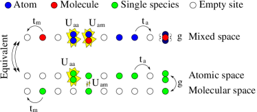
Figure 1: (Color online) In order to make the model suitable for simulations, a mapping is performed between the model of atoms and molecules living on a 1D lattice, and a model of single species where the particles reside on a ladder.

Quantum Monte Carlo simulations are performed for the ladder model by making use of the World Line algorithm Batrouni1990 ; Batrouni1992 . It is essential to emphasize that this algorithm works in the canonical ensemble, meaning here that the total number of particles $N=N_{a}+2N_{m}$ is conserved. Indeed, simulations using a grand canonical algorithm (Stochastic Series Expansion) Sandvik turned out to be difficult to handle, because it is numerically very hard to control the number of particles of each species using two chemical potentials, the number of particles of each species depending on both chemical potentials.

Defining the continuous product of evolution operators in imaginary time,

$$\prod_{0\to\beta}^{d\tau}e^{-d\tau\hat{H}}\hat{=}\lim_{M\to\infty}\prod_{k=1}^{M}e^{-\frac{\beta}{M}\hat{H}}=e^{-\beta\hat{H}},$$ (6)

one starts by writing the partition function as the trace of the evolution operator $e^{-\beta\hat{H}}$

$$\mathcal{Z}=\sum_{\psi}\left\langle\psi\right|\prod_{0\to\beta}^{d\tau}e^{-d\tau\hat{H}}\left|\psi\right\rangle$$ (7)

using the occupation number representation for the states $\left|\psi\right\rangle$. Then we use the so-called ”checkerboard decomposition” for the Hamiltonian, $\hat{H}=\hat{H}_{e}+\hat{H}_{o}$, with

$$\hat{H}_{e}=\sum_{i\,even}\hat{H}_{i}\hskip 56.9055pt\hat{H}_{o}=\sum_{i\,odd}\hat{H}_{i},$$ (8)

where $\hat{H}_{i}=\hat{T}_{i}+\frac{1}{2}\hat{P}_{i}+\frac{1}{2}\hat{C}_{i}$ and $\hat{T}_{i},\hat{P}_{i},\hat{C}_{i}$ are defined by

$$\hat{T}_{i} = -t_{a}\big{(}a_{i}^{\dagger}a_{i+1}^{\phantom{\dagger}}+h.c.\big{)}-t_{m}\big{(}m_{i}^{\dagger}m_{i+1}^{\phantom{\dagger}}+h.c.\big{)}$$ (9)

$$\hat{P}_{i} = U_{aa}\big{[}\hat{n}_{i}^{a}\big{(}\hat{n}_{i}^{a}-1\big{)}+\hat{n}_{i+1}^{a}\big{(}\hat{n}_{i+1}^{a}-1\big{)}\big{]}$$

$$+ U_{am}\big{(}\hat{n}_{i}^{a}\hat{n}_{i}^{m}+\hat{n}_{i+1}^{a}\hat{n}_{i+1}^{m}\big{)}$$

$$+ D\big{(}\hat{n}_{i}^{m}+\hat{n}_{i+1}^{m}\big{)}$$

$$\hat{C}_{i} = -g\big{(}m_{i}^{\dagger}a_{i}^{\phantom{\dagger}}a_{i}^{\phantom{\dagger}}+a_{i}^{\dagger}a_{i}^{\dagger}m_{i}^{\phantom{\dagger}}\big{)}$$

$$- g\big{(}m_{i+1}^{\dagger}a_{i+1}^{\phantom{\dagger}}a_{i+1}^{\phantom{\dagger}}+a_{i+1}^{\dagger}a_{i+1}^{\dagger}m_{i+1}^{\phantom{\dagger}}\big{)}.$$

We attract here the attention of the reader to Eq.III, in which we have added a minus sign to the conversion term. The energy of the model is independent of the sign in (III), so (III) and (4) are equivalent. This can be seen by realizing that flipping the sign of the conversion term just results in a redefinition of the phase of the molecular creation and annihilation operators, $m_{i}^{\dagger\prime}=-m_{i}^{\dagger}$ and $m_{i}^{\prime}=-m_{i}$. We work with a minus sign in (III) in order to ensure that all matrix elements $\big{\langle}\phi\big{|}e^{-\tau\hat{\mathcal{H}}}\big{|}\psi\big{\rangle}$ are positive. Those positive matrix elements normalized by $\mathcal{Z}$ define the probability of transition from the state $\big{|}\psi\big{\rangle}$ to the state $\big{|}\phi\big{\rangle}$, which is required for a Monte Carlo sampling.

It is important to note that $\hat{H}_{e}$ and $\hat{H}_{o}$ are written each as a sum of operators $\hat{H}_{i}$ that commute (but $\hat{H}_{e}$ and $\hat{H}_{o}$ do not commute). Using the Trotter-Suzuki formula at second order,

$$e^{-d\tau\big{(}\hat{H}_{e}+\hat{H}_{o}\big{)}}=e^{-\frac{1}{2}d\tau\hat{H}_{o}}e^{-d\tau\hat{H}_{e}}e^{-\frac{1}{2}d\tau\hat{H}_{o}}+\mathcal{O}(d\tau^{3}),$$ (12)

and using properties of the trace we get

$$\mathcal{Z}=\sum_{\psi}\left\langle\psi\right|\prod_{0\to\beta}^{d\tau}e^{-d\tau\hat{H}_{e}}e^{-d\tau\hat{H}_{o}}\left|\psi\right\rangle.$$ (13)

The error due to the Trotter-Suzuki decomposition vanishes because of the continuous product making $d\tau$ going to zero (in the case of a discrete product the Trotter error becomes $\mathcal{O}\big{(}d\tau^{2}\big{)}$ instead of $\mathcal{O}\big{(}d\tau^{3}\big{)}$, due to the accumulation of errors in the product). Introducing complete sets of states $I=\sum_{\psi(\tau)}\left|\psi(\tau)\right\rangle\left\langle\psi(\tau)\right|$ between each pair of exponentials leads to

$$\!\!\!\mathcal{Z}=\!\!\!\sum_{[\psi(\tau)]_{0}^{\beta}}\prod_{0\to\beta}^{d\tau}\left\langle\psi(\tau\!\!+\!\!d\tau)\right|e^{-d\tau\hat{H}_{e}}\left|\psi(\tau\!\!+\!\!d\tau/2)\right\rangle$$ (14)

$$\!\!\!\times\left\langle\psi(\tau\!\!+\!\!d\tau/2)\right|e^{-d\tau\hat{H}_{o}}\left|\psi(\tau)\right\rangle,$$

where the sum runs over all sets of states $\psi(\tau)$ for all values of $\tau$ in $[0,\beta]$. Finally, each operator $e^{-d\tau\hat{H}_{e}}$ and $e^{-d\tau\hat{H}_{o}}$ is a product of independent four-site operators $e^{-d\tau\hat{H}_{i}}$ (2 sites $i$ and $i+1$ in the atomic space and 2 sites in the molecular space). With the hard-core constraint on molecules and a maximum of two atoms per site, the size of the Hilbert space of the four-site problem is 36. Thus each matrix element in (14) can be computed by evaluating numerically $36\times 36$ matrices. As a result, the quantum problem has been mapped onto a classical problem with an extra imaginary time dimension, and the algorithm consists in generating configurations of states $\psi(\tau)$ using standard classical Monte Carlo techniques. For more details, see references Batrouni1992 ; Rousseau2005 .

IV Quantities of interest

In addition to the atomic and molecular densities,

$$\rho_{a}=N_{a}/L\hskip 28.45274pt\rho_{m}=N_{m}/L,$$ (15)

we also define the total density

$$\rho_{tot}=\frac{N_{a}+2N_{m}}{L},$$ (16)

by analogy with (5), where $L$ is the number of sites in the lattice.

In order to identify insulating phases, it is useful to look at the behavior of the total density $\rho_{tot}$ as a function of the chemical potential $\mu(N)$. It is common to define the chemical potential in the canonical ensemble at zero temperature by the energy cost to add one particle to the system, $\mu(N)=E(N+1)-E(N)$. However, for our present model, it is better to define it by the energy cost to add successively 2 particles to the system divided by 2,

$$\mu(N)=\frac{E(N+2)-E(N)}{2}.$$ (17)

Indeed, this allows to keep an even total number of particles, preventing an extra single particle to be out of the atoms/molecules conversion process.

Another quantity of interest for the characterization of a phase is the superfluid density. An easy way to access this quantity is to make use of Pollock and Ceperley’s formula PollockCeperley1987 that relates the superfluid density to the fluctuations of the winding number $W$, $\rho_{s}=L\big{\langle}W^{2}\big{\rangle}/2t\beta$, where $t$ is the hopping of the considered species, $\beta$ the inverse temperature, and $L$ the number of lattice sites. Usually, this winding number $W$ is perfectly well-defined for systems with $n$ species of particles. For a given configuration, it is defined by the number of times that the world lines cross the boundaries of the system from the left to the right, minus the number of times they cross the boundaries from the right to the left (Fig. 2a). But in our case, the atomic and molecular windings, $W_{a}$ and $W_{m}$, are ill-defined because the world lines associated to each of the species may be discontinous if conversions between atoms and molecules occur (Fig. 2b). It is then no longer possible to determine whether a particle is flowing to the right or to the left as a function of imaginary time. However we can define atomic and molecular pseudo-windings, $W_{a}^{\star}$ and $W_{m}^{\star}$, by the number of right jumps minus the number of left jumps, normalized by the number of sites $L$. Non-zero values of such pseudo-windings are signatures of superfluidity of the particles. When no conversion between atoms and molecules occurs, the definition of pseudo-winding coincides with that of true winding. In addition, the correlated winding is well-defined for the mixture of particles,

$$W_{cor}=W_{a}^{\star}+2W_{m}^{\star},$$ (18)

because the composite atomic and molecular world lines are continuous (if one considers that a molecular world line represents two atomic world lines). This correlated winding is relevant for the superfluid density of the mixture because it corresponds to the winding of particles, without looking at their individual nature (atom or molecule). It is also interesting to consider the anti-correlated winding,

$$W_{ant}=W_{a}^{\star}-2W_{m}^{\star}$$ (19)

which allows to determine if atoms and molecules are flowing in opposite directions or not. The definitions of correlated winding (18) and anti-correlated winding (19) are similar to those used in Bose-Fermi mixtures Pollet06 ; Hebert06 .

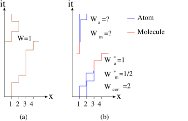
Figure 2: (Color online) Example of world lines for a four-site lattice with periodic boundary conditions. (a) For a system without conversion between the different species, the world lines are continuous and the winding number is well-defined. (b) The conversion between atoms and molecules leads to discontinuities in the world lines, and no true winding can be defined for each of the species. However it is well-defined for the mixture atoms/molecules, because the composite world lines are continuous (see text for details).

V Numerical results

V.1 The one-site problem

It is useful to start the investigation of the model by considering first the one-site problem with a total number of particles $N=2$ ($\rho_{tot}=2$). Figure 3 shows the atomic and molecular densities as functions of the conversion parameter $g$ and different values of the detuning $D$ for $U_{aa}=4$ (the value of $U_{am}$ does not play any role since there is only 2 atoms or 1 molecule). For $D=0$ and small $g$, the 2 particles are mainly bound in the molecular state, because the creation of the molecule has a vanishing energy cost while having 2 atoms costs $2U_{aa}=8$. As $g$ increases, it becomes energetically favorable to make conversions atoms/molecule, so the atomic density starts to grow, reducing the molecular density. When $g$ is large, the system maximizes the conversion process. Thus the system is in the molecular state with 1 molecule half of the time, and in the atomic state with 2 atoms the rest of the time. As a result, the atomic and molecular densities converge to $\rho_{a}=\rho_{tot}/2=1$ and $\rho_{m}=\rho_{tot}/4=1/2$. For $D=6$ the same behavior holds, but the molecular density decreases faster to the large $g$ limit because the energy associated to the molecular state is higher and closer to that of the atomic state. For $D=10$ we have the inverse behavior, the molecular density increases with $g$ and the atomic density decreases, because it is now cheaper energetically to have 2 atoms rather than 1 molecule. The transition point between those two cases is $D=8=2U_{aa}$ for which the atomic state has exactly the same energy as the molecular state. Those states have the same probability, and varying $g$ just changes the rate of conversion between them. Thus the expectation values of the atomic and molecular densities do not depend on the value of $g$, and remain equal to the values that optimize the conversion process: $\rho_{a}=1$ and $\rho_{m}=1/2$.

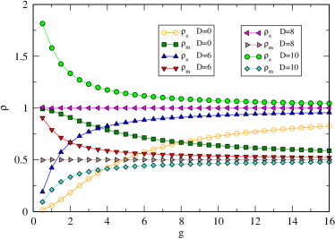
Figure 3: (Color online) The one-site problem with 2 particles. The densities of atoms and molecules are plotted as functions of the conversion parameter $g$ for differents values of the detuning $D$, for $U_{aa}=4$.

V.2 The lattice problem

We now turn to the full problem with $L$ lattice sites. We have performed simulations for $L=20,40,80,160$ and determined by extrapolation to $L=\infty$ that finite size effects associated to the choice of working with $L=20$ lead to errors smaller than our statistical error bars, these latter being smaller than the size of the symbols displayed in the figures of this paper (unless otherwise stated). In the same manner, we have determined that using $\beta=L$ allows to get the physics relevant to the ground state ($\beta=\infty$), for the measured quantities. As for the one-site problem, we start by looking at the atomic and molecular densities as functions of $g$, for different values of the detuning $D$, with $U_{aa}=4$, $U_{am}=12$, and $\rho_{tot}=2$ (Fig. 4). We can see that going from $L=1$ to $L=20$ (equivalent to turning on the hopping parameters $t_{a}$ and $t_{m}$) just leads to small differences at small $g$. For large $g$ the hopping can be neglected, and results for $L=20$ converge to those for $L=1$. Nevertheless it is crucial to keep working with the full lattice problem instead of the one-site problem, since this is required to access global quantities such as the superfluid density. It is also the only way to get results for nearly-continuous values of $\rho_{tot}$.

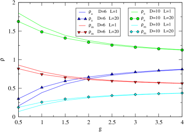
Figure 4: (Color online) The atomic and molecular densities as functions of the conversion parameter $g$ and different values of the detuning $D$, for $U_{aa}=4$, $U_{am}=12$, and total density of particles $\rho_{tot}=2$.

A completely different behavior occurs when considering a non-commensurate density, for instance $\rho_{tot}=4/5$ (Fig. 5). We consider here the case $D<2U_{aa}$ for simplicity. For this density, atoms can be placed on the lattice without increasing the interaction energy. The same holds for the molecules if $D\leq 0$. But for small $g$ and $D\geq 0$ it is energetically more favorable to have atoms only, because 2 atoms have kinetic energy 4 times more negative than 1 molecule ($2(-t_{a})=4(-t_{m})$). As a result the molecular density is vanishing for $g=0$ and $D\geq 0$ and grows when turning on $g$, until reaching the optimal density for large $g$, $\rho_{m}=\rho_{tot}/4=1/5$, in contrast to Fig. 4, where for $D\leq 6$ the density $\rho_{m}$ decreases with increasing $g$. The atomic density follows the inverse behavior, starts for $\rho_{a}=\rho_{tot}$ and converges to the optimal value, $\rho_{a}=\rho_{tot}/2=2/5$.

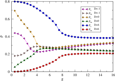
Figure 5: (Color online) The atomic and molecular densities as functions of the conversion parameter $g$ at different values of the detuning $D$. $U_{aa}=4$, $U_{am}=12$, and total density of particles $\rho_{tot}=4/5$.

Having analyzed the system for two specific values of the total density, it is now interesting to perfom a scan of all values of $\rho_{tot}$. Figure 6 shows the atomic and molecular densities as functions of the total density $\rho_{tot}$. At low filling, the particles are dilute and the on-site repulsion between atoms prevent double occupancies, so no binding between atoms can occur and the number of molecules remains zero for all values of $D$ considered. Thus the atomic density increases linearly with the total density. As the filling increases, double occupancies occur leading to the creation of molecules, and decreasing the atomic density. Increasing the filling further leads to an ”inversion of population” where the number of molecules is greater than the number of atoms. This inversion of population is optimal at $\rho_{tot}=2$ for the chosen parameters because double atomic occupancies have an energy cost of $2U_{aa}=8$, whereas the creation of a molecule has an energy cost of $D$. Adding more particles to the system produces a saturation of molecules, and extra atoms just see a constant potential.

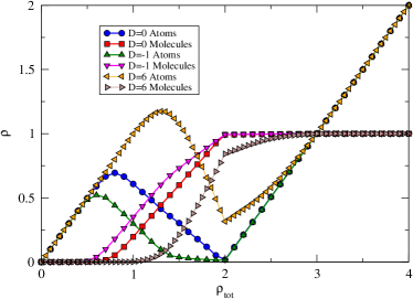
Figure 6: (Color online) The densities of atoms and molecules as functions of the total density $\rho_{tot}$ at different values of the detuning $D$. $U_{aa}=4$, $U_{am}=12$, and $g=0.5$.

In order to identify incompressible phases, it is useful to look at behavior of $\rho_{tot}(\mu)$ for different values of $D$ and $g$ (Fig. 7). Let us recall that the slope of this curve, $\partial\rho/\partial\mu$, is proportional to the isothermal compressibility $\kappa_{T}$. Thus each horizontal plateau indicates an incompressible Mott phase. This does not imply that this phase is insulating, as will be shown below. For $D=-1$ or $D=0$ and small conversion $g=0.5$ one can identify two incompressible phases by the presence of Mott plateaus at $\rho_{tot}=2$ and $\rho_{tot}=3$. For those parameters the usual Mott plateau occuring in pure bosonic systems at $\rho_{tot}=1$ is absent. This is because extra particles can be added beyond $\rho_{tot}=1$ without the need of creating double occupancies, by converting atoms into molecules. For $\rho_{tot}=2$, the phase is incompressible because any site is occupied by a molecule. Thus adding an extra atom requires the formation of an atom/molecule pair, which has an energy cost of $U_{am}$. For $\rho_{tot}=3$, each site is occupied with an atom/molecule pair, and adding extra atoms leads to double occupancies with energy costs of $U_{aa}$. Thus the phase is also incompressible. For $D=6$ and $g=0.5$, we recover a Mott plateau at $\rho_{tot}=1$ because creating a molecule has an energy cost of $D$ that cannot be overcome by the associated negative kinetic and conversion energies. For large $g$ however, the Mott plateaus at $\rho_{tot}=1$ and $\rho_{tot}=3$ disappear. Indeed, in this regime the conversions between atoms and molecules occur and overcome the energy cost of having two atoms on a single site, as well as the energy cost of creating a molecule. Thus extra atoms at $\rho_{tot}=1$ and $\rho_{tot}=3$ can go either into a molecule or doubly occupied sites, without changing the energy by a value greater than the finite-size-lattice gap, which vanishes in the thermodynamic limit. However $\rho_{tot}=2$ is still incompressible because any site is occupied either by two atoms or by a molecule. Thus an extra atom can go only on a site occupied by a molecule, leading to an energy cost of $U_{am}$. Moreover a conversion process can no longer take place on this site, and the system has to pay the price of having a molecule all the time with the associated chemical potential $D$. This explains the large width of the corresponding Mott plateau: approximately $D+g+U_{am}$.

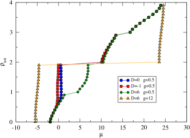
Figure 7: (Color online) The total density as a function of the chemical potential, and different values of $D$ and $g$, for $U_{aa}=4$, and $U_{am}=12$. The slope of these curves is proportional to the isothermal compressibility, and horizontal plateaus indicate phases that are incompressible but not necessarily insulating (see text).

We now study the potential superfluidity of the mixture by analysing the fluctuations of the atomic and molecular pseudo windings $\big{\langle}W_{a}^{\star 2}\big{\rangle}$ and $\big{\langle}W_{m}^{\star 2}\big{\rangle}$, and the correlated and anti-correlated windings $\big{\langle}W_{cor}^{2}\big{\rangle}$ and $\big{\langle}W_{ant}^{2}\big{\rangle}$ (Fig. 8), defined in section IV. To discuss the results, it is useful to consider the corresponding curve in Fig. 7 ($D=6$, $g=0.5$; green curve). For $\rho_{tot}=1$ and $\rho_{tot}=3$ all windings and pseudo windings vanish, showing that the system is frozen for those densities. The corresponding phases are Mott insulators. However for $\rho_{tot}=2$ only the correlated winding vanishes, meaning that there is no global flow of particles, regardless of being atoms or molecules. But individual species are flowing, each in the opposite direction of the other, leading to a large value of the anti-correlated winding. The phase is incompressible like a Mott insulator, but a supercurrent occurs for each of the species. We will refer to this phase as ”Super-Mott”. We show in the following that this phase extends deep into the large-$g$ region of the phase diagram.

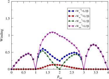
Figure 8: (Color online) The winding as a function of the filling for $U_{aa}=4$, $U_{am}=12$, $g=0.5$, and $D=6$. Error bars of the order of the symbol sizes.

V.3 Phase diagrams

Finally, by reproducing Fig.7 for different sets of parameters $g$ and $D$ we are able to draw two phase diagrams, one in the $(\mu,g)$-plane (Fig. 9) and one in the $(\mu,D)$-plane (Fig. 10). We can identify the three incompressible phases discussed above, namely two Mott phases for $\rho_{tot}=1$ and $\rho_{tot}=3$, and the Super-Mott phase for $\rho_{tot}=2$. Those phases extend over regions of the phase diagram separated by superfluid regions. For small $g$, all incompressible phases are present. As $g$ increases, the Super-Mott phase takes over the two Mott phases (Fig. 9). For small or negative $D$ the Super-Mott phase takes over the $\rho_{tot}=1$ Mott phase, whereas for large $D$ it is the $\rho_{tot}=3$ Mott phase which yields to the Super-Mott phase (Fig. 10).

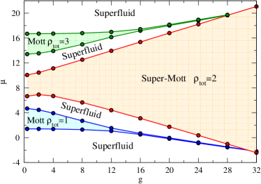
Figure 9: (Color online) The phase diagram in the $(\mu,g)$ plane, for $U_{aa}=4$, $U_{am}=12$, and $D=6$.

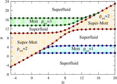
Figure 10: (Color online) The phase diagram in the $(\mu,D)$ plane, for $U_{aa}=4$, $U_{am}=12$, and $g=0.5$.

VI Summary and discussion

We have studied a two-species Bose-Hubbard model including a conversion term between the two species. Our model can be of interest for ultracold atom experiments using Feshbach resonances. The competition between the kinetic, potential, and conversion terms leads to rich phase diagrams. We have shown that increasing the number of particles of the first species can lead to an inversion of population, resulting in the number of molecules greater than the number of atoms. In addition to the usual superfluid and Mott phases occuring in boson models, we have identified an exotic ”Super-Mott” phase, characterized by a vanishing compressibility and a superflow of both species but with anticorrelations such that there is no global supercurrent. Finally, we have produced two phase diagrams as a potential guide to detect the exotic Super-Mott phase. Since the Super-Mott phase occupies a big part of the phase diagrams, we expect it to be observable in experiments. We are currently investigating the model using a newly developed algorithm SGF that provides access to Green functions and momentum distribution functions, which can be measured in experiments. This will allow a direct comparison between theory and experiments.

- (1) M.P.A. Fisher, P.B. Weichman, G. Grinstein, and D.S. Fisher, Phys. Rev. B 40, 546 (1989).
- (2) D. Jaksch, C. Bruder, J.I. Cirac, C.W. Gardiner, and P. Zoller, Phys. Rev. Lett. 81, 3108 (1998).
- (3) H. Ott, E. de Mirandes, F. Ferlaino, G. Roati, G. Modugno, and M. Inguscio, Phys. Rev. Lett. 92, 160601 (2004).
- (4) K. Günter, T. Stöferle, H. Moritz, M. Köhl, T. Esslinger, Phys. Rev. Lett. 96, 180402 (2006).
- (5) S. Ospelkaus, C. Ospelkaus, L. Humbert, K. Sengstock, and K. Bongs, Phys. Rev. Lett. 97, 120403 (2006).
- (6) L. Pollet, M. Troyer, K. Van Houcke, and S.M.A. Rombouts, Phys. Rev. Lett. 96, 190402 (2006).
- (7) P. Sengupta and L.P. Pryadko, Phys. Rev. B 75, 132507 (2007).
- (8) F. Hébert, F. Haudin, L. Pollet, and G.G. Batrouni, Phys. Rev. A 76, 043619 (2007).
- (9) E. Timmermans, P. Tommasini, M. Hussein, and A. Kerman, Physics Reports 315, 199 (1999).
- (10) D.B.M. Dickerscheid, U. Al Khawaja, D. van Oosten, and H.T.C. Stoof, Phys. Rev. A 71, 043604 (2005).
- (11) V. Gurarie, Phys. Rev. A 73, 033612 (2006).
- (12) K. Sengupta and N. Dupuis, Europhys. Lett. 70, 586 (2005).
- (13) G.G. Batrouni, R.T. Scalettar, and G.T. Zimanyi, Phys. Rev. Lett. 65, 176 (1990).
- (14) G.G. Batrouni and R.T. Scalettar, Phys. Rev. B 46, 9051 (1992).
- (15) A.W. Sandvik, J. Phys. A 25, 3667 (1992); Phys. Rev. B 59, R14 157 (1999).
- (16) V.G. Rousseau, R.T. Scalettar, and G.G. Batrouni, Phys. Rev. B 72, 054524 (2005).
- (17) E.L. Pollock, and D.M. Ceperley, Phys. Rev. B 36, 8343 (1987).
- (18) V.G. Rousseau, arXiv:0711.3839