Global classification of two-component approximately integrable evolution equations

Abstract

We globally classify two-component evolution equations, with homogeneous diagonal linear part, admitting infinitely many approximate symmetries. Important ingredients are the symbolic calculus of Gel’fand and Dikiĭ, the Skolem–Mahler–Lech theorem, results on diophantine equations in roots of unity by F. Beukers, and an algorithm of C.J. Smyth.

1 Introduction

A long standing open problem is the classification, up to linear transformations, of two-component integrable equations

$$\left(\begin{array}[]{c}u_{t}\\ v_{t}\end{array}\right)=\left(\begin{array}[]{c}au_{n}+F(u,v,u_{1},v_{1},\ldots)\\ bv_{n}+G(u,v,u_{1},v_{1},\ldots)\end{array}\right)$$ (1)

where $F,G$ are purely nonlinear polynomials in variables $u_{i},v_{i}$, which denote the $i$-th $x$-derivatives of $u(x,t),v(x,t)$. Among the many different approaches to recognition and classification of integrable equations, the so called symmetry approach has proven to be particularly successful, see for example [25, 40] and references in there. Until recently, all results obtained were for classes of equations at fixed (low) order $n$. This situation changed dramatically when, by using a symbolic calculus and results from number theory, Sanders and Wang classified scalar evolution equations with respect to symmetries globally, that is, where the order $n$ can be arbitrarily high [34]. Our aim is to obtain a similar result for the class of multi-component equations (1).

In the symmetry approach the existence of infinitely many generalized symmetries is taken as the definition of integrability. A generalized symmetry of equation (1) is a pair of differential polynomials $S=(S_{1},S_{2})$ such that equation (1) is also satisfied by $\tilde{u}=u+\epsilon S_{1}$, $\tilde{v}=v+\epsilon S_{2}$ up to order $\epsilon^{2}$. This leads to the notion of Lie-derivative: ${\mathcal{L}}(K)S=0$ $\Leftrightarrow$ $S$ is a symmetry of $(u_{t},v_{t})=K$.

The Lie algebra of pairs of differential polynomials is a graded algebra. The linear part $(au_{n},bv_{n})$ has total grading $0$, the quadratic terms have total grading $1$, and so on. Gradings are used to divide the condition for the existence of a symmetry into a number of simpler conditions: ${\mathcal{L}}(K)S\equiv 0$ modulo quadratic terms, ${\mathcal{L}}(K)S\equiv 0$ modulo cubic terms, and so on. This has been called the perturbative symmetry approach [21]. In the same spirit the idea of an approximate symmetry was defined [23]. If ${\mathcal{L}}(K)S\equiv 0$ modulo cubic terms, we say that $S$ is an approximate symmetry of degree 2. And, we call an equation approximately integrable if it has infinitely many approximate symmetries.

We contribute to the above mentioned problem by globally classifying equations (1) that are approximately integrable of degree 2. This is achieved by applying the techniques developed in the special case of so called ${\mathcal{B}}$-equations, where any approximate symmetry of degree 2 is a genuine symmetry [12]. It extends older results obtained by Beukers, Sanders and Wang [2, 3]. See [17] for an overview on the application of number theory in the analysis of integrable evolution equations and [24] for more recent results. The present article is a revised and extended version of the report [13].

As remarked in [23] the requirement of the existence of approximate symmetries of degree $2$ is very restrictive and highly non-trivial. On the other hand an equation may have infinitely many approximate symmetries of degree $2$, but fail to have any symmetries. This problem involves conditions of higher grading and is left open.

2 Generalized symmetries

A symmetry-group transforms one solution to an equation to another solution of the same equation. We refer to the book of Olver [29] for an introduction to the subject, numerous examples and applications.

We denote ${\mathcal{A}}=\mathbb{C}[u,v,u_{1},v_{1},\ldots]$ and ${\mathfrak{g}}={\mathcal{A}}\otimes{\mathcal{A}}$. We will endow ${\mathfrak{g}}$ with the structure of a Lie algebra. For any $K=(K_{1},K_{2})\in{\mathfrak{g}}$ the pair $S=(S_{1},S_{2})\in{\mathfrak{g}}$ is a generalized symmetry of the two-component evolution equation

$$\left(\begin{array}[]{c}u_{t}\\ v_{t}\end{array}\right)=\left(\begin{array}[]{c}K_{1}\\ K_{2}\end{array}\right)$$ (2)

if the Lie derivative of $S$ with respect to $K$,

$${\mathcal{L}}(K)S=\left(\begin{array}[]{c}\delta_{K}(S_{1})-\delta_{S}(K_{1})\\ \delta_{K}(S_{2})-\delta_{S}(K_{2})\end{array}\right),$$ (3)

vanishes. Here $\delta_{Q}$ is the prolongation of the evolutionary vector field with characteristic $Q$, cf. [29, equation 5.6],

$$\delta_{(Q_{1},Q_{2})}=\sum_{k=0}^{\infty}D_{x}^{k}Q_{1}\frac{\partial}{\partial u_{k}}+D_{x}^{k}Q_{2}\frac{\partial}{\partial v_{k}},$$

and the total derivative $D_{x}$ is

$$D_{x}=\sum_{k=0}^{\infty}u_{k+1}\frac{\partial}{\partial u_{k}}+v_{k+1}\frac{\partial}{\partial v_{k}}.$$

The Lie derivative is a representation of ${\mathfrak{g}}$. This property, with $P,Q\in{\mathfrak{g}}$,

$${\mathcal{L}}({\mathcal{L}}(P)Q)={\mathcal{L}}(P){\mathcal{L}}(Q)-{\mathcal{L}}(Q){\mathcal{L}}(P)$$ (4)

corresponds to the Jacobi identity for the Lie bracket $[P,Q]={\mathcal{L}}(P)Q$ which is clearly bilinear and antisymmetric, cf. [29, Proposition 5.15]. Another way of expressing (4) is saying that ${\mathfrak{g}}$ is a ${\mathfrak{g}}$-module. Another ${\mathfrak{g}}$-module is given by ${\mathcal{A}}$, the representation being ${\mathcal{L}}(K)F=\delta_{K}(F)$ with $K\in{\mathfrak{g}},F\in{\mathcal{A}}$.

The word ‘generalized’ stresses the fact that the order of a symmetry can be bigger than one. Generally symmetries come in hierarchies with periodic gaps between their orders. For example, the Korteweg–De Vries equation $u_{t}=u_{3}+uu_{1}$ possesses odd order symmetries only. Concurrently, the KDV equation has approximately symmetries at any order.

3 Grading

Denote $\sigma_{u}=(u,0)$ and $\sigma_{v}=(0,v)$. If $P$ in some ${\mathfrak{g}}$-module is an eigenvector of ${\mathcal{L}}(\sigma_{u})$ (or of ${\mathcal{L}}(\sigma_{v})$), the corresponding eigenvalue is called the $u$- (or $v$-) grading of $P$. If $P$ has $u$-grading $i$ and $v$-grading $j$ we say that $i+j$ is the total grading of $P$. One verifies that ${\mathfrak{g}}$ can be written as the direct sum

$${\mathfrak{g}}=\bigoplus_{t\geq 0}{\mathfrak{g}}^{t},\quad{\mathfrak{g}}^{t}=\bigoplus_{-1\leq i\leq t+1}{\mathfrak{g}}^{i,t-i},$$

where elements of ${\mathfrak{g}}^{i,j}$ have $u$-grading $i$ and $v$-grading $j$. For example, $(u_{1}v_{2},v_{3}v_{4})\in{\mathfrak{g}}^{0,1}$ has total grading 1. Similarly we have

$${\mathcal{A}}=\bigoplus_{t\geq 0}{\mathcal{A}}^{t},\quad{\mathcal{A}}^{t}=\bigoplus_{0\leq i\leq t}{\mathcal{A}}^{i,t-i}.$$

The crucial property of a graded Lie algebra is that the $u$-, (or $v$-, or total) grading of ${\mathcal{L}}(P)Q$ is the sum of the $u$-, (or $v$-, or total) gradings of $P$ and $Q$. This follows directly from equation (4). Gradings are used to divide the condition for the existence of a symmetry into a number of simpler conditions.

We study evolution equations of the form

$$\left(\begin{array}[]{c}u_{t}\\ v_{t}\end{array}\right) = K^{0}+K^{1}+\cdots$$ (7)

$$= K^{0,0}+K^{-1,2}+K^{0,1}+K^{1,0}+K^{2,-1}+\cdots,$$ (8)

with $K^{0,0}=(au_{n},bv_{n})$ and symmetries of similar form $S=S^{0}+S^{1}+\cdots$ with $S^{0}=S^{0,0}=(cu_{m},dv_{m})$. Here the dots may contain terms with total grading $>1$. Certainly we have ${\mathcal{L}}(K^{0,0})S^{0,0}=0$. The symmetry conditions with total grading 1 are

$${\mathcal{L}}(K^{-1,2})S^{0,0}+{\mathcal{L}}(K^{0,0})S^{-1,2} =0,$$

$${\mathcal{L}}(K^{0,0})S^{0,1}+{\mathcal{L}}(K^{0,1})S^{0,0} =0,$$

$${\mathcal{L}}(K^{0,0})S^{1,0}+{\mathcal{L}}(K^{1,0})S^{0,0} =0,$$

$${\mathcal{L}}(K^{0,0})S^{2,-1}+{\mathcal{L}}(K^{2,-1})S^{0,0} =0.$$

An implicit function theorem which, under certain conditions, guarantees that $S$ is a symmetry of $K$ if the first few symmetry conditions of total grading $0,1,\ldots$ are fulfilled, was given by Sanders and Wang [34, 35]. In this paper we restrict ourselves to solving equations (3). Thus we classify equations that admit infinitely many approximate symmetries of degree 2, which is a necessary condition for integrability. In the sequel we omit the adjective ‘of degree 2’.

4 The Gel’fand–Dikiĭ transformation

Comparing the Leibniz rule and Newton’s binomial formula,

$$(uv)_{n}=\sum_{i=0}^{n}\binom{n}{i}u_{i}v_{n-i},\qquad(x+y)^{n}=\sum_{i=0}^{n}\binom{n}{i}x^{i}y^{n-i},$$

we see that differentiating a product is quite similar to taking the power of a sum. On the right hand side the index, counting the number of derivatives, gets interchanged with the power, while on the left hand side differentiation becomes multiplying with the sum of symbols. Of course, with expressions containing both indices and powers, one has to be more careful. The Gel’fand–Dikiĭ transformation [10] provides a one to one correspondence between ${\mathcal{A}}^{i,j}$ and the space $\mathbb{C}^{i,j}$: polynomials in $\mathbb{C}[x_{1},\ldots,x_{i},y_{1},\ldots,y_{j}]$ that are symmetric in both the $x$ and the $y$ symbols. One may deduce the general rule from

$$u_{1}u_{2}v_{3}\trianglerighteq\frac{x_{1}^{1}x_{2}^{2}+x_{2}^{1}x_{1}^{2}}{2!}\frac{y_{1}^{3}}{1!}=\widehat{u_{1}u_{2}v_{3}},$$

or consult one of the papers [17, 21, 24]. All usual operations from differential algebra translate naturally. In particular,

$${\mathcal{L}}(K^{0,0})S^{i,j}\trianglerighteq\left(\begin{array}[]{cc}{\mathcal{G}}^{i,j}_{1;n}[a{,}b]&0\\ 0&{\mathcal{G}}^{i,j}_{2;n}[a{,}b]\end{array}\right)\widehat{S^{i,j}},$$

where the so called ${\mathcal{G}}$-functions are given by

$${\mathcal{G}}^{i,j}_{1;n}[a{,}b](x,y) = a(x_{1}^{n}+\cdots+x_{i+1}^{n})+b(y_{1}^{n}+\cdots+y_{j}^{n})$$

$$-a(x_{1}+\cdots+x_{i+1}+y_{1}+\cdots+y_{j})^{n},$$

and

$${\mathcal{G}}^{i,j}_{2;n}[a{,}b](x,y)={\mathcal{G}}^{j,i}_{1;n}[b{,}a](y,x).$$ (10)

Symbolically we can solve the symmetry conditions of total grading 1, equations (3), as follows. We may write the components of the quadratic parts of $S$ as, with $k=1,2$,

$$\widehat{S^{i,j}_{k}}=\frac{{\mathcal{G}}^{i,j}_{k;m}[c{,}d]}{{\mathcal{G}}^{i,j}_{k;n}[a{,}b]}\widehat{K^{i,j}_{k}}.$$ (11)

Equation (8) has an approximate symmetry at order $m$ with linear coefficients $c,d$ iff for all $i+j=1$ and $k=1,2$ the right hand side of equation (11) is either polynomial or undefined ($0/0$).

5 Nonlinear injectivity

In our classification we distinguish between equations whose approximate symmetries necessarily have non-vanishing linear part and equations that allow purely nonlinear approximate symmetries.

Definition 1

Let $K^{0}$ have total grading 0. We call $K^{0}$ nonlinear injective if ${\mathcal{L}}(K^{0})S=0$ implies that $S$ has total grading 0. And, we call an equation nonlinear injective if its linear part is nonlinear injective.

With $K^{0}=(au_{n},bv_{n})$, the $k$-th component of ${\mathcal{L}}(K^{0})S^{i,j}$, with non-zero $S^{i,j}$, vanishes iff ${\mathcal{G}}^{i,j}_{k,n}[a{,}b]=0$. Solving the later equation with $i+j=1$ yields $ab=0$, $n\geq 0$, or $n=1$, or $(a-2b)(2a-b)=0$, $n=0$. In Table 1 we have displayed all $K^{0}$ and corresponding $S^{1}$, such that the equation $(u_{t},v_{t})=K^{0}+K^{1}$, with arbitrary $K^{1}\in{\mathfrak{g}}^{1}$, has purely nonlinear approximate symmetries $S^{1}\in{\mathfrak{g}}^{1}$. Note that the classification is performed up to linear transformations. In particular we may interchange $u$ and $v$. Therefore without loss of generality we set $b=1$ and classify the values of $a$ up till inversion.

$K^{0}$	$(0,v)$	$(2u,v)$	$(au_{1},v_{1}),a\neq 1$	$(u_{1},v_{1})$	$(0,v_{n})$, $n>1$
$S^{1}$	${\mathfrak{g}}^{1,0}$	${\mathfrak{g}}^{-1,2}$	${\mathcal{A}}^{2,0}\otimes{\mathcal{A}}^{0,2}$	${\mathfrak{g}}^{1}$	${\mathcal{A}}^{2,0}\otimes 0$

Table 1: List of $K^{0}$ and $S^{1}$ such that ${\mathcal{L}}(K^{0})S^{1}=0$.

For the same choices of $K^{0}$ and $S^{1}$ the linear equation $(u_{t},v_{t})=K^{0}$ has symmetries $(cu_{m},dv_{m})+S^{1}$ for all $m\in\mathbb{N}$ and $c,d\in\mathbb{C}$. Indeed, every ${\mathcal{B}}$-equation, that is, an equation of the form (8) with $K^{1}\in{\mathfrak{g}}^{-1,2}$, admits the zeroth order symmetry $(2u,v)$. In fact, every tuple $S\in{\mathfrak{g}}$ is a symmetry of $(u_{t},v_{t})=(u_{1},v_{1})$. Or, in other words, $(u_{1},v_{1})$ is a symmetry of every equation.

Only a subset of the equations $(u_{t},v_{t})=K^{0}+K^{1}$, with particular $K^{1}\in{\mathfrak{g}}$, has infinitely many symmetries with non-vanishing linear part. There is a good reason for including such equations in the classification: their approximate symmetries may correspond to approximately integrable nonlinear injective equations. One integrable example, equation (40), is given in section 11. On the other hand, nonlinear injectivity is one of the conditions in the implicit function theorem of Sanders and Wang, see section 3.

6 Necessary and sufficient conditions

In this section we introduce convenient notation, we give necessary and sufficient conditions for a nonlinear injective equation to be approximately integrable, and we outline how we perform the classification.

The components of equation (8) are

$$\left(\begin{array}[]{c}u_{t}\\ v_{t}\end{array}\right)=\left(\begin{array}[]{c}au_{n}+K_{1}^{1,0}+K_{1}^{0,1}+K_{1}^{-1,2}+\cdots\\ bv_{n}+K_{2}^{0,1}+K_{2}^{1,0}+K_{2}^{2,-1}+\cdots\end{array}\right).$$ (12)

We denote the symbolic representation of the 6-tuple $K_{1}^{1,0}$, $K_{1}^{0,1}$, $K_{1}^{-1,2}$, $K_{2}^{0,1}$, $K_{2}^{1,0}$, $K_{2}^{2,-1}$ by $\widehat{K}^{1}$. And similarly we write $S_{1}^{1,0}$, $\ldots$, $S_{2}^{2,-1}\trianglerighteq\widehat{S}^{1}$ and ${\mathcal{G}}_{n}={\mathcal{G}}_{1;n}^{1,0},\ldots,{\mathcal{G}}_{2;n}^{2,-1}$. A $6$-tuple $H$ is called proper if it consists of polynomials with the right symmetry properties, that is, if $H\in\mathbb{C}^{2,0}\otimes\mathbb{C}^{1,1}\otimes\mathbb{C}^{0,2}\otimes\mathbb{C}^{0,2}\otimes\mathbb{C}^{1,1}\otimes\mathbb{C}^{2,0}$. Thus, $\widehat{K}^{1}$, $\widehat{S}^{1}$, and ${\mathcal{G}}_{n}[a{,}b]$ are proper tuples. We will also consider $s$-tuples, with $s<6$. It should be clear from the context in which space a proper $s$-tuple lives. We say that an $s$-tuple $H=H_{[1]},\ldots,H_{[s]}$ divides an $s$-tuple $P=P_{[1]},\ldots,P_{[s]}$ if $H_{[i]}\mid P_{[i]}$ for all $1\leq i\leq s$ and we write $P/H=P_{[1]}/H_{[1]},\ldots,P_{[s]}/H_{[s]}$. We are now able to state the following: Equation (12) is nonlinear injective and has an approximate symmetry of order $m$ with linear coefficients $c,d$ iff the 6-tuple $\widehat{S}^{1}={\mathcal{G}}_{m}[c{,}d]\widehat{K}^{1}/{\mathcal{G}}_{n}[a{,}b]$ is proper.

Let $H$, ${\mathcal{G}}_{m}[c,d]$ be proper $s$-tuples. With $m(H)$ we denote the set of all $m\in\mathbb{N}$ such that there exists $c,d\in\mathbb{C}$ for which $H\mid{\mathcal{G}}_{m}[c{,}d]$. And, the set of all proper $s$-tuples $H$ with infinite $m(H)$ will be denoted ${\mathcal{H}}^{s}$, or simply ${\mathcal{H}}$ when it is clear from the context what $s$ is. We organize $H\in{\mathcal{H}}$ by the lowest order $n$ at which $H$ divides a ${\mathcal{G}}_{n}$-tuple. By ${\mathcal{H}}_{n}$ we denote the set of all proper tuples $H$ with infinite $m(H)$ whose smallest element is $n$.

We have the following lemma.

Lemma 2

Equation (12) is nonlinear injective and approximately integrable iff there is a proper 6-tuple $H$ with $m(H)$ infinite, such that ${\mathcal{G}}_{n}[a{,}b]$ divides $\widehat{K}^{1}H$.

Proof:

• The fact that ${\mathcal{G}}_{n}[a{,}b]$ divides a proper tuple implies that equation (12) is nonlinear injective. The equation is approximately integrable because for every $m\in m(H)$ there are $c,d$ such that

  $$\widehat{S}^{1}=\frac{{\mathcal{G}}_{m}[c{,}d]}{H}\frac{\widehat{K}^{1}H}{{\mathcal{G}}_{n}[a{,}b]}$$

  is proper.

• Because equation (12) is nonlinear injective, the tuple $\widehat{S}^{1}={\mathcal{G}}_{m}[c{,}d]\widehat{K}^{1}/{\mathcal{G}}_{n}[a{,}b]$ is well defined for all $m$. The integrability implies that $S^{1}$ is proper for infinitely many $m\in\mathbb{N}$ and $c,d\in\mathbb{C}$. This only happens when ${\mathcal{G}}_{n}=HP$ factorizes such that $P\mid\widehat{K}^{1}$ and $m(H)$ is infinite. $\square$
  

According to Lemma 2, to classify approximately integrable nonlinear injective equations it suffices to determine the set ${\mathcal{H}}^{6}$ of all proper 6-tuples $H$ with infinite $m(H)$. This will be done using results from number theory, provided in section 7. In section 8 we determine the proper divisors $H\in{\mathcal{H}}^{1}$ of infinitely many functions ${\mathcal{G}}^{i,1-i}_{k,m}$ for possible $i,k$. And, in section 9 we determine the proper divisors $H\in{\mathcal{H}}^{2}$ of infinitely many 2-tuples ${\mathcal{G}}^{i,1-i}_{1,m}$, ${\mathcal{G}}^{j,1-j}_{k,m}$, where $i\neq j$ if $k=1$. From those results we determine the set ${\mathcal{H}}^{6}=\bigcup_{n\in\mathbb{N}}{\mathcal{H}}^{6}_{n}$ in section 10. For each $n\in\mathbb{N}$ the set ${\mathcal{H}}_{n}$ is related to the set of approximate integrable equations at order $n$, which are not in a lower order hierarchy.

We would like to provide an explicit but minimal list of approximate integrable equations from which one can derive all approximately integrable equations. The following observation is useful. Let $P$ and $Q$ be proper tuples. From Lemma 2 it follows that if equation (12), with $\widehat{K}^{1}=P$, is approximately integrable, then the same equation, but with $\widehat{K}^{1}=PQ$, is also approximately integrable. Therefore, the classification in section 10 describes the divisors that have maximal degree. And the corresponding list of equations only contains equations with quadratic parts $K^{1}$ of minimal degree.

From the results of sections 8, 9 it follows that ${\mathcal{H}}_{n}$ is non-empty for all $n\in\mathbb{N}$. That means there are new approximately integrable equations at every order. In section 10 we classify the highest degree divisors in ${\mathcal{H}}_{n}$ completely, that is, for any order. We are not able to explicitly list all corresponding equations, as this paper is bound to be finite. In section 10 we do provide a complete list of approximately integrable equations of order $n\leq 5$.

We explicitly provide the linear parts $(cu_{m},du_{m})$ of all the symmetries of the equations in our list. This enables one to calculate any approximate symmetry in principle. This can be done using Maple code provided at [15]. We remark that if one multiplies the quadratic tuple of an equation with a proper tuple, the resulting equation may have more symmetries than the original one. As we will now illustrate it may also be in a lower hierarchy.

From Lemma 2 we know that if $H\in{\mathcal{H}}_{n}$ and ${\mathcal{G}}_{n}[a{,}b]\mid\widehat{K}^{1}H$, then equation (12) is approximately integrable with approximate symmetries at (higher) order $m\in m(H)$. The following lemma applies.

Lemma 3

Suppose $H\in{\mathcal{H}}_{n}$ and ${\mathcal{G}}_{n}[a{,}b]$ divides $\widehat{K}^{1}H$. Then equation (12) has more symmetries than the ones at order $m\in m(H)$ iff there is a divisor $Q\in{\mathcal{H}}_{k\leq n}$ of $H$, with $m(H)$ smaller than and contained in $m(Q)$, such that ${\mathcal{G}}_{n}[a{,}b]$ divides $\widehat{K}^{1}Q$.

Proof: Given a divisor $Q\in{\mathcal{H}}_{k}$ of $H$ such that ${\mathcal{G}}_{n}[a{,}b]\mid\widehat{K}^{1}Q$, it is clear that equation (12) has a symmetry at every order $m\in m(Q)$ with

$$\widehat{S}^{1}=\frac{{\mathcal{G}}_{m}[c{,}d]}{Q}\frac{\widehat{K}^{1}Q}{{\mathcal{G}}_{n}[a{,}b]}.$$

To see that the converse holds, let $Y$ denote the set of orders of approximate symmetries, with $m(H)$ smaller than and contained in $Y$. We need to prove that there is a $Q$ such that $Y=m(Q)$. Take $m\in Y\setminus m(H)$ and write ${\mathcal{G}}_{n}=HP$. Since ${\mathcal{G}}_{n}\mid\widehat{K}^{1}H$ we have $\widehat{K}^{1}=PR$. The tuple $\widehat{S}^{1}={\mathcal{G}}_{m}\widehat{K}^{1}/{\mathcal{G}}_{n}={\mathcal{G}}_{m}R/H$ is proper. Since $m\not\in m(H)$, $H$ does not divide ${\mathcal{G}}_{m}$. There is a proper divisor $Q$ of $H$ such that $Q\mid{\mathcal{G}}_{m}$ and $H/Q$ divides $R$, that is, ${\mathcal{G}}_{n}\mid\widehat{K}^{1}Q$. Since $Q\mid H$ the set $m(Q)$ is infinite. $\square$

Remark 4

One can start with an equation that is not nonlinear injective, multiply its quadratic tuple, and end up in the hierarchy of an nonlinear injective equation. For example, apart from certain purely nonlinear symmetries, equation 1.2 has approximately symmetries with linear part $(cu_{m},dv_{m})$ for any $c,d\in\mathbb{C}$ when $m$ is odd. By multiplying its quadratic tuple with the tuple $[0,(f_{1}x_{1}+f_{2}y_{1})/f,(y_{1}+y_{2})/2,0,(i_{1}x_{1}+i_{2}y_{1})/i,(x_{1}+x_{2})/2]$ we obtain the equation

$$\left(\begin{array}[]{c}u_{t}\\ v_{t}\end{array}\right)=\left(\begin{array}[]{c}au_{1}+f_{1}u_{1}v+f_{2}uv_{1}+gvv_{1}\\ v_{1}+i_{1}u_{1}v+i_{2}uv_{1}+juu_{1}\end{array}\right),$$

which has approximate symmetries at all orders $m>0$ for any $c,d\in\mathbb{C}$, and, it is in the hierarchy of an equation of the form 0.3 iff $f_{1}=i_{2}=0$. In this paper we do not explicitly describe all symmetries of all approximately integrable equations that can be obtained from our list.

7 Results from number theory

Generally speaking, progress in classifying global classes of evolution equations has been going hand in hand with applying new results or techniques from number theory. For the classification of scalar equations [34] the new result was obtained by F. Beukers, who applied sophisticated techniques from diophantine approximation theory [1]. The Skolem–Mahler–Lech theorem, stated below, first appeared in the literature in connection with symmetries of evolution equations in [2]. Beukers, Sanders and Wang used a partial corollary of this theorem to conjecture that there are only finitely many integrable equations (12) with $K^{1}=[0,0,1,0,0,0]$. Their conjecture became a theorem in [3], where an exhaustive list of the integrable cases was produced using a recent algorithm of C.J. Smyth [4], that solves polynomial equations $f(x,y)=0$ for roots of unity $x,y$. And, the classification of ${\mathcal{B}}$-equations was due to results on diophantine equations in roots of unity, again proved by Beukers [12].

However, as it turns out, we do not need entirely different results or techniques from number theory to globally classify two component evolution equations, with homogeneous diagonal linear part, admitting infinitely many approximate symmetries.

7.1 The Skolem–Mahler–Lech theorem

A sequence $\{U_{m},m\in\mathbb{N}\}$ satisfies an order $n$ linear recurrence relation if there exist $s_{1},\ldots,s_{n}$ such that

$$U_{m+n}=s_{1}U_{m+n-1}+\cdots s_{n}U_{m}.$$

The general solution can be expressed in terms of a generalized power sum

$$U_{m}=\sum_{i=1}^{k}A_{i}(m)\alpha_{i}^{m},$$

such that the roots $\alpha_{i}$ are distinct and non-zero, and the coefficients $A_{i}(m)$ are polynomial in $m$. By definition the degree of $U_{m}$ is $d=\sum_{i=1}^{k}d_{i}$, where $d_{i}$ is the degree of $A_{i}(m)$. It can be shown that the order of the sequence equals $n=k+d$ [32].

A generalized power sum vanishes identically, $U_{m}=0$ for all $m$, precisely when all its coefficients vanish as polynomials in $m$, $A_{i}(m)=0$ for all $i$. We prove this by induction on the degree. For $d=0$ the statement is plain, the functions $h\rightarrow\alpha_{i}^{h}$ are linearly independent for distinct $\alpha_{i}$. Let $S:f(m)\rightarrow f(m+1)$ be the shift operator. Suppose $d>0$. Then for some $i$ we have $d_{i}>0$. The generalized power sum $V_{m}=(S-\alpha_{i})U_{m}$ has degree $d-1$. By the induction hypothesis we have, in particular, $\alpha_{i}(S-1)A_{i}(h)=0$. Since $\alpha_{i}\neq 0$ this implies $d_{i}=0$ and hence we are done.

Theorem 5 (Skolem–Mahler–Lech)

The zero set of a linear recurrence sequence $\{m\in\mathbb{N}:U_{m}=0\}$ is the union of a finite set and finitely many complete arithmetic progressions.

Note that an arithmetic progression $p$ is complete if $p=\{f+gh:h\in\mathbb{N}\}$ for some remainder $f\in\mathbb{N}_{0}$ and difference $g>f$, $g\in\mathbb{N}$. Theorem 5 was first proved by Skolem for the rational numbers [37], by Mahler for algebraic numbers [19], and by Lech for arbitrary fields of characteristic zero [18]. The proofs rely on $p$-adic analysis and consist of showing the existence of a difference $g\in\mathbb{N}$ such that every partial sum, with $0\leq f<g$,

$$U_{f+gh}=\sum_{i=1}^{k}(A_{k}(f+gh)\alpha_{i}^{f})(\alpha_{i}^{g})^{h}$$ (13)

either has finitely many solutions $h$ or vanishes identically. We refer to [27, 39], and references in there, for sensible sketches of a proof.

If (13) vanishes identically the sum on the right breaks up into disjoint pieces $I\subset\{1,\ldots,m\}$ each of which vanishes because the roots $\alpha_{i}^{g}$, $i\in I$, coincide and the sum of their coefficients $\sum_{i\in I}A_{i}(f+gh)\alpha_{i}^{f}$ vanishes identically as a function of the variable $h$. Since $A_{i}(f+gh)$ does not vanish identically, each piece contains at least two terms. In particular, the following will be usefull.

Corollary 6

If the equation

$$a_{1}\alpha_{1}^{m}+a_{2}\alpha_{2}^{m}+\cdots+a_{k}\alpha_{k}^{m}=0,$$

with nonzero $a_{i},\alpha_{i}\in\mathbb{C}$ has infinitely many solutions, the set $\{\alpha_{1},\alpha_{2},\ldots,\alpha_{k}\}$ partitions into a number of disjoint subsets, such that each subset has at least two members, and the ratio of any two members of a subset is a root of unity.

For instance, when $k=3$ the triple $\alpha_{1}/\alpha_{2},\alpha_{2}/\alpha_{3},\alpha_{1}/\alpha_{3}$ consists of roots of unity.

7.2 Diophantine equations in roots of unity

The following theorems are of crucial importance for the classification problem considered in this paper.

Theorem 7 (Beukers)

Take $m>1$ integer. Let $\mu,\nu$ be distinct roots of unity, both not equal to 1, such that $\nu\neq\mu^{-1}$ when $m$ is odd. Then

$$(1-\nu^{m})(1-\mu)^{m}=(1-\mu^{m})(1-\nu)^{m}$$ (14)

implies $\mu^{m}=\nu^{m}=1$.

Theorem 8 (Beukers)

Take $m>1$ integer. Let $\mu,\nu$ be distinct roots of unity, not both equal to 1, such that $\nu\neq\mu^{-1}$ when $m$ is even. Then

$$(1+\nu^{m})(1-\mu)^{m}=(1+\mu^{m})(1-\nu)^{m}$$ (15)

implies $\mu^{m}=\nu^{m}=-1$.

Theorem 9 (Beukers)

Take $m>1$ integer. Let $\mu,\nu$ be roots of unity with $\mu\neq 1$. Then

$$(1+\nu^{m})(1-\mu)^{m}=(1-\mu^{m})(1-\nu)^{m}$$ (16)

implies $\mu^{m}=-\nu^{m}=1$.

Whereas the Skolem–Mahler–Lech theorem implies that certain ratios are roots of unity for the equation to have infinitely many solutions, the above theorems tell us precisely what the solutions are. In particular, they imply that the zero sets consist of complete arithmetic progressions only.

Theorems 7,8,9 are slightly more general than [12, Theorems 22,25], which were proved by F. Beukers. We won’t repeat their proofs here, however we do indicate the difference between the two sets of Theorems, which is twofold. Firstly, in Theorems 7,8,9 we do not assume that $\mu,\nu\neq-1$. In certain cases this follows from [12, Proposition 24], in others one has to rely on the following.

Proposition 10 (Beukers)

If $\nu$ is a root of unity such that

$$(1+\nu^{m})2^{m-1}=(1-\nu)^{m},$$ (17)

then $\nu=-1$ and $m$ is even.

Proof: By Galois theory we may assume that $\nu=e^{2\pi i/n}$. Taking $n=1$ does not give any solutions. If $n=2$ then $m$ has to be even. We will show there are no solutions with $n>2$. When $m=1$ there is no root of unity such that $1+\nu=1-\nu$. Taking $m=2$ it follows that $n=2$. So we may assume that $m>2$.

Since $\nu\neq 1$, $|1+\nu^{m}|$ does not vanish and we have $|1+\nu^{m}|>\sin(\pi/n)$. Also we use $|1-\nu|<2\pi/n$. This gives

$$(2\frac{\pi}{n})^{m}>|1-\nu|^{m}=|1+\nu^{m}|2^{m-1}>\sin(\frac{\pi}{n})2^{m-1}.$$

Division by $2^{m}\pi/n$ yields (taking $n>2$)

$$(\frac{\pi}{n})^{m-1}>\sin(\frac{\pi}{n})\frac{n}{2\pi}>.41,$$

which implies (taking $m>2$) that $\pi/n>.64$, or $n<5$. When $n=3$, $|1+\nu^{m}|$ equals 1 or 2, and $|1-\nu|=\sqrt{3}$, whose $m$-th power does not equal $2^{m}$ or $2^{m-1}$. When $n=4$, $|1+\nu^{m}|$ equals 0 or $\sqrt{2}$ or $2$, and $|1-\nu|=\sqrt{2}$, whose $m$-th power, with $m>1$, does not equal $0$ or $\sqrt{2}2^{m-1}$ or $2^{m}$. $\square$

Secondly in the proofs we do not in general need $\nu\neq\mu$ and $\nu\neq 1/\mu$. And, we also note that in [12, Theorem 25] it was mistakenly supposed that $\mu^{n}\neq-1$. This should have been $\mu^{n}\neq\mp 1$ depending on the sign in [12, equation (10)].

8 Homogeneous quadratic parts

In this section we determine the proper divisors of infinitely many 1-tuples ${\mathcal{G}}_{m}={\mathcal{G}}^{i,1-i}_{k,m}$ for all possible choices of $i,k$.

Due to equation (10) we may take $k=1$; equations of the form $(u_{t},v_{t})=(au_{n},bv_{n}+K)$ are related, by the linear transformation $u\leftrightarrow v$, to equations of the form $(u_{t},v_{t})=(au_{n}+K,bv_{n})$. We start with the simplest case $i=1$.

8.1 Classifying approximately integrable scalar equations

The Lie derivative of the quadratic part $S^{1}$ of a possible scalar symmetry with respect to the linear part $K^{0}=u_{n}$ of a scalar equation $u_{t}=K^{0}+K^{1}+\cdots$ is symbolically given by ${\mathcal{L}}(K^{0})S^{1}\trianglerighteq G^{1}_{n}\widehat{S}^{1}$ with ${\mathcal{G}}$-function

$${\mathcal{G}}^{1}_{n}(x,y)=x^{n}+y^{n}-(x+y)^{n}={\mathcal{G}}^{1,0}_{1;n}[a{,}b](x,y)/a.$$

Thus the case $i=k=1$ is equivalent to the scalar problem, which is easily seen by taking $v=0$. The function is also proportional to ${\mathcal{G}}^{i,1-i}_{k,n}[a{,}a]$ so the results apply to the case $a=b$ as well.

In the classification of scalar equations [34] a different route was taken than the one we take. Namely, whereas we perform our classification with respect to the existence of infinitely many (approximate) symmetries, Sanders and Wang performed their classification with respect to the existence of symmetries (finitely many or infinitely many). They showed in particular that there are no scalar equations with finitely many generalized symmetries, which confirms the first part of the conjecture of Fokas [8]:

If a scalar equation possesses at least one time-independent non-Lie point symmetry, then it possesses infinitely many. Similarly for $N$-component equations one needs $N$ symmetries.

We note that the conjecture of Fokas does not hold inside the class of ${\mathcal{B}}$-equations [16]. In their classification Sanders and Wang relied on the following ‘hard to obtain’ result from number theory, proved in [1].

Theorem 11 (Beukers)

Let $r\in\mathbb{C}$ such that $r(r+1)(r^{2}+r+1)\neq 0$. Then at most one integer $m>1$ exists such that ${\mathcal{G}}^{1}_{m}(1,r)=0$.

In contrast, classifying the equations with respect to (approximate) integrability can be done using the following ‘easy to obtain’ result. Proposition 12 is of course not as strong as Theorem 11. For obvious reasons we do not include the constant divisors in ${\mathcal{H}}_{0}$ in our lists.

Proposition 12

The proper divisors of infinitely many ${\mathcal{G}}^{1,0}_{1;m}[c{,}d](1,y)$ are products of

1. $y\in{\mathcal{H}}_{2}$, $m>1$

2. $(1+y)\in{\mathcal{H}}_{3}$, $m\equiv 1\mod 2$

3. $1+y+y^{2}\in{\mathcal{H}}_{5}$, $m\equiv 1,5\mod 6$

4. $(1+y+y^{2})^{2}\in{\mathcal{H}}_{7}$, $m\equiv 1\mod 6$

Proof: According to the Skolem–Mahler–Lech theorem, see Corollary (6), if the diophantine equation ${\mathcal{G}}^{1}_{m}(1,r)=0$ has infinitely many solutions $m$, then $r=0,-1$ or $r$ and $r+1$ are both roots of unity, in which case $r$ is a primitive $3$-rd root of unity. The orders are found by substituting the values for $r$. We have ${\mathcal{G}}^{1}_{m}(1,0)=0$ for all $m$, ${\mathcal{G}}^{1}_{f+2h}(1,-1)=1+(-1)^{f}=0$ when $f=1$, and, with $1+r+r^{2}=0$, ${\mathcal{G}}^{1}_{f+6h}(1,r)=1+r^{f}-(1+r)^{f}=0$ when $f=1$ or $f=5$. Finally, by solving the simultaneous equations ${\mathcal{G}}^{1}_{m}(1,r)=\partial_{r}{\mathcal{G}}^{1}_{m}(1,r)=0$ we find that $r$ is a double zero when both $r$ and $1+r$ are $(m-1)$-st roots of unity. $\square$

As a particular corollary of Proposition 12 we have the following. Equation (12) with $a=b$ and $n=2,3,5,7$ is approximately integrable for arbitrary $K^{1}$.

8.2 ${\mathcal{B}}$-equations

The case $i=-1$ has been globally classified with respect to integrability in [12]. This class of equations is particularly nice because any approximate symmetry is a symmetry. We go through the main ideas and formulate the results slightly different from [12], minimizing the role of biunit coordinates. This makes the argument cleaner and sets the stage for the main results of this paper. As the case $c=d$ is covered in the previous section, this will be excluded in what follows.

Proposition 13

All proper divisors $H$ of ${\mathcal{G}}^{-1,2}_{1;m}[c{,}d](1,y)$ with $c\neq d$ and $m(H)$ infinite can be obtained from the following list.

1. $1+y\in{\mathcal{H}}_{1}$, $m\equiv 1\mod 2$, $d\neq 0$

2. $(1+y)^{n}\in{\mathcal{H}}_{n}$, $m\geq n$, $d=0$

3. $(y-r)(ry-1)\in{\mathcal{H}}_{2}$, $r\neq-1$, $m\geq 1$

4. $(y-r)^{2}(ry-1)^{2}\in{\mathcal{H}}_{n}$, $r\neq-1$, $n>3$ the smallest integer such that $r^{n-1}=1$, $m\equiv 1\mod n-1$

5. $(y-r)(yr-1)(y-\bar{r})(y\bar{r}-1)\in{\mathcal{H}}_{n}$, $r=\nu(\mu-1)/(\nu-1)$, $\mu,\nu$ roots of unity such that $(\mu-1)(\nu-1)(\mu-\nu)(\mu\nu-1)\neq 0$, $n>3$ the smallest integer such that $\mu^{n}=\nu^{n}=1$, $m\equiv 0\mod n$

6. $1+y^{n}\in{\mathcal{H}}_{n}$, $m\equiv n\mod 2n$, $c=0$

Unless stated otherwise, the coefficients of the linear part of the symmetries satisfy $c/d=(1+r^{m})/(1+r)^{m}$.

Proof: We study the zeros of the function

$${\mathcal{G}}^{-1,2}_{1;m}[c{,}d](1,r)=d(1+r^{n})-c(1+r)^{n}.$$

Take $d\neq 0$. Then $r\neq-1$ is a zero when

$$\frac{c}{d}=\frac{1+r^{m}}{(1+r)^{m}},$$ (18)

in which case $1/r$ is a zero as well. The point $r=-1$ is a zero when $m$ is odd, where it has multiplicity 1, or when $d=0$, where the multiplicity is $m$.

The other multiple zeros are obtained from setting the $r$-derivatives of the function to zero, see also [2]. Taking $r\neq-1$ and solving the simultaneous equations ${\mathcal{G}}^{-1,2}_{1;m}(1,r)=\partial_{r}{\mathcal{G}}^{-1,2}_{1;m}(1,r)=0$ yields $r^{m-1}=1$, while $\partial_{r}{\mathcal{G}}^{-1,2}_{1;m}(1,r)=\partial_{r}^{2}{\mathcal{G}}^{-1,2}_{1;m}(1,r)=0$ yields $r=-1$. Therefore, all multiple zeros $r\neq-1$ are double zeros. We have $c/d=1/(1+r)^{m-1}$ and $1/r$ is a double zero as well. There are no other double zeros since the equations $|r|=|s|$ and $|1+r|=|1+s|$ imply that $r=s$ or $r=\bar{s}$. Let $n$ be the lowest integer such that $r^{n-1}=1$, so $r$ is a primitive $(n-1)$-st root of unity. All $m$ such that $r^{m-1}=1$ are $m\equiv 1$ mod $n-1$.

To classify higher degree divisors we have to find all $r,s\in\mathbb{C}$, with $(1+r)(1+s)(r-s)(rs-1)\neq 0$ such that the diophantine equation

$$U_{m}(r,s) = {\mathcal{G}}^{-1,2}_{1,m}[1+r^{m},(1+r)^{m}](1,s)$$

$$= (1+r)^{m}+((1+r)s)^{m}-(1+s)^{m}-((1+s)r)^{m}=0$$

has infinitely many solutions $m$. According to the Skolem–Mahler–Lech theorem, see Corollary 6, either $rs=0$ or one of the pairs

$$\frac{1+r}{1+s},\frac{(1+s)r}{(1+r)s}\quad\text{ or }\quad\frac{1+r}{r(1+s)},\frac{1+s}{s(1+r)}\quad\text{ or }\quad r,s$$ (19)

consists of roots of unity. When $rs=0$ we have $c=d$ which we exclude. Suppose the first pair of (19) consists of roots of unity, let $\mu=(1+r)/(1+s)$ and $\nu=(1+1/s)/(1+1/r)$. We may write $r={\mathcal{M}}(\mu,\nu)$, where

$${\mathcal{M}}(\mu,\nu)=\nu\frac{\mu-1}{\nu-1},$$

and find that $s={\mathcal{M}}(1/\mu,1/\nu)=\bar{r}$. In terms of roots of unity $\mu,\nu$ we have

$$U_{m}(r,s)=\left(\frac{1-\mu\nu}{\mu(1-\nu)^{2}}\right)^{m}\left((1-\mu)^{m}(1-\nu^{m})-(1-\nu)^{m}(1-\mu^{m})\right).$$

Note that $(\mu-1)(\nu-1)(\mu-\nu)(\mu\nu-1)\neq 0$ because $(r-s)(rs-1)\neq 0$. Hence, using Theorem 7, we obtain $\mu^{m}=\nu^{m}=1$. When $n$ is the lowest integer such that $\mu^{n}=\nu^{n}=1$, $\mu$ or $\nu$ are primitive $n$-th roots of unity. And all $m$ such that $\mu^{m}=\nu^{m}=1$ are given by $m\equiv 0\mod n$. Next, suppose the second pair of (19) consists of roots of unity. By a transformation $r\rightarrow 1/r$ we get the first pair. Since ${\mathcal{M}}(\mu,\nu)^{-1}={\mathcal{M}}(1/\nu,1/\mu)$ we get the same solutions, but with $s=1/\bar{r}$. Finally, when $r,s$ are roots of unity $U_{m}(r,s)=0$ can be written in terms of $\mu=-r,\nu=-s$,

$$U_{m}(r,s)=(1-\mu)^{m}(1+(-\nu)^{m})-(1-\nu)^{m}(1+(-\mu)^{m}).$$

When $m$ is odd Theorem 7 applies and when $m$ is even Theorem 8 applies. $\square$

Consider the set of points

$$\{r\in\mathbb{C}:r={\mathcal{M}}(\mu,\nu),\mu^{m}=\nu^{m}=1,(\mu-1)(\nu-1)(\mu-\nu)(\mu\nu-1)\neq 0\}.$$ (20)

To illustrate where these points lie in the complex plane we use biunit coordinates. Suppose $\psi,\phi$ are such that $|\psi|=|\phi|=1$ and $r$ is the unique intersection point of the lines $\psi\mathbb{R}$ and $\phi\mathbb{R}-1$. Then $r={\cal R}(\psi,\phi)$, with

$${\cal R}(\psi,\phi)=\psi^{2}\frac{\phi^{2}-1}{\psi^{2}-\phi^{2}},$$

and $(\psi,\phi)$ are called the biunit coordinates of $r$. Denote further

$${\cal R}(A,B)=\{r\in\mathbb{C}:r={\cal R}(a,b),a\in A,b\in B,a^{2}\neq b^{2}\},$$

and

$$\Phi_{m}=\{r\in\mathbb{C}:r^{m}=1,r^{2}\neq 1\}.$$

Using the algebraic relation ${\mathcal{M}}(\phi^{2},\psi^{2}/\phi^{2})={\cal R}(\psi,\phi)$ one verifies that the set (20) is equal to $\{r\in{\cal R}(\Phi_{2m},\Phi_{2m}):{|r|}\neq 1\}$. For $n=7$ the upper half of this set is plotted in Figure 1.

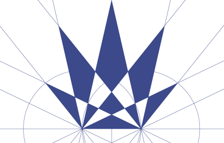
Figure 1: The corner points $r$, with $|r|\neq 0,1$ satisfy $U_{m}(r,\bar{r})=0$ when $m\equiv 0$ mod $7$. The two circles are $|r|=1$ and $|r+1|=1$.

8.3 Quadratic terms bilinear in $u$-, and $v$-derivatives

This section deals with the case $i=0$.

Proposition 14

If $H$ is a proper divisor of ${\mathcal{G}}^{0,1}_{1;m}[c{,}d](1,y)$ with $m(H)$ infinite then $H$ is a product of the following polynomials.

1. $y\in{\mathcal{H}}_{1}$, $m>0$, $c\neq 0$

2. $y^{n}\in{\mathcal{H}}_{n}$, $m\geq n$, $c=0$

3. $(y-r)\in{\mathcal{H}}_{2}$, $r\neq 0$, $m>1$

4. $(y-r)(y(1+r)+r)\in{\mathcal{H}}_{3}$, $m\equiv 1\mod 2$. When $(1+r)^{2n}=1$, $r\neq 0$, we also have $m\equiv 0\mod 2n$, $d=0$.

5. $(y-r)^{2}\in{\mathcal{H}}_{2n}$, $r\neq 0$, $n$ the smallest integer such that $(1+r)^{2n-1}=1$, $m\equiv 1\mod 2n-1$

6. $(y-r)^{2}(y(1+r)+r)^{2}\in{\mathcal{H}}_{2n+1}$, $n>1$ the smallest integer such that $(1+r)^{2n}=1$, $m\equiv 1\mod 2n$

7. $(y-r)(y(1+r)+r)(y-\bar{r})(y(1+\bar{r})+\bar{r})\in{\mathcal{H}}_{n}$, $n>3$ odd, $r=(\mu-\nu)/(\nu-1)$, $(\mu-1)(\nu-1)(\mu-\nu)(\mu\nu-1)\neq 0$, $n$ the smallest integer such that $\mu^{n}=\nu^{n}=1$, $m\equiv n\mod 2n$

8. $(y-r)(y-\bar{r})\in{\mathcal{H}}_{n}$, $n>2$ even, $r=(\mu-\nu)/(\nu-1)$, $(\mu-1)(\nu-1)(\mu-\nu)(\mu\nu-1)\neq 0$, $n$ the smallest integer such that $\mu^{n}=\nu^{n}=1$, $m\equiv 0\mod n$

9. $(y-r)(y(1+\bar{r})+\bar{r})\in{\mathcal{H}}_{n}$, $n>2$ even, $r=(\nu-\mu)/(\mu-1)$, $(\mu-\nu)(\mu\nu-1)\neq 0$, $n$ the smallest integer for which $\mu^{n}=\nu^{n}=-1$, $m\equiv n\mod 2n$

Unless stated otherwise, the coefficients of the linear part of the symmetries satisfy $c/d=r^{m}/((1+r)^{m}-1)$.

Proof: We are after the zeros of infinitely many

$${\mathcal{G}}^{0,1}_{1;m}[c{,}d](1,y)=c-c(1+y)^{m}+dy^{m}.$$

Take $c\neq 0$. Then $r\neq 0$ is a zero of precisely when

$$\frac{d}{c}=\frac{(1+r)^{m}-1}{r^{m}}.$$ (21)

When $m$ is odd $-r/(1+r)$ is a zero as well. The point $r=0$ is a zero for all $c,d,m$. It has multiplicity 1, except when $c=0$ where the multiplicity is $m$. One can show that the multiple zeros $r\neq 0$ of ${\mathcal{G}}^{0,1}_{1;m}[c{,}d]$ are the double zeros $\{r\neq 0:(1+r)^{m-1}=1\}$, with $c/d=r^{m-1}$. When $r$ is a double zero the only other double zero is $\bar{r}=-r/(1+r)$ when $m$ is odd.

Higher degree divisors are given by distinct non-zero $r,s\in\mathbb{C}$, with $r+rs+s\neq 0$ when $m$ is odd, such that the diophantine equation

$$U_{m}(r,s) = {\mathcal{G}}^{0,1}_{1,m}[r^{m},(1+r)^{m}-1](1,s)$$

$$= r^{m}-r^{m}(1+s)^{m}+s^{m}(1+r)^{m}-s^{m}=0$$

has infinitely many solutions $m$. The cases $r=-1$, $s=-1$ yield the primitive third roots of unity, as in Proposition 12, where $c=d=1$, which we excluded. Then, according to the the Skolem–Mahler–Lech theorem, at least one of the pairs

$$\frac{r}{s},\frac{r(1+s)}{s(1+r)}\quad\text{ or }\quad\frac{s}{r(1+s)},\frac{s}{r}(1+r)\quad\text{ or }\quad 1+r,1+s$$ (22)

consists of roots of unity. Suppose the first pair consist of roots of unity. Let $\mu=r/s$ and $\nu=r(1+s)/s/(1+r)$. Then $(\mu-1)(\nu-1)(\mu-\nu)\neq 0$, $\mu\nu\neq 1$ when $m$ odd, $r={\cal N}(\mu,\nu)$ and $s={\cal N}(1/\mu,1/\nu)=\bar{r}$ with

$${\cal N}(\mu,\nu)=\frac{\mu-\nu}{\nu-1}.$$

When $\mu\nu=1$ and $m$ even we have $\bar{r}=-r/(1+r)$. In terms of $\mu,\nu$ we get

$$U_{m}(r,s)=\left(\frac{\nu-\mu}{\mu(\nu-1)^{2}}\right)^{m}\left((1-\mu)^{m}(1-\nu^{m})-(1-\nu)^{m}(1-\mu^{m})\right),$$

which implies, using Theorem 7, that $\mu^{m}=\nu^{m}=1$. In bi-unit coordinates we have $r\in{\cal R}(\Phi_{2m},\Phi_{2m})$ such that ${|r+1|}\neq 1$ when $m$ odd.

Next, suppose that the second pair of (22) consists of roots of unity, $\mu=-r/s/(1+r)$, $\nu=-(1+s)r/s$. We have $(\mu-1)(\nu-1)(\mu-\nu)(\mu\nu-1)\neq 0$ when $r+rs+s\neq 0$, that is, when $m$ odd. When $r+rs+s=0$ and $m$ even we get $(1+r)^{m}=1$, which corresponds to $b=0$. Otherwise, $r={\cal K}(\mu,\nu)=(\nu-\mu)/(\mu-1)$ and $s=-\bar{r}/(1+\bar{r})$. In terms of $\mu,\nu$ we have

$$U_{m}(r,s)=\left(\frac{\nu-\mu}{\mu(\mu-1)(\nu-1)}\right)^{m}\left((1-\nu)^{m}(1+(-\mu)^{m})-(1-\mu)^{m}(1+(-\nu)^{m})\right)$$

When $m$ is odd Theorem 7 implies $\mu^{m}=\nu^{m}=1$, while for $m$ even Theorem 8 yields $\mu^{m}=\nu^{m}=-1$. The biunit coordinate description can be found as follows. Solve the simultaneous equations ${\cal K}(\mu,\nu)={\cal R}(\psi,\phi)$, ${\cal K}(1/\mu,1/\nu)={\cal R}(1/\psi,1/\phi)$ to find that $\mu=\psi^{2}/\phi^{2},\nu=\psi^{2}$. For odd $m$ we don’t find new values for $r$, but for $m$ even we get $r\in{\cal R}(\Phi_{4m}\setminus\Phi_{2m},\Phi_{2m})$ such that $|r+1|\neq 1$. Finally, suppose that the last pair of (22) consists of roots of unity. Then $\mu=1+r$ and $\nu=1+s$ satisfy equation (14). According to Theorem 7 we have $(1+r)^{m}=(1+s)^{m}=1$, that is, the second eigenvalue equals 0. $\square$

Actually, when $m$ is odd the two cases $i=-1,i=0$ are related. We have

$${\mathcal{G}}^{0,1}_{1;m}[c{,}d](1,r)={\mathcal{G}}^{-1,2}_{1;m}[c{,}d](1,-1-r).$$ (23)

Indeed, at odd order $m$ the zero $r=-1$ of ${\mathcal{G}}^{-1,2}_{1,m}$ translates into the zero $r=0$ of ${\mathcal{G}}^{0,1}_{1,m}$. Also the image of the unit circle $|z|=1$ under $f_{3}:r\rightarrow-1-r$ is the unit circle $|z+1|=1$, relating the double zeros of the two ${\mathcal{G}}$-functions. The symmetry $f_{2}:r\rightarrow 1/r$ is translated into $f_{4}=f_{3}\circ f_{2}\circ f_{3}:r\rightarrow-r/(1+r)$. And we note that set ${\cal R}(\Phi_{m},\Phi_{m})$ is invariant under the group of an-harmonic ratios, generated by $f_{2}$ and $f_{3}$, cf. [20]. Using the above, for odd $m$ one may obtain Propostion 14 from Proposition 13 and vise versa.

Summarizing this section, it implies that equations with homogeneous qua-dratic parts are approximately integrable when $n<4$. At any order $n\geq 4$ a finite number of new approximately integrable equations has been found.

9 Non-homogeneous quadratic parts

This section deals with equations whose quadratic part is not homogeneous, that is, $K^{1}=K^{i,1-i}_{1},K^{j,1-j}_{k}$ with $i\neq j$ when $k=1$. We provide the corresponding sets ${\mathcal{H}}^{2}_{n}$ of $2$-tuples. This time we do find conditions on the ratio $a/b$ for low orders $n<4$.

When $i=1$ the first part of the condition $H\in{\mathcal{H}}^{2}_{n}$, $H_{[1]}\in{\mathcal{H}}^{1}$ being a divisor of infinitely many ${\mathcal{G}}^{1,0}_{1;m}$, does not give conditions on $c/d$, see Proposition 12. In this case the ${\mathcal{H}}^{2}_{n}$ are obtained from the classification of $H_{[2]}\in{\mathcal{H}}^{1}$ dividing infinitely many ${\mathcal{G}}^{j,1-j}_{k;m}$, which was obtained in the previous section. A similar remark can be made when $(j,k)=(0,2)$. Due to equation (10) there are four cases left to consider, with $k=1$: $(i,j)=(-1,0)$; and with $k=2$: $(i,j)=(0,1)$, $(i,j)=(-1,2)$, $(i,j)=(-1,1)$.

There are certain divisors of infinitely many ${\mathcal{G}}_{m}[c{,}d]$-functions for any value of $c/d$. These will be called trivial divisors. Apart from the constant divisors we have

$$(1+y)\mid{\mathcal{G}}^{-1,2}_{1;2m+1}(1,y) y\mid{\mathcal{G}}^{-1,2}_{1;m}(1,y)$$

$$(x+1)\mid{\mathcal{G}}^{2,-1}_{2;2m+1}(x,1) x\mid{\mathcal{G}}^{1,0}_{2;m}(x,1)$$

We may take $H_{[1]}$ (or $H_{[2]}$) to be trivial. Then $H\in{\mathcal{H}}^{2}$ if $H_{[2]}$ ($H_{[1]}$) is one of the divisors of infinitely many ${\mathcal{G}}$-functions presented in the previous section. In the sequel we assume that neither $H_{[1]}$ nor $H_{[2]}$ is trivial. Also we will assume that $cd(c-d)\neq 0$.

Proposition 15

We list the non-trivial divisors $H$ of the 2-tuple ${\mathcal{G}}^{-1,2}_{1;m}[c{,}d](1,y)$, ${\mathcal{G}}^{1,0}_{2;m}[c{,}d](x,1)$ with $m(H)$ infinite. Firstly suppose $n$ is odd and $P(y)$ divides ${\mathcal{G}}^{-1,2}_{1;m}[c{,}d](1,y)$ with infinite $m(P)$ whose smallest element is $n$, cf. Proposition 13. Then $P(y),P(-1-x)\in{\mathcal{H}}_{n}$. Secondly, when $n$ is even we have:

1. $(y-r)(ry-1),x+1\in{\mathcal{H}}_{2}$, $r\in\Phi^{\prime}_{3}$, $m\equiv 2,4\mod 6$

2. $(y-r)^{2}(ry-1)^{2},x+1\in{\mathcal{H}}_{4}$, $r\in\Phi^{\prime}_{3}$, $m\equiv 4\mod 6$

3. $(y-r)(ry-1),\bar{r}x+\bar{r}+1\in{\mathcal{H}}_{n}$, $r=-\nu(\mu-1)/\mu/(\nu-1)$, $\mu\neq 1$, $n$ the lowest integer such that $\mu^{n}=-\nu^{n}=1$, $m\equiv n\mod 2n$.

The linear coefficients of the symmetries satisfy $c/d=(1+r^{m})/(1+r)^{m}$.

Proof: When the order of the equation $n$ is odd, no new conditions on the linear part are obtained since the relations (10) and (23) imply that

$${\mathcal{G}}^{-1,2}_{1;m}[c{,}d](1,-1-r)={\mathcal{G}}^{1,0}_{2;m}[c{,}d](r,1).$$

For even $n$, there should be $r\in\mathbb{C}$ with $s\neq 0$ such that

$${\mathcal{G}}^{-1,2}_{1;m}[c{,}d](1,r)={\mathcal{G}}^{1,0}_{2;m}[c{,}d](s,1)=0,$$

or, equivalently,

$$U_{m}(r,s)=s^{m}+(rs)^{m}+(1+r)^{m}-((1+r)(1+s))^{m}=0$$ (24)

for infinitely many $m$ including $n$. Then, using the Skolem-Mahler-Lech theorem, we may infer that either $rs(1+r)(1+s)=0$ or at least one of the pairs

$$r,1+s\qquad\frac{rs}{1+r},\frac{s}{(1+s)(1+r)},\qquad\frac{rs}{(1+r)(1+s)},\frac{s}{1+r}$$ (25)

consists of roots of unity. When $r(r+1)=0$ we have $c=d$ or $d=0$, which we excluded. When $s=-1$ we are left with the equation $U_{m}=(-1)^{m}+(-r)^{m}+(1+r)^{m}=0$. Applying the Skolem–Mahler–Lech theorem we see that both $r$ and $1+r$ are roots of unity and hence, that $r$ is a primitive third root of unity. One verifies that $U_{i+3k}=\left((-1)^{i}+(-r)^{i}+(1+r)^{i}\right)(-1)^{k}=0$ when $i$ equals 1 or 2. Also, if $-1$ is a zero of ${\mathcal{G}}^{1,0}_{2;m}[c{,}d]$, then $c/d=-(-1)^{m}$.

Suppose the first pair of (25) consists of roots of unity. Writing equation (24) in terms of $\mu=1+s$, $\nu=-r$, we get equation (16). Theorem 9 then implies $\mu^{m}=-\nu^{m}=1$, which corresponds to the case $a=0$, which we excluded. Suppose the second pair of (25) consists of roots of unity. Then $\mu=s/(1+s)/(1+r)$ and $\nu=-rs/(1+r)$ are roots of unity, and we get $r={\cal K}(u,v)=-\nu(\mu-1)/\mu/(\nu-1)$, $s=-(1+\bar{r})/\bar{r}$, and

$$U_{m}=\left(\frac{\mu-\nu}{(\mu-1)(\nu-1)\mu}\right)^{m}((1+(-\nu)^{m})(1-\mu)^{m}-(1-\mu^{m})(1-nu)^{m}).$$

When $m$ is even, Theorem 9 yields $\mu^{m}=-\nu^{m}=1$ or $\mu=1$. But, when $\mu=1$ we have $s=-(1+r)/r$ and $U_{m}=2(1+r)^{m}=0$ iff $r=-1$, which we excluded. Using ${\cal K}(1/\phi^{2},\psi^{2}/\phi^{2})={\cal R}(\psi,\phi)$ we may write $r\in{\cal R}(\Phi_{4m}\setminus\Phi_{2m},\Phi_{2m})$. When $n$ is even and $n$ is the lowest integer such that $\mu^{n}=-\nu^{n}=1$ we have $\mu$ is a primitive $n$-th root of unity or $\nu$ is a primitive $2n$-th root of unity and all solutions to $\mu^{n}=-\nu^{n}=1$ are given by $m\equiv n\mod 2n$.

The third pair of (25) is obtained from the second by $f_{2}:r\rightarrow 1/r$. Under this transformation we have ${\cal R}(\psi,\phi)\rightarrow{\cal R}(\psi^{-1},\phi\psi^{-1})$. Hence we get the solutions $r\in{\cal R}(\Phi_{4m}\setminus\Phi_{2m},\Phi_{4m}\setminus\Phi_{2m})$ and $s=-1-\bar{r}$. Or one can express $U_{m}=0$ in terms of $\mu=rs/(1+r)/(1+s)$, $\nu=-(1+r)/s$ to find these values. Another way of describing the last item would be: 3. $[(y-r)(ry-1),x+\bar{r}+1]\in{\mathcal{H}}_{n}$, $r=\mu(\nu-1)/(\mu-1)$, $\mu\neq 1$, $n$ the lowest integer such that $\mu^{n}=-\nu^{n}=1$, $m\equiv n\mod 2n$. $\square$

In the remaining cases the diophantine equation we obtain from the zeros of the ${\mathcal{G}}$-functions will be of the form

$$(1+aA^{m})(1+bB^{m})+cC^{m}=0.$$ (26)

Lemma 16

Suppose that the diophantine equation (26), with $ABC\neq 0$, has infinitely many solutions. Then $A$, $B$, and $C$ are roots of unity.

Proof: Using Corollary 6, three of the numbers $1,A,B,AB,C$ have a root of unity as a ratio and the same is true for the remaining two. Therefore at least one of the pairs $C,A$; $C,B$; $C/A,B$; $C/B,A$ consists of roots of unity. When $C$ and $A$ are roots of unity, their powers yield a finite number of values. Moreover, for the infinite number of solutions we have $(1+aA^{m})\neq 0$. Hence, for these infinite number of solutions $(1+bB^{m})$ has only finitely many values. This only happens when $B$ is a root of unity. The other cases lead to the same result, e.g. when $C/A$ and $B$ are roots of unity we divide the equation by $A^{m}$ and find that $A$ is a root of unity. $\square$

Suppose that the triple $\zeta,\eta,f(\zeta,\eta)$ consist of roots of unity. Then we can apply the algorithm of Smyth [4] to solve the equation $f(\zeta,\eta)^{-1}=f(\zeta^{-1},\eta^{-1})$ for roots of unity. In particular, a finite number of values will be obtained. We denote the set of all primitive $n$-th roots of unity by $\Phi^{\prime}_{n}$.

Proposition 17

We list the non-trivial divisors $H$ of the tuple ${\mathcal{G}}^{-1,2}_{1;m}[c{,}d](1,y)$, ${\mathcal{G}}^{0,1}_{1;m}(1,y)$ with $m(H)$ infinite.

1. $y^{2}+y+1,y+1\in{\mathcal{H}}_{2}$, $m\equiv 1,2\mod 3$, $c/d=-(-1)^{m}$

2. $(y^{2}+y+1)^{2},y+1\in{\mathcal{H}}_{4}$, $m\equiv 1\mod 3$, $c/d=-(-1)^{m}$

3. $(y-r^{2})(y-\bar{r}^{2})$, $(y-r+1)(y-\bar{r}+1)\in{\mathcal{H}}_{3}$, $r\in\Phi^{\prime}_{10}$, $m\equiv 1,3,7,9\mod 10$

4. $(y-r^{2})^{2}(y-\bar{r}^{2})^{2}$, $(y-r+1)^{2}(y-\bar{r}+1)^{2}\in{\mathcal{H}}_{11}$, $r\in\Phi^{\prime}_{10}$, $m\equiv 1\mod 10$

5. $(y-r)(y-\bar{r})$, $(y-r+1)(y-\bar{r}+1)\in{\mathcal{H}}_{5}$, $r\in\Phi^{\prime}_{12}$, $m\equiv 1,5,7,11\mod 12$

6. $(y-r)^{2}(y-\bar{r})^{2}$, $(y-r+1)^{2}(y-\bar{r}+1)^{2}\in{\mathcal{H}}_{13}$, $r\in\Phi^{\prime}_{12}$, $m\equiv 1\mod 12$

The linear coefficients of the symmetries satisfy $c/d=(r-1)^{m}/(r^{m}-1)$.

Proof: We have ${\mathcal{G}}^{-1,2}_{1;m}[c,d](1,r)={\mathcal{G}}^{0,1}_{1;m}[c,d](1,s)=0$ when

$$U_{m}(r,s)=(1+r^{m})(1-(1+s)^{m})+(s(1+r))^{m}=0.$$ (27)

We want to classify all $r,s\in\mathbb{C}$, with $rs(1+r)\neq 0$, such that equation (27) has infinitely many solutions. According to Lemma 16 we have $s=-1$, or $r,1+s,s(1+r)$ consists of roots of unity. When $s=-1$ we obtain that $r$ is a third root of unity and $U_{i+3k}=0$ iff $i=1,2$. When $x=r,y=1+s,f=s(1+r)$ consists of roots of unity, then $x,y$ are cyclotomic points on the curve

$$1+(xy-2(x-y))(xy-1)+(x-y)^{2}=0,$$

and can be found algorithmically. They are $x\in\Phi^{\prime}_{3}$, $y\in\Phi^{\prime}_{6}$; $y\in\Phi^{\prime}_{10}$, $x=y^{2}$ or $x=\bar{y}^{2}$; $y\in\Phi^{\prime}_{12}$, $x=y$ or $x=\bar{y}$. The first case only happens when $c=d$. In the second case we have $f=y^{4}$ or $f=y^{2}$ and we find $U_{i+10k}=0$ iff $i\in\{1,3,7,9\}$. Note that with $s=y-1$, ${|y|}=1$ we have $-s/(1+s)=\bar{s}$. The last case gives $f=y^{4}$ or $f=y^{3}$ and $U_{i+12k}=0$ iff $i\in\{1,5,7,11\}$.

The multiplicity of the zeros is obtained from Proposition 13 and 14. We have $r\in\Phi^{\prime}_{3}$ is a double zero of ${\mathcal{G}}^{-1,2}_{1;m}$ when $m\equiv 1$ mod $3$. When $y\in\Phi^{\prime}_{10}$ we have that both $r=y^{2}$ and $r=\bar{y}^{2}$ are in $\Phi^{\prime}_{5}$. They are double zeros of ${\mathcal{G}}^{-1,2}_{1;m}$ for $m\equiv 1$ mod $5$. Also, we have that $s=y-1$ and $\bar{s}$ are double zeros of ${\mathcal{G}}^{0,1}_{1;m}$ for $m\equiv 1$ mod $10$. A similar argument shows the multiplicity in the last item. $\square$

Proposition 18

We list the non-trivial divisors $H$ of the tuple ${\mathcal{G}}^{-1,2}_{1;m}[c{,}d](1,y)$, ${\mathcal{G}}^{2,-1}_{2;m}(x,1)$ with $m(H)$ infinite:

1. $(y-r)(y-\bar{r}),(x-r)(x-\bar{r})\in{\mathcal{H}}_{2}$, $r\in\Phi^{\prime}_{3}$, $m\equiv 1,2\mod 3$

2. $(y-r)^{2}(y-\bar{r})^{2},(x-r)^{2}(x-\bar{r})^{2}\in{\mathcal{H}}_{4}$, $r\in\Phi^{\prime}_{3}$, $m\equiv 1\mod 3$

3. $(y-r^{2})(y-\bar{r}^{2})$, $(x-r)(x-\bar{r})\in{\mathcal{H}}_{3}$, $r\in\Phi^{\prime}_{5}$, $m\equiv 1,3,7,9\mod 10$

4. $(y-r^{2})^{2}(y-\bar{r}^{2})^{2}$, $(x-r)^{2}(x-\bar{r})^{2}\in{\mathcal{H}}_{11}$, $r\in\Phi^{\prime}_{5}$, $m\equiv 1\mod 10$

5. $(y+r)(y+\bar{r})$, $(x-r)(x-\bar{r})\in{\mathcal{H}}_{4}$, $r\in\Phi^{\prime}_{12}$, $m\equiv 1,4,5,7,8,11\mod 12$

6. $(y+r)^{2}(y+\bar{r})^{2}$, $(x-r)^{2}(x-\bar{r})^{2}\in{\mathcal{H}}_{13}$, $r\in\Phi^{\prime}_{12}$, $m\equiv 1\mod 12$

The linear coefficients of the symmetries satisfy $c/d=(r+1)^{m}/(r^{m}+1)$.

Proof: We have ${\mathcal{G}}^{-1,2}_{1;m}[c,d](1,r)={\mathcal{G}}^{2,-1}_{2;m}[c,d](s,1)=0$ when

$$U_{m}(r,s)=(1+r^{m})(1+s^{m})-((1+s)(1+r))^{m}=0.$$ (28)

We want to classify all $r,s\in\mathbb{C}$, with $rs(s+1)(1+r)\neq 0$, such that equation (28) has infinitely many solutions. According to Lemma 16, the points $r$, $s$, and $(1+s)(1+r)$ are roots of unity. Hence $r,s$ are cyclotomic points on the curve

$$1+(rs+1)(rs+2(r+s))+(r+s)^{2}=0.$$

Smyths algorithm yields: $r,s\in\Phi^{\prime}_{3}$; $s\in\Phi^{\prime}_{5}$, $r=s^{2}$ or $r=\bar{s}^{2}$; $s\in\Phi^{\prime}_{12}$, $r=-s$ or $r=-\bar{s}$. Substitution these into the equation (28), we obtained, by performing some Groebner basis calculations, the solutions $m\equiv 1,2\mod 3$, $m\equiv 1,3,7,9\mod 10$, and $m\equiv 1,4,5,7,8,11\mod 12$ respectively. The multiplicities are determined using Proposition 13, and using relation (10). $\square$

Proposition 19

We list the non-trivial divisors $H$ of the tuple ${\mathcal{G}}^{0,1}_{1;m}[c{,}d](1,y)$, ${\mathcal{G}}^{1,0}_{2;m}(x,1)$ with $m(H)$ infinite:

1. $y+1-r,x+1-r\in{\mathcal{H}}_{2}$, $r=0$, $m>1$

2. $(y+1+r^{2})(y+1+\bar{r}^{2})$, $(x+1-r)(x+1-\bar{r})\in{\mathcal{H}}_{3}$, $r\in\Phi^{\prime}_{10}$, $m\equiv 1,3,7,9\mod 10$

3. $(y+1+r^{2})^{2}(y+1+\bar{r}^{2})^{2}$, $(x+1-r)^{2}(x+1-\bar{r})^{2}\in{\mathcal{H}}_{11}$, $r\in\Phi^{\prime}_{10}$, $m\equiv 1\mod 10$

4. $(y+1+r)$, $(x+1-r)\in{\mathcal{H}}_{2}$, $r\in\Phi^{\prime}_{12}$, $m\equiv 1,2,5,7,10,11\mod 12$

5. $(y+1+r)(y+1+\bar{r})$, $(x+1-r)(x+1-\bar{r})\in{\mathcal{H}}_{5}$, $r\in\Phi^{\prime}_{12}$, $m\equiv 1,5,7,11\mod 12$

6. $(y+1+r)^{2}(y+1+\bar{r})^{2}$, $(x+1-r)^{2}(x+1-\bar{r})^{2}\in{\mathcal{H}}_{13}$, $r\in\Phi^{\prime}_{12}$, $m\equiv 1\mod 12$

The linear coefficients of the symmetries satisfy $c/d=(r^{m}-1)/(r-1)^{m}$.

Proof: Similar to the above, ${\mathcal{G}}^{0,1}_{1;m}[c,d](1,r)={\mathcal{G}}^{1,0}_{2;m}[c,d](s,1)=0$ when

$$(1-(1+r)^{m})(1-(1+s)^{m})-(rs)^{m}=0.$$ (29)

We want to classify all $r,s\in\mathbb{C}$, with $rs\neq 0$, such that equation (29) has infinitely many solutions. If one of $r,s$ equals $-1$, the other is a third root of unity. When $r=s=-1$ we have $a/b=-(-1)^{m}$, otherwise $c=d$. Suppose that $(1+r)(1+s)\neq 0$. According to Lemma 16 $1+r$, $1+s$, and $sr$ are roots of unity. Then $x=1+r,y=1+s$ are cyclotomic points on the curve

$$1+(xy+1)(xy-2(x+y))+(x+y)^{2}=0.$$

They are: $x,y\in\Phi^{\prime}_{6}$; $y\in\Phi^{\prime}_{10}$, $x=-y^{2}$ or $x=-\bar{y}^{2}$; $y\in\Phi^{\prime}_{12}$, $x=-y$ or $x=-\bar{y}$. The first are zeros only when $c=d$ and the others yield the results. $\square$

10 Global classification of maximal degree divisors

Combining the results obtained in Propositions 12, 13, 14, 15, 17, 18, 19 we determine the set of all highest degree proper 6-tuples with infinite $m(H)$. This is equivalent to a global classification of approximately integrable two-component equations with a diagonal linear part, see section 6. Highest degree tuples are formed as follows. With $H\in{\mathcal{H}}_{n}$ and $F\in{\mathcal{H}}_{k}$ we have $HF\in{\mathcal{H}}_{l}$, where $l$ is the smallest number in $m(HF)=m(H)\cap m(F)$.

Clearly if $H$ divides ${\mathcal{G}}_{m}[c,d]$ then $H$ divides ${\mathcal{G}}_{m}[c/d,1]$. Also, if

$$H=[O(x_{1},x_{2}),P(x_{1},y_{1}),Q(y_{1},y_{2}),R(y_{1},y_{2}),S(x_{1},y_{1}),T(x_{1},x_{2})]$$

divides ${\mathcal{G}}_{m}[c,1]$ then, according to equation (10), the function ${\mathcal{G}}_{m}[1/c,1]$ admits the proper divisor

$$H^{\dagger}=[R(x_{1},x_{2}),S(y_{1},x_{1}),T(y_{1},y_{2}),O(y_{1},y_{2}),P(y_{1},x_{1}),Q(x_{1},x_{2})].$$

Thus we scale $d$ in ${\mathcal{G}}_{m}[c,d]$ to 1, and perform the classification up to inversion of $c$.

We also include tuples with zero components in the list. They correspond to equations that are not nonlinear injective, see section 5. For each $K^{0}$ in Table 1 we have determined the highest degree $r$-tuple $H$, with $m(H)$ infinite, which divides the $r$-tuple consisting of the non-zero components of its ${\mathcal{G}}_{n}$-tuple. The quadratic tuple $K^{1}$ has $r$ non-zero components $K^{1}={\mathcal{G}}_{n}/H$, unless complementary components of the ${\mathcal{G}}_{m}$-tuple vanish at infinitely $m\in m(H)$.

First we deal with ${\mathcal{H}}^{6}_{n\leq 5}$. Here we translate our symbolic results into differential language. For any $H\in{\mathcal{H}}_{n}$ of highest degree, which divides ${\mathcal{G}}_{n}[a,1]$, we determine $K^{1}$ from $\widehat{K}^{1}=[e,f,g,h,i,j]{\mathcal{G}}_{n}[a,1]/H$. In principal, the tuple $[e,f,g,h,i,j]$ may consist of proper polynomials, it is a common factor of $\widehat{K}^{1}$ and $\widehat{S^{1}}$. However, when writing down the differential equation, the $e,f,g,h,i,j$ will appear in it as constants, and any other constants will be absorbed by them. This organizes the quadratic part of the equations. At the same time it may remind the reader of the fact that the quadratic tuple of the equations can be multiplied by arbitrary proper tuples. We give each maximal degree tuple $H\in{\mathcal{H}}_{n}$ two indices, $H=H_{n.h}$, where $n$ is the order, and $h$ is a counter. We label the corresponding approximately integrable equation by $n.h$. And, we express the linear coefficients $c/d$ of the approximate symmetries in terms of integer sequences, or in its power sum solution if that displays well.

Secondly we give a general description of ${\mathcal{H}}^{6}_{n>5}$. Using this result one can, in principle, write down the corresponding approximate integrable systems at any particular order. Some Maple code has been provided at [15].

10.0 Zeroth order

According to Table 1 there are two special values of $a$ related to equations that are not nonlinear injective. We have the following 6-tuples in ${\mathcal{H}}_{0}$. At $a=0$

$$H_{0.1}=[0,1,1,1,0^{\ast},1].$$

Both the first and fifth component of the zeroth order ${\mathcal{G}}$-tuple vanishes. However, there exist higher order ${\mathcal{G}}$-tuple with zero first component, but no higher order ${\mathcal{G}}$-tuples with zero fifth component. This is denoted by the ^∗, which indicates that in the approximate integrable equation the term $K^{1,0}_{2}$ vanishes. The equation

$$\left(\begin{array}[]{c}u_{t}\\ v_{t}\end{array}\right)=\left(\begin{array}[]{c}eu^{2}+fuv+gv^{2}\\ v+hv^{2}+ju^{2}\end{array}\right)$$ 0.1

has approximate symmetries at order $m=1$, for all $c/d\in\mathbb{C}$, and at any order $m$, with $c=0$.

At $a=2$ we have

$$H_{0.2}=[1,1,0^{\ast},1,1,1].$$

The equation

$$\left(\begin{array}[]{c}u_{t}\\ v_{t}\end{array}\right)=\left(\begin{array}[]{c}2u+eu^{2}+fuv\\ v+hv^{2}+iuv+ju^{2}\end{array}\right)$$ 0.2

has approximate symmetries at any order $m\in\mathbb{N}$, for all $c,d\in\mathbb{C}$.

And, at generic values of $a$ we have

$$H_{0.3}=[1,1,1,1,1,1].$$

The equation, with $a(2a-1)(a-2)\neq 0$,

$$\left(\begin{array}[]{c}u_{t}\\ v_{t}\end{array}\right)=\left(\begin{array}[]{c}au+eu^{2}+fuv+gv^{2}\\ v+hv^{2}+iuv+ju^{2}\end{array}\right)$$ 0.3

has approximate symmetries at any order $m\in\mathbb{N}$, for all $c,d\in\mathbb{C}$.

10.1 First order

We have the following 6-tuples in ${\mathcal{H}}_{1}$. At $a=1$

$$H_{1.1}=[0,0^{\ast},0^{\ast},0^{\ast},0^{\ast},0^{\ast}].$$

The equation

$$\left(\begin{array}[]{c}u_{t}\\ v_{t}\end{array}\right)=\left(\begin{array}[]{c}u_{1}+eu^{2}\\ v_{1}\end{array}\right)$$ 1.1

has approximate symmetries at any order $m\in\mathbb{N}$, for $c=0$. Of course, when $e=0$ any $S\in{\mathfrak{g}}$ is a symmetry of this equation.

At generic values of $a$ we have

$$H_{1.2}=[0,y_{1},y_{1}+y_{2},0^{\ast},x_{1},x_{1}+x_{2}].$$

The equation, with $a\neq 1$,

$$\left(\begin{array}[]{c}u_{t}\\ v_{t}\end{array}\right)=\left(\begin{array}[]{c}au_{1}+eu^{2}+fuv+gv^{2}\\ v_{1}+iuv+ju^{2}\end{array}\right)$$ 1.2

has approximate symmetries at odd orders $m\equiv 1\mod 2$ for $c=0$. Again, when $e=0$ there are more approximate symmetries, namely at odd orders $m\equiv 1\mod 2$ for all $c,d\in\mathbb{C}$, see Remark 4.

10.2 Second order

At second order there is the tuple

$$H_{2}=[x_{1}x_{2},y_{1},1,y_{1}y_{2},x_{1},1]$$

which divides all higher ${\mathcal{G}}_{m}[c,d]$ for all $c,d\in\mathbb{C}$. The maximal degree divisors $H_{2.i}\in{\mathcal{H}}_{2}$ are $H_{2.i}=H_{2}T_{2.i}$ with

$$T_{2.1} = [0,y_{1},y_{1}^{2}+y_{2}^{2},1,x_{1}+2y_{1},(x_{1}+x_{2})^{2}]$$

$$T_{2.2} = [1,x_{1},y_{1}y_{2},1,y_{1},x_{1}x_{2}]$$

$$T_{2.3} = [1,x_{1}+y_{1},y_{1}^{2}+y_{1}y_{2}+y_{2}^{2},1,x_{1}+y_{1},x_{1}^{2}+x_{1}x_{2}+x_{2}^{2}]$$

$$T_{2.4} = [1,1,(ry_{2}-y_{1})(ry_{1}-y_{2}),1,1,1]$$

$$T_{2.5} = [1,rx_{1}-y_{1},1,1,1,1]$$

$$T_{2.6} = [1,1,(y_{1}+y_{2}-\iota y_{2})(2y_{1}+y_{2}+y_{2}\iota),1,2x_{1}+y_{1}+y_{1}\iota,1]$$

$$T_{2.7} = [1,2y_{1}-\iota x_{1}+2x_{1}+x_{1}\gamma,1,1,2x_{1}-y_{1}\gamma-\iota y_{1}+2y_{1},1],$$

where $\iota^{2}=-1,\gamma^{3}=3$.

The equation

$$\left(\begin{array}[]{c}u_{t}\\ v_{t}\end{array}\right)=\left(\begin{array}[]{c}eu^{2}+fuv+gv^{2}\\ v_{2}+hv^{2}+iuv+ju^{2}\end{array}\right)$$ 2.1

has approximate symmetries at orders $m\equiv 2\mod 4$ with $c=0$. The equation

$$\left(\begin{array}[]{c}u_{t}\\ v_{t}\end{array}\right)=\left(\begin{array}[]{c}u_{2}+eu^{2}+fuv+gv^{2}\\ v_{2}+hv^{2}+iuv+ju^{2}\end{array}\right)$$ 2.2

has approximate symmetries at all orders $m>1$ with $c=d=1$. The equation

$$\left(\begin{array}[]{c}u_{t}\\ v_{t}\end{array}\right)=\left(\begin{array}[]{c}-u_{2}+eu^{2}+fuv+gv^{2}\\ v_{2}+hv^{2}+iuv+ju^{2}\end{array}\right)$$ 2.3

has approximate symmetries at order $m\equiv 1,2\mod 3$, with $c/d=-(-1)^{m}$. The equation, with $(1+r^{2})(1+r)\neq 0$,

$$\left(\begin{array}[]{c}u_{t}\\ v_{t}\end{array}\right)=\left(\begin{array}[]{c}\frac{1+r^{2}}{(1+r)^{2}}u_{2}+eu^{2}+f(ruv_{1}-(1+r^{2})u_{1}v)+gv^{2}\\ v_{2}+hv^{2}+i(ru_{1}v-(1+r)^{2}uv_{1})+j(2ru_{2}u+(1+r)^{2}u_{1}^{2})\end{array}\right)$$ 2.4

has approximate symmetries at all orders $m>1$ with $c/d=(1+r^{m})/(1+r)^{m}$. The equation, with $r(r+2)\neq 0$,

$$\left(\begin{array}[]{c}u_{t}\\ v_{t}\end{array}\right)=\left(\begin{array}[]{c}\frac{r}{2+r}u_{2}+eu^{2}+fuv+g(rv_{1}^{2}-2vv_{2})\\ v_{2}+hv^{2}+i(u_{1}v+(2+r)uv_{1})+j(2uu_{2}+(2+r)u_{1}^{2})\end{array}\right)$$ 2.5

has approximate symmetries at all orders $m>1$ with $c/d=r^{m}/((1+r)^{m}-1)$.

The equation, with $\iota^{2}=-1$,

$$\left(\begin{array}[]{c}u_{t}\\ v_{t}\end{array}\right)=\left(\begin{array}[]{c}(-1+2\iota)u_{2}+eu^{2}+f(5u_{1}v+(3+\iota)uv_{1})+gv^{2}\\ v_{2}+hv^{2}+iuv+j(4uu_{2}+(1+\iota)u_{1}^{2})\end{array}\right)$$ 2.6

has approximate symmetries, with $c/d=-1+(-1)^{(m-2)/4}2^{m/2}\iota$, at order $m\equiv 2\mod 4$. The equation, with $\gamma^{2}=3$, $\iota^{2}=-1$,

$$\left(\begin{array}[]{c}u_{t}\\ v_{t}\end{array}\right)=\left(\begin{array}[]{c}\iota(2+\gamma)u_{2}+eu^{2}+fuv+g(4vv_{2}+(2+\gamma-\iota)v_{1}^{2})\\ v_{2}+hv^{2}+iuv+j(4uu_{2}+(2+\iota-\gamma)u_{1}^{2})\end{array}\right)$$ 2.7

has approximate symmetries at orders $m\equiv q\mod 12$, with $q\in\{1,2,5,7,10,11\}$. Define integers $P_{k}$ by $P_{1}=1$, $P_{2}=2$, and

$$P_{k}=\left\{\begin{array}[]{ll}P_{k-1}+P_{k-3}&k\equiv 1\mod 3\\ P_{k-1}+P_{k-2}&k\equiv 0,2\mod 3\end{array}\right..$$ (30)

When $q=2$ or $q=10$ the coefficients of the linear part of the approximate symmetries of equation 2.7 are given by

$$\frac{c}{d}=(-1)^{(m-q)/12}\iota(P_{3m/2-1}+P_{3m/2-2}\gamma),$$

or else by

$$\mp(-1)^{(m-q)/12}\frac{c}{d}=\left\{\begin{array}[]{ll}P_{(3m-5)/2}+P_{(3m-7)/2}\gamma&q=6\pm 5\\ P_{(3m+1)/2}+P_{(3m-1)/2}\gamma&q=6\pm 1\end{array}\right..$$ (31)

The sequence $\{P_{k}\}$ is quite interesting in itself, see [38, Sequence A140827]. It satisfies the 6-th order recurrence $P_{k}=4P_{k-3}-P_{k-6}$. And thus it consists of the three subsequences [38, Sequences A001075, A001353, A001835]. The first two of these subsequences are the denominators and numerators of convergents to $\sqrt{3}$, we have $P_{3n-1}^{2}-3P_{3n-2}^{2}=1$.

10.3 Third order

At third order the product

$$H_{3}=H_{2}[x_{1}+x_{2},1,y_{1}+y_{2},y_{1}+y_{2},1,x_{1}+x_{2}]$$

divides ${\mathcal{G}}_{m}[c,d]$ when $m$ odd, for all $c,d\in\mathbb{C}$. The maximal degree divisors $H_{3.i}\in{\mathcal{H}}_{3}$ are $H_{3.i}=H_{3}T_{3.i}$ where

$$T_{3.1} = [0,y_{1}^{2},y_{2}^{2}-y_{1}y_{2}+y_{1}^{2},1,x_{1}^{2}+3x_{1}y_{1}+3y_{1}^{2},(x_{1}+x_{2})^{2}]$$

$$T_{3.2} = [1,x_{1}(x_{1}+y_{1}),y_{1}y_{2},1,y_{1}(x_{1}+y_{1}),x_{1}x_{2}]$$

$$T_{3.3} = [1,1,(y_{1}-ry_{2})(y_{1}r-y_{2}),1,(rx_{1}+(1+r)y_{1})(x_{1}+(1+r)y_{1}),1]$$

$$T_{3.4} = [1,x_{1}^{2}+x_{1}y_{1}+(2-\phi)y_{1}^{2},y_{1}^{2}+\phi y_{1}y_{2}+y_{2}^{2},1,x_{1}^{2}+(2-\phi)(x_{1}y_{1}+y_{1}^{2}),$$

$$\hskip 204.85974ptx_{1}^{2}+(1-\phi)x_{1}x_{2}+x_{2}^{2}],$$

in which $\phi$ denotes the golden ratio or its conjugate, that is, $\phi(\phi-1)=1$. Note that both $H_{2.4}$ and $H_{2.5}^{\dagger}|_{-1-r}$ divide $H_{3.3}$.

The equation

$$\left(\begin{array}[]{c}u_{t}\\ v_{t}\end{array}\right)=\left(\begin{array}[]{c}eu^{2}+fuv+gv^{2}\\ v_{3}+hv^{2}+iuv+ju^{2}\end{array}\right)$$ 3.1

has approximate symmetries at orders $m\equiv 3\mod 6$ with $c=0$. The equation

$$\left(\begin{array}[]{c}u_{t}\\ v_{t}\end{array}\right)=\left(\begin{array}[]{c}u_{3}+eu^{2}+fuv+gv^{2}\\ v_{3}+hv^{2}+iuv+ju^{2}\end{array}\right)$$ 3.2

has approximate symmetries at odd orders with $c=d=1$. The equation, with $r^{3}\neq-1$,

$$\left(\begin{array}[]{c}u_{t}\\ v_{t}\end{array}\right)=\left(\begin{array}[]{c}\frac{1-r+r^{2}}{(1+r)^{2}}u_{3}+eu^{2}+f(ruv_{2}-(1-r+r^{2})(u_{2}v+u_{1}v_{1})\\ v_{3}+hv^{2}+iuv+j(2ruu_{2}+(1+r+r^{2})u_{1}^{2})\end{array}\right)$$ 3.3

has approximate symmetries at odd orders $m$ with $c/d=(1+r^{m})/(1+r)^{m}$. The equation, with $\phi(\phi-1)=1$,

$$\left(\begin{array}[]{c}u_{t}\\ v_{t}\end{array}\right)=\left(\begin{array}[]{c}-(2+3\phi)u_{3}+eu^{2}+fuv+gv^{2}\\ v_{3}+hv^{2}+iuv+ju^{2}\end{array}\right)$$ 3.4

has approximate symmetries at order $m\equiv q\mod 10$, $q\in\{1,3,7,9\}$, with

$$c/d=\left\{\begin{array}[]{ll}F_{m-2}+F_{m-1}\phi&q=5\pm 4\\ -F_{m}-F_{m+1}\phi&q=5\pm 2\\ \end{array}\right.,$$ (32)

where the $F_{k}$ are the Fibonacci numbers $F_{0}=0$, $F_{1}=1$, $F_{k}=F_{k-1}+F_{k-2}$ [38, Sequence A000045].

10.4 Fourth order

At order four the maximal degree divisors $H_{4.i}\in{\mathcal{H}}_{4}$ are $H_{4.i}=H_{2}T_{4.i}$ where

$$T_{4.1} = [0,y_{1}^{3},y_{1}^{4}+y_{2}^{4},1,(x_{1}+2y_{1})(x_{1}^{2}+2x_{1}y_{1}+2y_{1}^{2}),(x_{1}+x_{2})^{4}]$$

$$T_{4.2} = [1,x_{1}+y_{1},(y_{1}^{2}+y_{1}y_{2}+y_{2}^{2})^{2},1,x_{1}+y_{1},(x_{1}^{2}+x_{1}x_{2}+x_{2}^{2})^{2}]$$

$$T_{4.3} = [1,1,(y_{1}^{2}+2y_{1}y_{2}+2y_{2}^{2})(2y_{1}^{2}+2y_{1}y_{2}+y_{2}^{2}),1,1,1]$$

$$T_{4.4} = [1,(2y_{1}+(3-\gamma\iota)x_{1})^{2},1,1,1,1]$$

$$T_{4.5} = [1,x_{1}^{2}+2x_{1}y_{1}+2y_{1}^{2},1,1,1,1]$$

$$T_{4.6} = [1,y_{1}^{2}-2\iota x_{1}y_{1}-(1+\iota)x_{1}^{2},1,1,1,1]$$

$$T_{4.7} = [1,y_{1}^{2}+2(1-\iota\beta)x_{1}y_{1}-2\iota\beta x_{1}^{2},1,1,1,1]$$

$$T_{4.8} = [1,1,4y_{1}^{2}+(6-2\iota+2\iota\beta)y_{1}y_{2}+4y_{2}^{2},1,2x_{1}+(1-\iota+\iota\beta)y_{1},1]$$

$$T_{4.9} = [1,1,2y_{1}^{2}+(1-\iota-\iota\beta-2\beta)y_{1}y_{2}+2y_{2}^{2},1,2x_{1}+(1+\iota+\beta)y_{1},1]$$

$$T_{4.10} = [1,1,4y_{1}^{2}+(6-4\iota-3\iota\beta-\beta)y_{1}y_{2}+4y_{2}^{2},1,(1+\iota-\iota\beta)x_{1}+y_{1},1]$$

$$T_{4.11} = [1,1,y_{1}^{2}+y_{1}y_{2}\gamma+y_{2}^{2},1,1,x_{1}^{2}-x_{1}x_{2}\gamma+x_{2}^{2}],$$

with $\iota^{2}=-1,\beta^{2}=2,\gamma^{3}=3$.

The equation

$$\left(\begin{array}[]{c}u_{t}\\ v_{t}\end{array}\right)=\left(\begin{array}[]{c}eu^{2}+fuv+gv^{2}\\ v_{4}+h(4vv_{2}+3v_{1}^{2})+iuv+ju^{2}\end{array}\right)$$ 4.1

has approximate symmetries at orders $m\equiv 4\mod 8$ with $c=0$. The equation

$$\left(\begin{array}[]{c}u_{t}\\ v_{t}\end{array}\right)=\left(\begin{array}[]{c}-u_{4}+e(4u_{2}u+3u_{1}^{2})+f(uv_{2}+u_{1}v_{1}+2u_{2}v)+gv^{2}\\ v_{4}+h(4v_{2}v+3v_{1}^{2})+i(2uv_{2}+u_{1}v_{1}+u_{2}v)+ju^{2}\end{array}\right)$$ 4.2

has approximate symmetries at order $m\equiv 1\mod 3$ with $c/d=-(-1)^{m}$. The equation

$$\left(\begin{array}[]{c}u_{t}\\ v_{t}\end{array}\right)=\left(\begin{array}[]{c}\begin{split}-3u_{4}+e(4u_{2}u+3u_{1}^{2})+f(6u_{3}v+9u_{2}v_{1}+6u_{1}v_{2}\\ +2uv_{3})+gv^{2}\end{split}\\ \begin{split}v_{4}+h(4v_{2}v+3v_{1}^{2})+i(2u_{3}v+2u_{2}v_{1}+3u_{1}v_{2}+2uv_{3})\\ +j(4u_{4}u+4u_{1}u_{3}+3u_{2}^{2})\end{split}\end{array}\right)$$ 4.3

has approximate symmetries at order $m\equiv 0\mod 4$ with $c/d=1+(-1)^{m/4}2^{m/2}$. The equation, with $\zeta^{2}+\zeta+1=0$,

$$\left(\begin{array}[]{c}u_{t}\\ v_{t}\end{array}\right)=\left(\begin{array}[]{c}\begin{split}3(1+2\zeta)u_{4}+e(4uu_{2}+3u_{1}^{2})+f(6u_{1}v+(1-4\zeta)uv_{1})\\ +g(14v_{4}v+3(4-\zeta)(4v_{3}v_{1}+3v_{2}^{2}))\end{split}\\ \begin{split}v_{4}+h(4v_{2}v+3v_{1}^{2})+i(7u_{3}v+(2+3\zeta)(2u_{2}v_{1}+2uv_{3}\\ +3u_{1}v_{2}))+j(14u_{4}u+(2+3\zeta)(4u_{3}u_{1}+3u_{2}^{2}))\end{split}\end{array}\right)$$ 4.4

has approximate symmetries at order $m\equiv 1\mod 3$, with

$$\frac{c}{d}=\left\{\begin{array}[]{ll}(-3)^{(m-1)/2},&m\equiv 1\mod 6,\\ -(1+2\zeta)(-3)^{(m-2)/2},&m\equiv 4\mod 6.\end{array}\right.$$

The equation, with $\epsilon=\pm 1$,

$$\left(\begin{array}[]{c}u_{t}\\ v_{t}\end{array}\right)=\left(\begin{array}[]{c}\begin{split}\epsilon/5u_{4}+e(4uu_{2}+3u_{1}^{2})+f(2u_{1}v+(1-2\epsilon)uv_{1})\\ +g(4v_{3}v_{1}+3v_{2}^{2}+(1-5\epsilon)v_{4}v)\end{split}\\ \begin{split}v_{4}+h(4v_{2}v+3v_{1}^{2})+i(10(2u_{2}v_{1}+3u_{1}v_{2}+2uv_{3})\\ +(5-\epsilon)u_{3}v)+j(5(4u_{3}u_{1}+3u_{2}^{2})+(5-\epsilon)u_{4}u)\end{split}\end{array}\right)$$ 4.5

has approximate symmetries at order $m\equiv 0\mod 4$, with

$$\frac{c}{d}=\frac{\epsilon}{1-(-4)^{m/4}}.$$

The equation, with $\iota^{2}=-1$,

$$\left(\begin{array}[]{c}u_{t}\\ v_{t}\end{array}\right)=\left(\begin{array}[]{c}\begin{split}\iota/3u_{4}+e(4uu_{2}+3u_{1}^{2})+f(2u_{1}v+(1-2\iota)uv_{1})\\ +g(10vv_{4}+(1-3\iota)(4v_{1}v_{3}+3v_{2}^{2}))\end{split}\\ \begin{split}v_{4}+h(4v_{2}v+3v_{1}^{2})+i(5u_{3}v+3(3+\iota)(2u_{2}v_{1}+3u_{1}v_{2}\\ +2uv_{3}))+j(10u_{4}v+3(3+\iota)(3u_{2}^{2}+4u_{3}u_{1}))\end{split}\end{array}\right)$$ 4.6

has approximate symmetries at orders $m=4+k8$, $k\in\mathbb{N}$, with

$$\frac{c}{d}=\frac{(-1)^{k}2^{2k}\iota}{2A_{k+1}^{2}+1},$$

where the integers $A_{i}$ are the NSW numbers defined by $A_{0}=-1$ ,$A_{1}=1$, $A_{i}=6A_{i-1}-A_{n-2}$ [38, Sequence A002315]. The equation, with $\alpha^{2}=-2$

$$\left(\begin{array}[]{c}u_{t}\\ v_{t}\end{array}\right)=\left(\begin{array}[]{c}\begin{split}\alpha u_{4}+e(4uu_{2}+3u_{1}^{2})+f(2u_{1}v+(1-\alpha)uv_{1})\\ +g(2(4v_{1}v_{3}+3v_{2}^{2})+(2+\alpha)v_{4}v)\end{split}\\ \begin{split}v_{4}+h(4v_{2}v+3v_{1}^{2})+i((1-\alpha)u_{3}v+2(2u_{2}v_{1}+3u_{1}v_{2}\\ +2uv_{3}))+j(3u_{2}^{2}+4u_{3}u_{1}+(1-\alpha)u_{4}v)\end{split}\end{array}\right)$$ 4.7

has approximate symmetries at orders $m=4+k8$, $k\in\mathbb{N}$, with

$$\frac{c}{d}=\frac{(-1)^{k}2^{6k}\alpha}{B_{k+1}},$$

where the integers $B_{i}$ are defined by $B_{0}=-1$ ,$B_{1}=1$, $B_{i}=34B_{i-1}-B_{n-2}$ [38, Sequence A046176]. The equations, with $\iota^{2}=-1,\beta^{2}=2$,

$$\left(\begin{array}[]{c}u_{t}\\ v_{t}\end{array}\right)=\left(\begin{array}[]{c}\begin{split}(-1+2\iota(3+\beta))u_{4}+e(4uu_{2}+3u_{1}^{2})+f(6uv_{3}\\ +(9-\iota+2\beta)(2u_{1}v_{2}+3u_{2}v_{1}+2u_{3}v_{0}))\\ +g(12vv_{2}+(9+\beta+\iota)v_{1}^{2})\end{split}\\ \begin{split}v_{4}+h(4v_{2}v+3v_{1}^{2})+i(6u_{2}v+(3+5\iota-3\iota\beta-4\beta)u_{1}v_{1}\\ +2(1+3\iota-\iota\beta)uv_{2})+j(12uu_{4}\\ +(3+\iota-2\beta)(3u_{2}^{2}+4u_{3}u_{1}))\end{split}\end{array}\right)$$ 4.8

$$\left(\begin{array}[]{c}u_{t}\\ v_{t}\end{array}\right)=\left(\begin{array}[]{c}\begin{split}(-17+12\beta+2\iota(3-2\beta))u_{4}+e(4uu_{2}+3u_{1}^{2})+f(10uv_{3}\\ +(11-3\iota-6\beta-2\iota\beta)(2u_{1}v_{2}+3u_{2}v_{1}+2u_{3}v_{0}))\\ +g(20vv_{2}+(17-2\beta-\iota+\iota\beta)v_{1}^{2})\end{split}\\ \begin{split}v_{4}+h(4v_{2}v+3v_{1}^{2})+i(10u_{2}v+(13+\iota+7\beta+4\beta\iota)u_{1}v_{1}\\ +2(7-\iota+5\beta)uv_{2})+j(20uu_{4}\\ +(9+3\iota+2(3+\iota)\beta)(3u_{2}^{2}+4u_{3}u_{1}))\end{split}\end{array}\right)$$ 4.9

$$\left(\begin{array}[]{c}u_{t}\\ v_{t}\end{array}\right)=\left(\begin{array}[]{c}\begin{split}(17-12\beta+8\iota(3-2\beta))u_{4}+e(4uu_{2}+3u_{1}^{2})+f(12uv_{3}\\ -(3\beta+4\iota\beta-20+6\iota)(2u_{1}v_{2}+3u_{2}v_{1}+2u_{3}v_{0}))\\ +g(24vv_{2}+(22-3\beta+\iota\beta)v_{1}^{2})\end{split}\\ \begin{split}v_{4}+h(4v_{2}v+3v_{1}^{2})+i(2uv_{2}+(1+2\iota(\beta-1))u_{1}v_{1}\\ +(\iota-5+(4-\iota)\beta)u_{2}v)+j(24uu_{4}\\ +(4+6\iota+(3+4\iota)\beta)(3u_{2}^{2}+4u_{3}u_{1}))\end{split}\end{array}\right)$$ 4.10

have approximate symmetries at orders $m=4+k8$, $k\in\mathbb{N}$, with

$$\frac{c}{d} = -1+\iota(-1)^{k}2^{2k+1}(C_{m+1}+C_{m}\beta),$$

$$\frac{c}{d} = (-1+\iota(-1)^{k}2^{2k+1}(C_{m+1}+C_{m}\beta))(C_{2m+1}-C_{2m}\beta),$$

$$\frac{c}{d} = (1+\iota(-1)^{k}2^{6k+3}(C_{m+1}+C_{m}\beta))(C_{2m+1}-C_{2m}\beta),$$

respectively, where $C_{0}=0$, $C_{1}=1$, and $C_{2n}=C_{2n-1}+C_{2n-2}$, $C_{2n+1}=2C_{2n}-C_{2n-1}$. These integers, cf. [38, Sequence A002965], are the denominators and numerators of convergents to $\sqrt{2}$, we have

$$C_{n}^{2}-2C_{n-1}^{2}=\pm 1,\ \text{ when }\ n\equiv 1\pm 1\text{ mod }4.$$

The equation, with $\gamma^{2}=3$

$$\left(\begin{array}[]{c}u_{t}\\ v_{t}\end{array}\right)=\left(\begin{array}[]{c}\begin{split}(7+4\gamma)u_{4}+e(4uu_{2}+3u_{1}^{2})+f(2u_{1}v_{2}+3u_{2}v_{1}+2u_{3}v\\ +(2\gamma-3)uv_{3})+g(6vv_{2}+(6+\gamma)v_{1}^{2})\end{split}\\ \begin{split}v_{4}+h(4v_{2}v+3v_{1}^{2})+i((3+2\gamma)u_{3}v-2uv_{3}-3u_{1}v_{2}\\ -2u_{2}v_{1})+j(6uu_{2}+(6-\gamma)u_{1}^{2})\end{split}\end{array}\right)$$ 4.11

has approximate symmetries at order $m\equiv q\mod 12$, $q\in\{1,4,5,7,8,11\}$. When $q=6\pm 2$ the coefficients of the linear part of the approximate symmetries are given by

$$\frac{c}{d}=\mp(-1)^{(m-q)/12}(P_{3m/2-1}+P_{3m/2-2}\gamma),$$

where the integers $P_{k}$ are defined by the recursive formula (30). When $q$ is odd, $c/d$ is given by equation (31).

10.5 Fifth order

At order five the maximal degree divisors $H_{5.i}\in{\mathcal{H}}_{5}$ are $H_{5.i}=H_{5}T_{5.i}$ where

$$H_{5}=H_{3}[x_{1}^{2}+x_{1}x_{2}+x_{2}^{2},1,1,y_{1}^{2}+y_{1}y_{2}+y_{2}^{2},1,1]$$

and

$$T_{5.1} = [0,y_{1}^{4},y_{1}^{4}-y_{2}y_{1}^{3}+y_{1}^{2}y_{2}^{2}-y_{2}^{3}y_{1}+y_{2}^{4},1,x_{1}^{4}+5x_{1}^{3}y_{1}+10x_{1}^{2}y_{1}^{2}+10x_{1}y_{1}^{3}$$

$$\hskip 227.62204pt+5y_{1}^{4},(x_{1}+x_{2})^{4}]$$

$$T_{5.2} = [1,2y_{1}^{2}x_{1}^{2}+2x_{1}^{3}y_{1}+x_{1}^{4}+y_{1}^{3}x_{1},y_{1}^{3}y_{2}+y_{1}^{2}y_{2}^{2}+y_{2}^{3}y_{1},1,2y_{1}^{3}x_{1}+2y_{1}^{2}x_{1}^{2}$$

$$\hskip 156.49014pt+x_{1}^{3}y_{1}+y_{1}^{4},x_{1}^{3}x_{2}+x_{1}^{2}x_{2}^{2}+x_{1}x_{2}^{3}]$$

$$T_{5.3} = [1,1,ry_{1}^{2}-(1+r^{2})y_{1}y_{2}+ry_{2}^{2},1,rx_{1}^{2}+(1+r)^{2}(x_{1}y_{1}+y_{1}^{2}),1]$$

$$T_{5.4} = [1,1,(y_{1}^{2}+y_{2}^{2})^{2},1,(x_{1}^{2}+2x_{1}y_{1}+2y_{1}^{2})^{2},1]$$

$$T_{5.5} = [1,1,y_{1}^{4}+y_{2}^{4}+(2+\phi)(y_{1}^{3}y_{2}+y_{2}^{3}y_{1})+(4+\phi)y_{1}^{2}y_{2}^{2},1,x_{1}^{4}+(2-\phi)(y_{1}^{4}$$

$$\hskip 184.9429pt+x_{1}^{3}y_{1}+2y_{1}^{3}x_{1}+2y_{1}^{2}x_{1}^{2}),1]$$

$$T_{5.6} = [1,x_{1}^{2}+x_{1}y_{1}+(2-\gamma)y_{1}^{2},y_{1}^{2}+y_{1}y_{2}\gamma+y_{2}^{2},1,x_{1}^{2}+(2-\gamma)(x_{1}y_{1}+y_{1}^{2}),$$

$$\hskip 227.62204ptx_{1}^{2}-x_{1}x_{2}\gamma+x_{2}^{2}],$$

with $\gamma^{3}=3$ and $\phi(\phi-1)=1$. Note that $H_{5.3}=H_{5}T_{3.3}$ and, both $H_{2.7}$ and $H_{4.9}$ divide $H_{5.6}$.

The equation

$$\left(\begin{array}[]{c}u_{t}\\ v_{t}\end{array}\right)=\left(\begin{array}[]{c}eu^{2}+fuv+gv^{2}\\ v_{5}+hv^{2}+iuv+ju^{2}\end{array}\right)$$ 5.1

has approximate symmetries at orders $m\equiv 5,25\mod 30$ with $c=0$. The equation

$$\left(\begin{array}[]{c}u_{t}\\ v_{t}\end{array}\right)=\left(\begin{array}[]{c}u_{5}+eu^{2}+fuv+gv^{2}\\ v_{5}+hv^{2}+iuv+ju^{2}\end{array}\right)$$ 5.2

has approximate symmetries at orders $m\equiv 1,5\mod 6$ with $c=d=1$. The equation

$$\left(\begin{array}[]{c}u_{t}\\ v_{t}\end{array}\right)=\left(\begin{array}[]{c}\begin{split}\frac{1+r^{5}}{(1+r)^{5}}u_{5}+eu^{2}+f((r^{4}-r^{3}+r^{2}-r+1)(u_{1}v_{3}+2u_{2}v_{2}\\ +2u_{3}v_{1}+u_{4}v)-r(r^{2}+r+1)uv_{4})+g((1+r^{2})v_{1}^{2}\\ +2(r^{2}+r+1)vv_{2})\end{split}\\ \begin{split}v_{5}+hv^{2}+i((1+r)^{2}(uv_{2}+u_{1}v_{1})+(r^{2}+r+1)u_{2}v)\\ +j(2r(r^{2}+r+1)uu_{4}+2(r^{4}+3r^{3}+5r^{2}+3r+1)u_{1}u_{3}\\ +(r^{4}+5r^{3}+7r^{2}+5r+1)u_{2}^{2})\end{split}\end{array}\right)$$ 5.3

has approximate symmetries, with $c/d=(1+r^{m})/(1+r)^{m}$, at orders $m\equiv 1,5\mod 6$. The equation

$$\left(\begin{array}[]{c}u_{t}\\ v_{t}\end{array}\right)=\left(\begin{array}[]{c}-\frac{1}{4}u_{5}+eu^{2}+f(u_{4}v+2u_{3}v_{1}+2u_{2}v_{2}+u_{1}v_{3}+uv_{4})+gv^{2}\\ v_{5}+hv^{2}+iuv+j(2uu_{4}+6u_{1}u_{3}+5u_{2}^{2})\end{array}\right)$$ 5.4

has approximate symmetries, with $c/d=(-1)^{(m-1)/4}2^{(1-m)/2}$, at orders $m\equiv 1,5\mod 12$. The equation, with $\phi(\phi-1)=1$,

$$\left(\begin{array}[]{c}u_{t}\\ v_{t}\end{array}\right)=\left(\begin{array}[]{c}\begin{split}-(4+5\phi)u_{5}+eu^{2}+f((4-\phi)uv_{4}+11(u_{1}v_{3}+2u_{2}v_{2}\\ +2u_{3}v_{1}+u_{4}v))+gv^{2}\end{split}\\ v_{5}+hv^{2}+iuv+j(2\phi uu_{4}-2u_{1}u_{3}+(2\phi-1)u_{2}^{2})\end{array}\right)$$ 5.5

has approximate symmetries at orders $m\equiv 5,25\mod 30$, with $c/d=-(1+F_{m-1}+F_{m}\phi)$, where $F_{m}$ denotes the $m$-th Fibonacci number. And, the equation, with $\gamma^{2}=3$,

$$\left(\begin{array}[]{c}u_{t}\\ v_{t}\end{array}\right)=\left(\begin{array}[]{c}\begin{split}(26+15\gamma)u_{5}+eu^{2}+f(u_{2}v+u_{1}v_{1}+(\gamma-1)uv_{2})\\ +g(4vv_{2}+(3+\gamma)v_{1}^{2})\end{split}\\ \begin{split}v_{5}+hv^{2}+i(u_{1}v_{1}+uv_{2}-(1+\gamma)u_{2}v)\\ +j(4uu_{2}+(3-\gamma)u_{1}^{2}\end{split}\end{array}\right)$$ 5.6

has approximate symmetries at orders $m\equiv 1,5\mod 6$, with $c/d$ given by equation (31).

10.6 Higher order

Define

$$H_{7}=H_{5}[x_{1}^{2}+x_{1}x_{2}+x_{2}^{2},1,1,y_{1}^{2}+y_{1}y_{2}+y_{2}^{2},1,1],$$

and, for convenience, $H_{2n}=H_{2}$, $H_{2n+1}=H_{k}$, where $n\equiv k$ mod $6$ and $k\in\{3,5,7\}$. We first list the divisors that have similar structure at infinitely many higher orders. After that we consider the exceptional cases.

The case $a=0$

1. The tuple ${\mathcal{G}}_{n}[0,1]$ has the following divisor in ${\mathcal{H}}^{6}_{n}$

   $$[0,y_{1}^{n},y_{1}^{n}+y_{2}^{n},X,y_{1}^{n}-(x_{1}+y_{1})^{n},(x_{1}+x_{2})^{n}].$$ (33)

   where $X$ is the fourth component of $H_{n}$. It divides ${\mathcal{G}}_{m}[0,1]$ when

   $$m\equiv\left\{\begin{array}[]{ll}n\text{ mod }2n,&n\text{ even, or }n\equiv 3\text{ mod }6,\\ n\text{ mod }6n,&n\equiv 1\text{ mod }6,\\ n,5n\text{ mod }6n,&n\equiv 5\text{ mod }6.\end{array}\right.$$

The case $n$ is even

Let $n>2$ be even. We have the following divisors in ${\mathcal{H}}_{n}^{6}$.

1. For any primitive ($n-1$)-st root of unity $r$

   $$H_{2}[1,1,(y_{1}-ry_{2})^{2}(ry_{1}-y_{2})^{2},1,1,1]$$ (34)

   divides ${\mathcal{G}}_{m}[(1+r)^{1-m},1]$ when $m\equiv 1$ mod $n-1$.

2. Let one of $\mu,\nu$ be an $n$-th root of unity, and the other a primitive $n$-th root of unity, such that $(\mu-1)(\nu-1)(\mu-\nu)(\mu\nu-1)\neq 0$. Then, with $r=\nu(\mu-1)/(\nu-1)$

   $$H_{2}[1,1,(y_{1}-ry_{2})(ry_{1}-y_{2})(y_{1}-\bar{r}y_{2})(\bar{r}y_{1}-y_{2}),1,1,1]$$

   divides ${\mathcal{G}}_{m}[1+r^{m},(1+r)^{m}]$ when $m\equiv 0$ mod $n$.

3. For any primitive ($n-1$)-st root of unity $r$

   $$H_{2}[1,(y_{1}-(r-1)x_{1})^{2},1,1,1,1]$$ (35)

   divides ${\mathcal{G}}_{m}[(r-1)^{m-1},1]$ when $m\equiv 1$ mod $n-1$.

4. Let one of $\mu,\nu$ be a primitive $n$-th root of unity, and the other a $n$-th root of unity, such that $(\mu-1)(\nu-1)(\mu-\nu)(\mu\nu-1)\neq 0$. Then, with $r=(\mu-\nu)/(\nu-1)$

   $$H_{2}[1,(y_{1}-rx_{1})(y_{1}-\bar{r}x_{1}),1,1,1,1]$$

   divides ${\mathcal{G}}_{m}[r^{m},(1+r)^{m}-1]$ when $m\equiv 0$ mod $n$.

5. Let one of $\mu,\nu$ be a primitive $2n$-th root of unity, and the other a primitive $2n$-th root of unity which is not a $n$-th root of unity, such that $(\mu-\nu)(\mu\nu-1)\neq 0$. Then, with $r=(\nu-\mu)/(\mu-1)$

   $$H_{2}[1,(y_{1}-rx_{1})(y_{1}(1+\bar{r})+\bar{r}x_{1}),1,1,1,1]$$

   divides ${\mathcal{G}}_{m}[r^{m},(1+r)^{m}-1]$ when $m\equiv n$ mod $2n$.

6. Let either $\mu$ be a primitive $n$-th root of unity and $\nu$ be a $2n$-th root of unity which is not a $n$-th root of unity, or let $\mu\neq 1$ be a $n$-th root of unity and $\nu$ a primitive $2n$-th root of unity. Then, with $r=-\nu(\mu-1)/(\nu-1)/\mu$

   $$H_{2}[1,1,(y_{2}-ry_{1})(ry_{2}-y_{1}),1,1,\bar{r}x_{1}+(1+\bar{r})y_{1},1]$$

   divides ${\mathcal{G}}_{m}[1+r^{m},(1+r)^{m}]$ when $m\equiv n$ mod $2n$.

The case $n$ is odd

Let $n>3$ be odd. We have the following divisors in ${\mathcal{H}}_{n}^{6}$.

1. For any primitive ($n-1$)-st root of unity $r$ define

   $$Q_{n}(r)=[1,1,(y_{1}-ry_{2})^{2}(ry_{1}-y_{2})^{2},1,(x_{1}+(1+r)y_{1})^{2}(rx_{1}+(1+r)y_{1})^{2},1].$$

   The tuple $H_{n}Q_{n}(r)$ divides ${\mathcal{G}}_{m}[(1+r)^{1-m},1]$ when

   $$m\equiv\left\{\begin{array}[]{ll}1\text{ mod }n-1,&n\equiv 1,3\text{ mod }6,\\ 1,n\text{ mod }3(n-1),&n\equiv 5\text{ mod }6.\end{array}\right.$$

2. Let one of $\mu,\nu$ be a $n$-th root of unity, and the other a primitive $n$-th root of unity, such that $(\mu-1)(\nu-1)(\mu-\nu)(\mu\nu-1)\neq 0$. Then, with $r=\nu(\mu-1)/(\nu-1)$ we define

   $$\begin{split}W_{n}(r)=[1,1,(y_{1}-ry_{2})(ry_{1}-y_{2})(y_{1}-\bar{r}y_{2})(\bar{r}y_{1}-y_{2}),1,(x_{1}+(1+\bar{r})y_{1})\\ \hskip 48.36967pt(\bar{r}x_{1}+(1+\bar{r})y_{1})(x_{1}+(1+\bar{r})y_{1})(\bar{r}x_{1}+(1+\bar{r})y_{1}),1].\end{split}$$

   The tuple $H_{n}W_{n}(r)$ divides ${\mathcal{G}}_{m}[1+r^{m},(1+r)^{m}]$ when

   $$m\equiv\left\{\begin{array}[]{ll}n\text{ mod }6n,&n\equiv 1\text{ mod }6,\\ n\text{ mod }2n,&n\equiv 3\text{ mod }6,\\ n,5n\text{ mod }6n,&n\equiv 5\text{ mod }6.\end{array}\right.$$

We also get new highest degree divisors in ${\mathcal{H}}_{n}^{6}$, with $n$ odd, from primitive $p$-th roots of unity with $p<n$. This happens when $n\equiv 1$ mod $p$ (or $n\equiv 0$ mod $p$) and $n\equiv k$ mod $6$ with $k\in\{3,5,7\}$, such that there is no $1<q<n$ with $q\equiv 1$ mod $p$ (or $q\equiv 0$ mod $p$), and $q\equiv l$ mod $6$ with $l\in\{3,5,7\}$ and $l\geq k$. For example, the tuple $T_{5.4}$ divides a ${\mathcal{G}}_{m}$ at $m\equiv 1$ mod $4$. The tuple $H_{5.4}=H_{5}T_{5.4}$ divides a ${\mathcal{G}}_{m}$ at $m\equiv 1,5$ mod $12$, see equation 5.4. We have $13\equiv 1$ mod $4$ and $13\equiv 7$ mod $6$. There is no $1<q<13$ such that $q\equiv 1$ mod $4$ and $q\equiv l$ mod $6$, with $l\in{3,5,7}$ and $l\geq 7$. Thus, the tuple $H_{7}T_{5.4}\in{\mathcal{H}}_{13}$ divides a ${\mathcal{G}}_{m}$ at $m\equiv 1$ mod $12$. We have $9\equiv 1$ mod $4$ and $9\equiv 3$ mod $6$, but there is $q=5$ such that $q\equiv 1$ mod $4$ and $q\equiv 5$ mod $6$, and $5\geq 3$. Therefore the tuple $H_{3}T_{5.4}$ is not in ${\mathcal{H}}_{9}$. It is in ${\mathcal{H}}_{5}$ but it does not have maximal degree.

Also, we may have $p$ odd. If the tuple (34) divides ${\mathcal{G}}_{m}[(1+r)^{1-m},1]$ when $m\equiv 1$ mod $p$, then, according to Proposition 15, $Q^{p+1}_{(r)}$ divides ${\mathcal{G}}_{2p+1}[(1+r)^{2p},1]$. This always give us a new highest degree tuple in ${\mathcal{H}}_{2p+1}$. On the other hand, from case iii one can conclude, using Propositions 14 and 15 and inverting $a\rightarrow 1/a$, that $Q_{p+1}(-r)$ divides ${\mathcal{G}}_{2p+1}[(1+r)^{2p},1]$. This we knew already, since when $r$ is a primitive $p$-th root of unity, with $p$ odd, then $-r$ is a $2p$-th root of unity, cf. case viii.

In general one can show the following.

• Suppose $n\equiv 0$ mod $p$ and $n\equiv k$ mod $6$ with $k\in\{3,5,7\}$, such that there is no $q<n$ with $q\equiv 0$ mod $p$, and $q\equiv l$ mod $6$ with $l\in\{3,5,7\}$ and $l\geq k$. Then $p$ is odd. And,

  $$n=\left\{\begin{array}[]{ll}p,&p\equiv 1,3\text{ mod }6,\\ p,5p&p\equiv 5\text{ mod }6.\end{array}\right.$$ (36)

• Suppose $n\equiv 1$ mod $p$ and $n\equiv k$ mod $6$ with $k\in\{3,5,7\}$, such that there is no $q<n$ with $q\equiv 1$ mod $p$, and $q\equiv l$ mod $6$ with $l\in\{3,5,7\}$ and $l\geq k$. Then

  $$n=\left\{\begin{array}[]{ll}p+1&p\equiv 0\text{ mod }6,\\ p+1,2p+1,4p+1,6p+1&p\equiv 1\text{ mod }6,\\ p+1,2p+1,3p+1&p\equiv 2\text{ mod }6,\\ p+1,2p+1&p\equiv 3\text{ mod }6,\\ p+1,3p+1&p\equiv 4\text{ mod }6,\\ p+1,2p+1,6p+1&p\equiv 5\text{ mod }6.\end{array}\right.$$ (37)

We can now describe all highest degree divisors at odd order $n$, involving the tuples $Q,W$. For odd $n$ there are the cases viii and ix described above. They corresponds to the cases $n=p+1$ in (37), and $n=p$ in (36), respectively. Furthermore we have:

1. If $n=5p$ and $p\equiv 5$ mod $6$, then $H_{n}W_{p}(r)$ divides ${\mathcal{G}}_{m}[1+r^{m},(1+r)^{m}]$ when $m\equiv 5p$ mod $6p$.

2. If $n\equiv 1,3$ mod $6$ and equation (37) holds for certain $p$, then $H_{n}Q_{p}(r)$ divides ${\mathcal{G}}_{m}[1+r^{m},(1+r)^{m}]$ when $m\equiv 1$ mod $n-1$.

3. Let $n\equiv 5$ mod $6$. If $n=2p+1$, $p\equiv 5$ mod $6$ then $H_{n}Q_{p}(r)$ divides ${\mathcal{G}}_{m}[1+r^{m},(1+r)^{m}]$ when $m\equiv 1,n$ mod $3(n-1)$. And if $n=2p+1$, $p\equiv 2$ mod $6$, or $n=4p+1$, $p\equiv 1$ mod $6$, then $H_{n}Q_{p}(r)$ divides ${\mathcal{G}}_{m}[1+r^{m},(1+r)^{m}]$ when $m\equiv 1,n$ mod $3(n-1)/2$.

Exceptional highest degree divisors, $n\geq 7$

1. The tuple ${\mathcal{G}}_{7}[1,1]\in{\mathcal{H}}_{7}$ divides ${\mathcal{G}}_{m}[c,d]$ with $m\equiv 1$ mod $6$ and $c=d=1$.

2. The tuple $H_{7}T_{3.3}\in{\mathcal{H}}_{7}$ divides ${\mathcal{G}}_{m}[1+r^{m},(1+r)^{m}]$ with $m\equiv 1$ mod $6$.

3. The tuple $H_{7}T_{3.4}\in{\mathcal{H}}_{7}$ divides ${\mathcal{G}}_{m}[c,d]$ with $m\equiv 1,7,13,19$ mod $30$ and $c,d$ given by equation 32.

4. The tuple $H_{7}T_{5.6}\in{\mathcal{H}}_{7}$ divides ${\mathcal{G}}_{m}[c,d]$ with $m\equiv 1$ mod $6$ and $c,d$ given by equation 31.

5. Define

   $$Z=[1,(x_{1}^{2}+x_{1}y_{1}+(1+\phi)y_{1}^{2})^{2},(y_{1}^{2}+(1-\phi)y_{1}y_{2}+y_{2}^{2})^{2},1,\$$

   $$(x_{1}^{2}+(1+\phi)(x_{1}y_{1}+y_{1}^{2}))^{2},(x_{1}^{2}+\phi x_{1}x_{2}+x_{2}^{2})^{2}].$$

   Then $H_{5}Z\in{\mathcal{H}}_{11}$ divides ${\mathcal{G}}_{m}[c,d]$ with $m\equiv 1,11$ mod $30$ and $c/d$ given by equation (32). And $H_{7}Z\in{\mathcal{H}}_{31}$ divides ${\mathcal{G}}_{m}[c,d]$ with $m\equiv 1$ mod $30$.

6. The tuple

   $$H_{7}[1,(x_{1}^{2}+x_{1}y_{1}+(2-\gamma)y_{1}^{2})^{2},(y_{1}^{2}+\gamma y_{1}y_{2}+y_{2}^{2})^{2},1,\$$

   $$(x_{1}^{2}+(2-\gamma)(x_{1}y_{1}+y_{1}^{2}))^{2},(x_{1}^{2}-\gamma x_{1}x_{2}+x_{2}^{2})^{2}]\in{\mathcal{H}}_{13}$$

   divides ${\mathcal{G}}_{m}[c,d]$ with $m\equiv 1$ mod $12$ and $c/d$ given by equation (31).

11 Concluding remarks

In the formal symmetry approach [25], as well as in the computer-assisted schemes [9, 40], not knowing the ratios of eigenvalues strongly complicates the classification of integrable equations. There the ratios are obtained, if possible at all, at the very last stage of the calculations. We hope that the a priori knowledge provided in this article will be an impetus to complete the classification.

Usually, in classification programs one considers homogeneous equations. A 2-component equation $(u_{t},v_{t})=K$ is homogeneous of weighting $\lambda$ if $K$ is an eigenvector of ${\mathcal{L}}(\sigma_{x}+\lambda_{1}\sigma_{u}+\lambda_{2}\sigma_{v})$, where $\sigma_{x}=(xu_{1},xv_{1})$ counts the number of derivatives. We have compactly provided a list of nonhomogeneous equations. A complete list of homogeneous equations can be obtained from our list by multiplying the symbolic quadratic parts with appropriate tuples of polynomials. And Lemma 3 can be used to determine all symmetries of those equations.

A classification of second order integrable 2-component evolution equations has been given in [35]. The lemmas 6.3, 6.4, 6.5, and 6.6, proved in there, are special cases ($n=2$) of Proposition 15, 18, 19, and 17, respectively. In [35] the full analysis of higher order symmetry conditions was carried out completely. From this it follows that all second order integrable equations with quadratic parts are derived from equations 2.3, 2.4, and 2.5. Note that the authors of [35] excluded equations of type 2.1 and 2.2.

A classification of third order 2-component evolution equations with weighting $(2,2)$ and symmetries of order 5, 7, or 9, is given in [9]. Of the five equations listed [9, Theorem 3.3], two are nonlinear injective and have diagonalizable linear part:

$$\left(\begin{array}[]{c}u_{t}\\ v_{t}\end{array}\right)=\left(\begin{array}[]{c}u_{3}+uu_{1}+vv_{1}\\ -2v_{3}-uv_{1}\end{array}\right)$$ (38)

and

$$\left(\begin{array}[]{c}u_{t}\\ v_{t}\end{array}\right)=\left(\begin{array}[]{c}4u_{3}+3v_{3}+4uu_{1}+vu_{1}+2uv_{1}\\ 3u_{3}+v_{3}-2vv_{1}-4vu_{1}-2uv_{1}\end{array}\right).$$ (39)

When put in Jordan form the ratio of the coefficients of the linear part of equation (39) becomes $a/b=-3\phi-2$, where $\phi$ is the golden ratio. Our diophantine approach perfectly explains the ’unusual’ symmetry pattern. We remark that the conjugate of $\phi$ gives rise to another equation with $a/b=-3(1-\phi)-2=1/(-3\phi-2)$, which can be obtained by interchanging $u$ and $v$. A similar remark holds for all equations derived from the ’symmetric’ Propositions 18 and 19. For example, by interchanging $u$ and $v$ in equation 4.11 we get an equation with $a/b=1/(7+4\gamma)=7-4\gamma$.

According to [9, Theorem 3.3] we have the following. A non-decouplable fifth order two component equation in the KDV weighting, possessing a generalized symmetry of order 7 can be reduced by a linear change of variables to a symmetry of lower order equations, or to the Zhou-Jiang-Jiang equation,

$$\left(\begin{array}[]{c}u_{t}\\ v_{t}\end{array}\right)=\left(\begin{array}[]{c}\begin{split}u_{5}-5(2uu_{3}+5u_{1}u_{2})+15(2vv_{3}+3v_{1}v_{2})+20u_{1}u^{2}\\ -30(u_{1}v^{2}+2uvv_{1})\end{split}\\ \begin{split}-9v_{5}+5(2u_{3}v+7u_{2}v_{1}+9u_{1}v_{2}+6uv_{3})-10(2uu_{1}v\\ +2u^{2}v_{1}+3v^{2}v_{1})\end{split}\end{array}\right).$$

However, since the ratio of coefficients of the linear part $a/b=-1/9$ does not appear in our list, this equation has an approximate symmetry at lower order. In fact, the equation has a genuine symmetry at third order. The Zhou-Jiang-Jiang equation is in the hierarchy of the Drinfel d-Sokolov type [7] equation

$$\left(\begin{array}[]{c}u_{t}\\ v_{t}\end{array}\right)=\left(\begin{array}[]{c}-3vv_{1}\\ v_{3}-u_{1}v-2uv_{1}\end{array}\right),$$ (40)

which is linearly equivalent to a third order equation that appears in the same paper [9, Equation (17)], cf. [40, Sections 3.2.1, 4.2.6]. The special value of the ratio $a/b=-1/2$ in equation (38) also does not appear in our list and is due to higher grading constraints. At the end of [24] two fifth order systems are given with ratios $(9-5\sqrt{3})(9+5\sqrt{3})^{-1}=26-15\sqrt{3}$ and $-1/9$. The first system derives from equation 5.6 and the latter from equation 5.3, with $r$ a primitive $6$-th root of unity.

We conclude with a more philosophical remark and some ideas on future research. The concept of generalized symmetry really is about local symmetry. The (inverse) Gel’fand-Dikiĭ transformation translates polynomials in the symbols $x,y$ into local differential functions, that is expressions in $u,v$ and their derivatives. A question arises: can we also translate rational functions in the symbols $x,y$? The answer is yes. One could think of non-local variables $u_{i},v_{i}$ with $0>i\in\mathbb{Z}$. Here a negative index indicates integration and $D_{x}$ would be such that $D_{x}(u_{i-1})=u_{i}$ for all $i$. We can expand rational functions in Taylor-series, which are transformed into non-local differential sums. For example, consider the rational function $\widehat{F}=1/(x_{1}+x_{2})$. Its symmetric Taylor-series is

$$\widehat{F}=\frac{1}{2}\sum_{k=0}^{\infty}(-1)^{k}(\frac{x_{1}^{k}}{x_{2}^{k+1}}+\frac{x_{2}^{k}}{x_{1}^{k+1}})$$

which is transformed into the non-local object

$$F=\sum_{k=0}^{\infty}(-1)^{k}u_{k}u_{-k-1},$$

and we have $D_{x}F=u^{2}$. In this non-local setting every equation has a symmetry at any order. For example, the equation, with $a\neq 1$,

$$\left(\begin{array}[]{c}u_{t}\\ v_{t}\end{array}\right)=\left(\begin{array}[]{c}au_{1}+(1-a)uv\\ v_{1}+(1-a)uv\end{array}\right),$$

and its approximate symmetries (but the ones in ${\mathcal{A}}^{2,0}\otimes{\mathcal{A}}^{0,2}$), are in the approximate hierarchy of the zeroth order non-local equation

$$\left(\begin{array}[]{c}u_{t}\\ v_{t}\end{array}\right)=\left(\begin{array}[]{c}u+uv_{-1}\\ v-u_{-1}v\end{array}\right).$$

Still, there would be a quest for equations, or symmetries, that are in certain sense close to local.

Since the pioneering work of Sanders and Wang [34], apart from extending the result to equations with more more components [3, 35, 12], the symbolic method has been further developed in order to classify non-commutative [30], non-evolutionary [21, 23, 28], non-local [21, 22], and multi-dimensional equations [41]. In classifying non-local equations the concept of quasi-locality, introduced in [26] is the key idea. Only certain types of non-localities are allowed by considering different extensions of the ring of differential polynomials. ‘Nnon-evolutionary’ equations are treated as evolution equations with possible non-localities. For example, a Boussinesq type scalar equation

$$u_{tt}=K(u,u_{x},u_{xx}\ldots,u_{t},u_{xt},\ldots$$

can be represented as a two-component evolution equation,

$$\left(\begin{array}[]{c}u_{t}\\ v_{t}\end{array}\right)=\left(\begin{array}[]{c}v\\ K(u,u_{x},\ldots,v,v_{x},\ldots)\end{array}\right).$$

However, different evolutionary representation may exist, and some might have local symmetries, whereas others might posses non-local symmetries [23]. Another example is the Camassa-Holm type equation

$$\left(\begin{array}[]{c}m_{t}\\ u_{xx}\end{array}\right)=\left(\begin{array}[]{c}cmu_{x}+um_{x}\\ u-m\end{array}\right),$$

which is integrable when $c=2$ [5] and $c=3$ [6]. By eliminating the variable $u$ this equation is written as

$$m_{t}=cm\Delta m_{x}+m_{x}\Delta m$$

where $\Delta=(1-D_{x}^{2})^{-1}$ is a non-local operator. Its symmetries are quasi-local expressions in $D_{x}$-, and $\Delta$-derivatives of $m$ [21, 24].

Another interesting problem would be to classify non-evolutionary equations as they are, that is, to apply the symbolic method for polynomials in both $x$ and $t$ derivatives, developed in [41]. In the setting of non-evolutionary equations, there is a clear distinction between the equation and its symmetries. When $\Delta=0$ represents the equation, a function $Q$ is an infinitesimal symmetry if the prolongation of $Q$ acting on $\Delta$ vanishes modulo $\Delta$ [29, Theorem 2.31]. For example, we have $u_{txx}-u_{t}u_{x}$ as a symmetry of the Boussinesq equation $u_{tt}=u_{xxxx}-2u_{x}u_{xx}$, but not vise versa. Recently we formulated an equivalent symmetry condition in terms of Lie-brackets, in the setting of passive orthonomic systems [14]. This could play a role in the general classification problem. We also found that certain hierarchies of evolution equations appear as symmetries of non-evolutionary equations. For example, it seems that all symmetries of the Sawada-Kotera equation [36]

$$u_{t}=u_{5}-5u_{3}u_{1}+\frac{5}{3}w_{1}^{3}$$

are symmetries of $u_{txx}=u_{t}u_{x}$, which is a special case of Ito’s equation [31]. Based on Lax-pairs a similar observation was made in [11].

Acknowledgment

This research has been funded by the Australian Research Council through the Centre of Excellence for Mathematics and Statistics of Complex Systems. The work is based on research done at the Faculty of Sciences, Department of Mathematics, vrije Universiteit  amsterdam. I thank Frits Beukers, Jan Sanders and Jing Ping Wang for the research has been built on their ideas and encouragement. I thank Jaap Top for his interest, Bob Rink for some nice discussions, one anonymous referee for clarifying the full force of Theorem 5, and another for pointing out some incompleteness.

References

- [1] F. Beukers. On a sequence of polynomials. J. Pure Appl. Algebra 117/118 (1997), 97–103.
- [2] F. Beukers, J.A. Sanders and J.P. Wang, One symmetry does not imply integrability, J. Diff. Eqns. 146 (1998), 251–260.
- [3] F. Beukers, J.A. Sanders and J.P. Wang, On integrability of systems of evolution equations, J. Diff. Eqns. 172 (2001), 396–408.
- [4] F. Beukers and C.J. Smyth, Cyclotomic points on curves, Number Theory for the Millennium I (2002), 67–85.
- [5] R. Camassa and D. Holm. An integrable shallow water equation with peaked solutions. Phys. Rev. Lett., 71:1661 1664, 1993.
- [6] A. Degasperis and M. Procesi. Asymptotic integrability. Proceedings of SPT 1999: Symmetry and perturbation theory, ed. A. Degasperis and G. Gaeta, World Sci. Publishing, 23–37, 1999.
- [7] V.G. Drinfel d and V.V. Sokolov, Lie algebras and equations of Korteweg de Vries type, J. Sov. Math. 30 (1985), 1975 -2036.
- [8] A.S. Fokas, Symmetries and integrability. Studies in Applied Mathematics, 77 (1987), 253–299.
- [9] M.M. Maza and M.V. Foursov, On computer-assisted classification of coupled integrable equations, J. Symb. Comput. 33 (2002), 647–660.
- [10] I.M. Gel’fand, and L.A. Dikiĭ, Asymptotic properties of the resolvent of Sturm-Liouville equations, and the algebra of Korteweg–De Vries equations, Uspehi Mat. Nauk. 30 (1975), 67–100, English translation in Russ. Math. Surv. 30 (1975), 77–113.
- [11] A.N.W. Hone and J.P. Wang, Prolongation algebras and hamiltonian operators for peakon equations. Inverse Problems 19 (2003), 129–145.
- [12] P.H. van der Kamp, Classification of -equations, J. Diff. Eqns 202 (2004), 256–283.
- [13] P.H. van der Kamp, The Diophantine approach to classifying integrable equations, IMS Technical report UKC/IMS/04/44.
- [14] P.H. van der Kamp, Symmetry condition in terms of Lie brackets, arXiv.org:nlin/0802.1954
- [15] P.H. van der Kamp, Maple code accompanying this paper, available at www.wiskun.de/Approxsym.mws.
- [16] P.H. van der Kamp and J.A. Sanders, Almost integrable evolution equations, Selecta Math. (N.S.) 8 (2002), 705–719.
- [17] P.H. van der Kamp, J.A. Sanders and J. Top Integrable systems and number theory, proceedings ‘Differential Equations and the Stokes Phenomenon 2001 , (2002) 171–201.
- [18] C. Lech, A note on recurring sequences, Arkiv. Mat. 2 (1953), 417–421.
- [19] K. Mahler, Eine arithmetische eigenschaft der taylor-koeffizienten rationaler funktionen, Akad. Wetensch. Amsterdam, Proc. 38 (1935), 50–60.
- [20] H. McKean and V. Moll, Elliptic curves, Cambridge University Press, Cambridge, 1997.
- [21] A.V. Mikhailov and V.S. Novikov, Perturbative symmetry approach, J. Phys. A: Math. Gen. 35 (2002), 4775–4790.
- [22] A.V. Mikhailov and V.S. Novikov, Classification of integrable Benjamin-Ono-type equations, Moscow Mathematical Journal 3 (2003), 1293–1305.
- [23] A.V. Mikhailov, V.S. Novikov and J.P. Wang, On classification of integrable non-evolutionary equations Studies in Applied Mathematics 118 (2007), 419–457.
- [24] A.V. Mikhailov, V.S. Novikov and J.P. Wang, Symbolic representation and classification of integrable systems, arXiv.org:nlin/0712.1972v1.
- [25] A.V. Mikhailov , V.V. Sokolov and A.B. Shabat, The symmetry approach to classification of integrable equations, in ’What is Integrability?’, Springer Series in Nonlinear Dynamics, ed. V E Zakharov, Berlin: Springer, 115–184, 1991.
- [26] A.V. Mikhailov and R.I. Yamilov, Towards classification of (2+1)-dimensional integrable equations. Integrability conditions. I. J. Phys. A 31, (1998) 6707–6715.
- [27] G. Myerson and A.J. van der Poorten, Some Problems Concerning Recurrence Sequences. Amer. Math. Monthly 102 (1995), 698–705.
- [28] V.S. Novikov and J.P. Wang, Symmetry structure of integrable nonevolutionary equations. Stud. Appl. Math. 119 (2007) 393–428.
- [29] P.J. Olver, Applications of Lie Groups to Differential Equations, Second Edition, Springer Verlag, New York, 1993.
- [30] P.J. Olver and J.P. Wang, Classification of integrable one-component systems on associative algebras, Proc. London Math. Soc. 81 (2000), 566–586.
- [31] E.J. Parkes and V.O. Vakhnenko, The N-soliton solution of a generalised Vakhnenko equation, Glasgow Mathematical Journal 43A (2001), 65-90.
- [32] A.J. van der Poorten, Some facts that should be better known, especially about rational functions, R. A. Mollin (ed.), Number Theory and Applications (1989), 497–528.
- [33] A.J. van der Poorten and H.P. Schlickewei, Zeros of recurrence sequences. Bull. Austral. Math. Soc. 44(2) (1991), 215- 223.
- [34] J.A. Sanders and J.P. Wang, On the integrability of homogeneous scalar evolution equations, J. Diff. Eqns. 147 (1998), 410–434.
- [35] J.A. Sanders and J.P. Wang, On the integrability of systems of second order evolution equations with two components, J. Diff. Eqns 203 (2004), 1–27.
- [36] K. Sawada and T. Kotera, A method of finding N soliton solutions of the KdV and KdV like equation, Progr. Theoret. Phys. 51 (1974), 1355 1367.
- [37] T. Skolem, Einige sätze über gewisse reihenentwicklungen und exponential beziehungen mit anwendung auf diophantische gleichungen, Oslo Vid. akad. Skrifter I 6, (1933).
- [38] N.J.A. Sloane, The On-Line Encyclopedia of Integer Sequences, published electronically at www.research.att.com/njas/sequences/.
- [39] V. Halava, T. Harju, M. Hirvensalo and J. Karhum ki, Skolem’s Problem - On the Border Between Decidability and Undecidability TUCS Technical Report No 683, April 2005.
- [40] T. Tsuchida and T. Wolf, Classification of polynomial integrable systems of mixed scalar and vector evolution equations I, J. Phys A: Math. and Gen. 38, (2005), 7691-7733.
- [41] J.P. Wang, On the structure of (2+1) dimensional commutative and noncommutative integrable equations, J. Math. Phys. 47 (2006), 113508.