Integral transformation solution of free-space cylindrical vector beams and prediction of modified-Bessel-Gaussian vector beams

Abstract

A unified description of the free-space cylindrical vector beams is presented, which is an integral transformation solution to the vector Helmholtz equation and the transversality condition. The amplitude 2-form of the angular spectrum involved in this solution can be arbitrarily chosen. When one of the two elements is zero, we arrive at either transverse-electric or transverse-magnetic beam mode. In the paraxial condition, this solution not only includes the known $J_{1}$ Bessel-Gaussian vector beam and the axisymmetric Laguerre-Gaussian vector beam that were obtained by solving the paraxial wave equations, but also predicts two new kinds of vector beam, called the modified-Bessel-Gaussian vector beam.

A free-space cylindrical vector beam is of spatially inhomogeneous polarization that is rotationally symmetric with respect to the propagation axis. Due to this unique polarization characteristic, the cylindrical vector beam has attracted much attention in both optical physics Greene ; Youngworth ; Dorn ; Guo and applied optics Ashkin ; Zhan ; Biss . The mathematical expression for a paraxial cylindrical vector beam is usually obtained by solving the paraxial wave equation Davis ; Jordan ; Hall ; Tovar-C ; Tovar ; Bandres . And the known kinds of cylindrical vector beam include the Bessel-Gaussian Hall and Laguerre-Gaussian beams Tovar . In this paper, we present a unified description of the cylindrical vector beam, from which we obtain for the first time two new kinds of vector beam, called the modified-Bessel-Gaussian vector beam. This beam description represents an integral transformation solution to the vector Helmholtz equation and the transversality condition.

Consider a light beam that propagates in the positive $x$ direction in source-free space. The electric-field vector $\mathbf{E}$ of the beam satisfies the vector Helmholtz equation,

$$\nabla^{2}\mathbf{E}(\mathbf{x})+k^{2}\mathbf{E}(\mathbf{x})=0,$$ (1)

subject to the transversality condition

$$\nabla\cdot\mathbf{E}(\mathbf{x})=0.$$ (2)

For a rotationally symmetric beam with respect to its propagation axis, it is convenient to make use of the cylindrical coordinate system, in which $\mathbf{x}=x\mathbf{e}_{x}+\mathbf{r}$, where $\mathbf{r}=r\mathbf{e}_{r}=\mathbf{e}_{y}r\cos\phi+\mathbf{e}_{z}r\sin\phi$ is the polar coordinate. It has been shown that the electric-field vector of the beam can be represented by the following integral over the plane-wave angular spectrum Li ,

$$\mathbf{E}(\mathbf{x})=\frac{1}{2\pi}\int\int_{k_{\rho}<k}\mathbf{A}(k_{\rho},\varphi)\exp(i\mathbf{k}\cdot\mathbf{x})d\Omega,$$ (3)

where $\mathbf{k}=k_{x}\mathbf{e}_{x}+\mathbf{k}_{\rho}$ is the wavevector of the plane wave, $\mathbf{k}_{\rho}=k_{\rho}\mathbf{e}_{\rho}=\mathbf{e}_{y}k_{\rho}\cos\varphi+\mathbf{e}_{z}k_{\rho}\sin\varphi$, $k_{x}=(k^{2}-k^{2}_{\rho})^{1/2}$,

$$\mathbf{A}(k_{\rho},\varphi)=\mathrm{P}\tilde{A}(k_{\rho},\varphi)$$ (4)

is the amplitude vector of the angular spectrum,

$$\tilde{A}(k_{\rho},\varphi)=\left(\begin{array}[]{c}A_{s}\\ A_{p}\end{array}\right)$$ (5)

is the amplitude two-form Li of the angular spectrum,

$$\mathrm{P}=\left(\begin{array}[]{cc}s_{x}&p_{x}\\ s_{y}&p_{y}\\ s_{z}&p_{z}\end{array}\right)\equiv(\begin{array}[]{cc}\mathbf{s}&\mathbf{p}\end{array})$$ (6)

is a $3\times 2$ matrix that plays the role of extending the amplitude two-form $\tilde{A}$ to the three-component amplitude vector $\mathbf{A}$ and is thus referred to as the extension matrix, $\mathbf{s}=\left(\begin{array}[]{c}s_{x}\\ s_{y}\\ s_{z}\end{array}\right)$ and $\mathbf{p}=\left(\begin{array}[]{c}p_{x}\\ p_{y}\\ p_{z}\end{array}\right)$ are unit vectors that embody the vectorial nature of the beam and are given by Li ; Herrero

$$\mathbf{s}=\mathbf{e}_{\varphi}$$ (7)

and

$$\mathbf{p}=-\frac{k_{\rho}}{k}\mathbf{e}_{x}+\frac{k_{x}}{k}\mathbf{e}_{\rho},$$ (8)

respectively. Because $\mathbf{s}$, $\mathbf{p}$, and $\mathbf{k}$ are mutually orthogonal, Eq. (3), together with Eqs. (4)-(8), constitutes an integral transformation solution to the wave equations (1) and (2). It deserves mentioning that the amplitude two-form $\tilde{A}$ of the angular spectrum can be arbitrarily chosen.

Eqs. (7) and (8) show that only element $p_{x}$ of the extension matrix produces the longitudinal component. If $\tilde{A}=\left(\begin{array}[]{c}A_{s}\\ 0\end{array}\right)$, we arrive at the transverse-electric beam mode Davis . The principle of duality predicts that $\tilde{A}=\left(\begin{array}[]{c}0\\ A_{p}\end{array}\right)$ corresponds to the transverse-magnetic beam mode.

In this paper, we consider only the following amplitude two-form that is independent of the azimuthal angle $\varphi$,

$$\tilde{A}=\left(\begin{array}[]{c}l_{s}\\ l_{p}\end{array}\right)A(k_{\rho})\equiv\tilde{l}A(k_{\rho}),$$ (9)

where $l_{s}$ and $l_{p}$ are constants, $\tilde{l}=\left(\begin{array}[]{c}l_{s}\\ l_{p}\end{array}\right)$ describes the polarization state of the angular spectrum and is assumed to satisfy the normalization condition $|l_{s}|^{2}+|l_{p}|^{2}=1$, and $A(k_{\rho})$ is the amplitude distribution of the angular spectrum. Let us consider the following Gaussian-like distribution function,

$$A(k_{\rho})=A_{0}\exp\left(-\frac{w^{2}_{0}}{2}k^{2}_{\rho}\right)A_{m}(k_{\rho}),$$ (10)

where $A_{0}$ is a constant and $w_{0}$ is the characteristic width in the transverse dimension. The Gaussian factor guarantees that the beam carries finite energy. Different choices of the modulation factor, $A_{m}$, will correspond to different kinds of beam as will be shown below.

For the sake of simplicity, we discuss only the paraxial beam, for which condition

$$\Delta\theta=\frac{1}{kw_{0}}\ll 1$$ (11)

holds Lax , where $\Delta\theta$ is half the divergence angle that is determined by the Gaussian factor in Eq. (10). Under this paraxial condition, Eq. (3) can be rewritten as

$$\mathbf{E}(\mathbf{x})=\frac{1}{2\pi}\int_{-\infty}^{\infty}k_{\rho}dk_{\rho}\int_{0}^{2\pi}d\varphi\mathbf{A}(k_{\rho},\varphi)\exp(i\mathbf{k}\cdot\mathbf{x}),$$ (12)

where the integration limits have been extended to $\pm\infty$ for the variable $k_{\rho}$. And the Gaussian factor in Eq. (10) indicates that the quantity $\frac{k_{\rho}}{k}$ in the extension matrix can be regarded as a small number in comparison with unity when integral (12) is considered. This explains why the longitudinal component of a Gaussian-like paraxial beam is of the first order in comparison with the zeroth-order transverse component Lax . Substituting Eqs. (4) and (6)-(10) into Eq. (12) and with the help of the following expansion,

$$\exp(i\rho\cos\psi)=\sum_{m=-\infty}^{\infty}i^{m}J_{m}(\rho)\exp(im\psi),$$ (13)

where $J_{m}$’s are the Bessel functions of the first kind, we obtain for the electric-field vector,

$$\mathbf{E}(\mathbf{x})=[i(l_{s}\mathbf{e}_{\phi}+l_{p}\mathbf{e}_{r})E_{T}(r,x)-l_{p}\mathbf{e}_{x}E_{L}(r,x)]\exp(ikx),$$ (14)

where

$$E_{T}(r,x)=\int_{0}^{\infty}A^{\prime}(k_{\rho})J_{1}(rk_{\rho})k_{\rho}dk_{\rho},$$ (15)

$$E_{L}(r,x)=\int_{0}^{\infty}\frac{k_{\rho}}{k}A^{\prime}(k_{\rho})J_{0}(rk_{\rho})k_{\rho}dk_{\rho},$$ (16)

$$A^{\prime}(k_{\rho})=A_{0}\exp\left(-\frac{w^{2}}{2}k^{2}_{\rho}\right)A_{m}(k_{\rho}),$$

$$w^{2}=w^{2}_{0}\left(1+i\frac{x}{x_{R}}\right),$$

and $x_{R}=kw^{2}_{0}$, which represents the diffraction length. In deriving Eq. (14), we have also made (i) the paraxial approximation Enderlein $k_{x}\approx k-\frac{k^{2}_{\rho}}{2k}$ in the exponential factor $\exp(i\mathbf{k}\cdot\mathbf{x})$, (ii) and the zeroth-order approximation $\mathbf{p}_{\rho}=\frac{k_{x}}{k}\mathbf{e}_{\rho}\approx\mathbf{e}_{\rho}$ in the extension matrix.

Eq. (14) describes bound beams that are axisymmetric with respect to the propagation axis not only in the polarization but also in the complex amplitude. By “axisymmetric” we mean “invariant” under arbitrary rotation about the axis. The first term on the right side is the transverse component. Its amplitude, given by Eq. (15), is the Hankel transformation Andrews-AR of order one of the function $A^{\prime}$ and is of the zeroth order. The second term is the longitudinal component. Its amplitude, given by Eq. (16), is the Hankel transformation of order zero of the function $\frac{k_{\rho}}{k}A^{\prime}$ and is therefore of the first order, $\sim\frac{k_{\rho}}{k}$. So the longitudinal component is much smaller than the transverse component Lax . Neglecting the small longitudinal component, the beam is dark on the axis $r=0$ and is locally polarized elliptically with the same polarization state as that of the angular spectrum, $\tilde{l}$.

Let us now look at a few examples, paying our attention mainly to the amplitude of the transverse component.

1 Doughnut modified-Bessel-Gaussian vector beams I For the simplest modification factor,

$$A_{m}=1,$$

we obtain for the amplitude of the transverse component,

$$E_{T}(r,x) = \frac{\sqrt{2\pi}}{4w^{3}}A_{0}r\exp\left(-\frac{r^{2}}{4w^{2}}\right)\times$$

$$\left[I_{0}\left(\frac{r^{2}}{4w^{2}}\right)-I_{1}\left(\frac{r^{2}}{4w^{2}}\right)\right],$$

where $I_{0}$ and $I_{1}$ are the modified Bessel functions of the first kind. Due to the linear factor $r$, the beam is dark on the axis. In addition, there is only one bright ring in the transverse intensity distribution. So this is a doughnut beam.

2 Doughnut modified-Bessel-Gaussian vector beams II If we choose for the modification factor,

$$A_{m}=\exp\left(-\frac{w^{2}_{0}}{2}\beta^{2}\right)J_{1}(\beta w^{2}_{0}k_{\rho}),$$

where $\beta$ is a constant, we have

$$E_{T}(r,x) = \frac{A_{0}}{w^{2}}\exp\left[-\frac{\beta^{2}w^{2}_{0}}{2}\left(1+\frac{w^{2}_{0}}{w^{2}}\right)\right]\times$$

$$\exp\left(-\frac{r^{2}}{2w^{2}}\right)I_{1}(\frac{w^{2}_{0}}{w^{2}}\beta r).$$

This is also a doughnut beam. The radius of the bright ring expands with the increase of the value of $\beta$. But the width of the ring changes little. In Fig. 1 is shown the dependence of the transverse intensity, $I=|E_{T}|^{2}$, on the radial coordinate $r$ at the focal plane $x=0$, where $kw_{0}=1000$, the intensity is normalized to unity, $r$ is in units of wavelength $\lambda$, the solid curve is for $\beta=0.002k$, and the dashed curve is for $\beta=0.005k$.

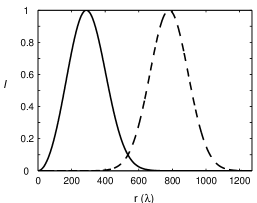
Figure 1: Dependence of normalized transverse intensity on the radial coordinate at the focal plane, where $kw_{0}=1000$ and $r$ is in units of wavelength $\lambda$. Solid: $\beta=0.002k$; dashed: $\beta=0.005k$.

To the best of our know, this is the first time to observe theoretically the above-mentioned 2 kinds of vector beam. Since the modified-Bessel-Gaussian scalar beams show an elongated diffraction-free region Ruschin in comparison with the fundamental Gaussian beam, the propagation properties of the modified-Bessel-Gaussian vector beams deserve investigation in detail. This is beyond the scope of this paper and will be presented elsewhere.

3 Bessel-Gaussian vector beams With a modification factor containing the modified Bessel function of the first kind of order one,

$$A_{m}=\exp\left(-\frac{w^{2}_{0}}{2}\beta^{2}\right)I_{1}(\beta w^{2}_{0}k_{\rho}),$$

we find

$$E_{T}(r,x)=\frac{A_{0}}{w^{2}}J_{1}(\frac{w^{2}_{0}}{w^{2}}\beta r)\exp\left[-\frac{1}{2w^{2}}(r^{2}+i\beta^{2}w^{2}_{0}\frac{x}{k})\right].$$

If $\tilde{l}=\left(\begin{array}[]{c}1\\ 0\end{array}\right)$, we arrive at the azimuthally polarized $J_{1}$ Bessel-Gaussian vector beam, the same as was obtained by solving the paraxial wave equation Jordan .

4 Laguerre-Gaussian vector beams Furthermore, with a modification factor containing the associated Laguerre polynomial,

$$A_{m}=\frac{k_{\rho}}{k}L^{1}_{n}(-\frac{\alpha^{2}}{2}k^{2}_{\rho}),$$

where $\alpha$ is a constant, we have

$$E_{T}(r,x) = \frac{A_{0}}{kw^{4}}\left(1+\frac{\alpha^{2}}{w^{2}}\right)^{n}r\times$$

$$\exp\left(-\frac{r^{2}}{2w^{2}}\right)L^{1}_{n}\left(-\frac{\alpha^{2}}{w^{2}+\alpha^{2}}\frac{r^{2}}{2w^{2}}\right).$$

This kind of vector beam includes the axisymmetric Laguerre-Gaussian vector beam discussed in Ref. Tovar .

When the amplitude two-form $\tilde{A}$ depends on the azimuthal variable $\varphi$ in the wavevector space, the vector beam produced by Eq. (3) will in general be no longer axisymmetric. Suitable choices will lead to cylindrical vector beams of topological charges Stalder ; Hall ; Tovar .

This work was supported in part by the National Natural Science Foundation of China (Grant 60377025), Science and Technology Commission of Shanghai Municipal (Grant 04JC14036), and the Shanghai Leading Academic Discipline Program (T0104).

References

- (1) P. L. Greene and D. G. Hall, J. Opt. Soc. Am. A 15, 3020 (1998).
- (2) K. Youngworth and T. Brown, Opt. Express 7, 77 (2000).
- (3) R. Dorn, S. Quabis, and G. Leuchs, Phys. Rev. Lett. 91, 233901 (2003).
- (4) H. Guo, J. Chen, and S. Zhuang, Opt. Express 14, 2095 (2006).
- (5) A. Ashkin, IEEE J. Sel. Top. Quantum Electron. 6, 841 (2000).
- (6) Q. Zhan and J. R. Leger, Appl. Opt. 41, 4630 (2002).
- (7) D. P. Biss, K. S. Youngworth, and T. G. Brown, Appl. Opt. 45, 470 (2006).
- (8) L. W. Davis and G. Patsakos, Opt. Lett. 6, 22 (1981).
- (9) R. H. Jordan and D. G. Hall, Opt. Lett. 19, 427 (1994).
- (10) D. G. Hall, Opt. Lett. 21, 9 (1996).
- (11) A. A. Tovar and G. H. Clark, J. Opt. Soc. Am. A 14, 3333 (1997).
- (12) A. A. Tovar, J. Opt. Soc. Am. A 15, 2705 (1998).
- (13) M. A. Bandres and J. C. Gutiérrez-Vega, Opt. Lett. 30, 2155 (2005).
- (14) C.-F. Li, Phys. Rev. A 76, 013811 (2007).
- (15) R. Martínez-Herrero, P. M. Mejías, S. Bosch, and A. Carnicer, J. Opt. Soc. Am. A 18, 1678 (2001).
- (16) M. Lax, W. H. Louisell, and W. B. McKnight, Phys. Rev. A 11, 1365 (1975).
- (17) J. Enderlein and F. Pampaloni, J. Opt. Soc. Am. A 21, 1553 (2004).
- (18) G. E. Andrews, Richard Askey, and R. Roy, Special Functions (Cambridge University Press, 2000), p. 216
- (19) S. Ruschin, J. Opt. Soc. Am. A 11, 3224 (1994).
- (20) M. Stalder and M. Schadt, Opt. Lett. 21, 1948 (1996).