Single-Particle Dynamics in the Vicinity of the Mott-Hubbard Metal-to-Insulator Transition

Abstract

The single-particle dynamics close to a metal-to-insulator transition induced by strong repulsive interaction between the electrons is investigated. The system is described by a half-filled Hubbard model which is treated by dynamic mean-field theory evaluated by high-resolution dynamic density-matrix renormalization. We provide theoretical spectra with momentum resolution which facilitate the comparison to photoelectron spectroscopy.

I Introduction

Strongly correlated systems are notoriously difficult to understand. In particular, this is true when parameter regions are considered where the system changes its behavior qualitatively, for instance where new excitations emerge. This is precisely the situation around the metal-to-insulator transition of electrons which repel each other strongly on a tight-binding lattice due to the Coulomb interaction.

We consider a half-filled lattice with one electron per site on average. For strong on-site repulsion, it is energetically forbidden that two electrons occupy the same site. Because there is one electron per site on average this implies that there is precisely one electron per site. No electron can move so that the system is insulating. The remaining degree of freedom is the orientation of the electron spins. This freedom gives rise to collective magnetic excitations, for instance spin waves.

For weak interaction, on the other hand, the system is a metal in the sense of a Fermi liquid. This is true if we neglect ordering phenomena, i.e., we focus on the paramagnetic phase. Hence this system is dominated by the quasiparticle excitations. No collective modes play a major role.

In the vicinity of the metal-to-insulator transition the Fermi liquid must change such that precursors of the collective magnetic excitations of the insulator emerge. Vice versa, the collective excitations in the insulator must acquire finite life times so that they broaden considerably in the corresponding spectra if we pass in the insulating regime towards the metallic one. Such behavior can be measured by inelastic neutron scattering for example.

Hence it is of particular interest to understand the dynamics of the important excitations in the vicinity of an interaction induced metal-to-insulator transition. In the present work, we focus on the single-particle excitations, that means we investigate the single particle propagation. The investigation is done in the framework of the dynamic mean-field theory (DMFT) which maps the lattice model to an effective single site problem with a self-consistency condition.Metzner and Vollhardt (1989); Müller-Hartmann (1989); Georges and Kotliar (1992a); Jarrell (1992) The single site is coupled to a bath of non-interacting fermions which can be represented as a semi-infinite chain.

The semi-infinite chain and its head where the interaction takes place can be tackled numerically by algorithms for one-dimensional systems. We will use density-matrix renormalization for this purpose. White (1992, 1993) Since the dynamic properties have to be determined we use the dynamic density-matrix renormalization with correction vector. Ramasesha et al. (1997); Kühner and White (1999) Thereby, we dispose of a numerical means which can resolve spectral properties not only at low energies but also at high energies.Raas et al. (2004) This makes it possible to determine sharp spectral features away from the Fermi energy also quantitatively.Karski et al. (2005)

The main aim of the present article is to provide comprehensive spectral data in the above mentioned theoretical framework. In particular, we present momentum-resolved single-particle spectral densities in the insulating and in the metallic regime.

In the following Sec. I.1, we will present the model under investigation, i. e. the half-filled one-band Hubbard model with semi-elliptic density of states (Bethe lattice) at zero temperature. Next, in Sec. II, we will discuss the method. We use the dynamic mean-field theory (DMFT, Sec. II.1) which maps the problem to an effective single-impurity Anderson model (SIAM, Sec. II.2) with a self-consistency condition. The SIAM is treated numerically by a dynamic density-matrix renormalization (D-DMRG) impurity solver (Sec. II.3). The results of this approach are presented in Sec. III, with the spectral properties in the paramagnetic insulating phase (Sec. III.1) and the paramagnetic metallic phase (Sec. III.2). The results reveal insights in the nature of the Mott-Hubbard metal-to-insulator transition and provide a numerical proof for previous investigations which were based on the hypothesis of the separation of energy scales. Finally, a summary will be given in Sec. IV.

I.1 Model

We use the generic model for strongly correlated systems in solids, namely the Hubbard model.Kanamori (1959); Hubbard (1963); Gutzwiller (1963) It is given by the Hamiltonian

$$\mathcal{H}=U\sum_{i}\left(n_{i,\uparrow}-\nicefrac{{1}}{{2}}\right)\left(n_{i,\downarrow}-\nicefrac{{1}}{{2}}\right)-t\sum_{\langle i,j\rangle,\sigma}c^{\dagger}_{i,\sigma}c^{\phantom{\dagger}}_{j,\sigma}$$ (1)

where $i$, $j$ denote sites on a lattice with $\langle i,j\rangle$ being nearest neighbors, $\sigma\in\{\uparrow,\downarrow\}$ the spin and $c^{(\dagger)}_{i;\sigma}$ the electron annihilation (creation) operator and $n_{i;\sigma}$ their occupation operator. This model contains the basic ingredients of the problem, i.e., a local repulsive interaction and a kinetic energy consisting of hopping from site to site. The interaction is diagonal in real space and hence tends to make the eigenstates local in real space. The kinetic energy is diagonal in momentum space and hence tends to make the eigenstates local in momentum space implying extended states in real space. So the interaction favors an insulating phase whereas the kinetic energy favors a conducting, metallic phase. They are the antagonists and depending on their relative strength the system is metallic or insulating.

The transition between these two phases has been a long-standing issue. By now, evidence emerges that the transition is continuous at zero temperature Kotliar (1999); Karski (2004); Karski et al. (2005) whereas it is of first order at any finite temperature.Potthoff (2003) The continuous transition at zero temperature is peculiar. It cannot be seen as an ordinary second-order transition. It should rather be seen as a marginal first-order transition with zero hysteresis. At zero temperature, the free energy is continuously differentiable at the transition because the ground-state energy is continuously differentiable. The residual entropy jumps even at zero temperature because the ground-state of the metal is the non-degenerate Fermi sea. The insulator, however, is governed by the spin degrees of freedom. Since we do not consider any long-range order they remain free down to zero energy. The freedom to choose the spin locally $\uparrow$ or $\downarrow$ in the paramagnetic insulating phase implies a finite residual entropy of $\ln 2$ per site. But at zero temperature, the discontinuous entropy does not imply jumps in the other thermodynamic quantities.

II Method

In this section we present the details of the methods that we used to tackle the model and to compute the desired single-particle dynamics. The key points are the dynamic mean-field theory, the single-impurity Anderson model and the dynamic density-matrix renormalization.

II.1 Dynamic mean-field theory

The basic idea of the dynamic mean-field theory is to consider the lattice problem under study in the limit of infinite coordination number $z\to\infty$. This means that the lattice is generalized in a way that $z$ is a tunable parameter. Very often, this is realized by considering related lattices in $d$-dimensional space. Then $z\propto d$ and the desired limit is the limit of infinite dimensions.

The limit $z\to\infty$ is well-defined only for a particular scaling of the matrix elements in the Hamiltonian (1) which link different sites. In particular, the hopping to the nearest-neighbors must be scaled like $1/\sqrt{z}$.Metzner and Vollhardt (1989); Müller-Hartmann (1989) Then the single-particle propagator $G_{ij}$ between site $j$ and site $i$ scales like

$$G_{ij}\propto z^{||i-j||/2}$$ (2)

where we use $||i-j||$ for the taxi cab metric. This metric counts how many hopping processes are at least necessary to go from $j$ to $i$.

Considering the standard diagrammatic expansion in powers of the interaction one realizes that the scaling (2) implies that many diagrams vanish for $z\to\infty$. Only those which are either completely local or which are sufficiently numerous lead to non-vanishing contributions. Closer inspection shows that only those dressed skeleton diagrams lead to non-vanishing contributions which are completely local.Metzner and Vollhardt (1989); Müller-Hartmann (1989) This is called the collapse of the diagrams because only a single site occurs. For the proper self-energy $\Sigma$ this implies that it is local; only $\Sigma_{ii}$ needs to be considered.

In spite of the very substantial reduction of the number of relevant diagrams their summation is not directly possible. Hence the dynamic mean-field theory requires an additional element. This is the observation that the same local dressed skeleton diagrams occur in the treatment of a single-impurity Anderson model (SIAM) where the interaction takes place at the impurity which is coupled to a fermionic bath.Georges and Kotliar (1992a); Jarrell (1992); Uhrig (1996) Hence, the same self-energy is obtained if the local dressed propagators are the same. Let us use capital letters for the local dressed propagator $G:=G_{ii}$ and for the local self-energy $\Sigma:=\Sigma_{ii}$ in the lattice model in DMFT. We use small letters for the local dressed propagator $g$ and the self-energy $\sigma$ at the impurity of the effective single-site problem. Then the above statement reads

$$\Sigma(\omega)=\sigma(\omega)$$ (3a)

if

$$G(\omega)=g(\omega)$$ (3b)

holds. Note that this does not imply that $G^{0}=g^{0}$ where we use the superscript ⁰ for the bare, undressed propagators.

For completeness, we mention that the self-consistency equations (3), which we derived from the expansion in dressed skeleton diagrams, can also be obtained from the action by the so-called cavity argument.Georges et al. (1996) A derivation in the strong coupling limit is given in the review Georges et al., 1996. An elegant derivation of the DMFT including the possibility to generalize from single site to cluster systems has been found by Potthoff Potthoff (2003) in the framework of variational self-energy functionals.

Eqs. (3) face us with the problem that we do not know the bare propagator of the SIAM. This amounts up to a generic self-consistency problem where we first have to guess a $g^{0}$ and then we can verify whether the conditions (3) are fulfilled.

Following this roadmap, two more fundamental relations are needed, namely the Dyson equations of the lattice problem and of the SIAM. The local self-energy $\Sigma_{ii}$ acts on every site equally since we consider the uniform, paramagnetic phase. For this reason we could omit the subscript and pass on to $\Sigma$. This spatially constant energy acts like a global energy shift so that it can be accounted for by

$$G(\omega)=G^{0}(\omega-\Sigma(\omega)),$$ (4)

which is the Dyson equation for the lattice problem.

In the single-site problem, the self-energy $\sigma(\omega)$ acts only on the impurity site. The bare propagator from the impurity site to the impurity site is $g^{0}(\omega)$ so that the Dyson equation is given by the geometric series

$$g(\omega) = g^{0}+g^{0}\sigma g^{0}+g^{0}\sigma g^{0}\sigma g^{0}+\ldots+g^{0}(\sigma g^{0})^{n}+\ldots$$ (5)

$$= \frac{g^{0}(\omega)}{1-g^{0}(\omega)\sigma(\omega)}.$$

This relation can also be written as

$$\nicefrac{{1}}{{g}}=\nicefrac{{1}}{{g^{0}}}-\sigma.$$ (6)

The above equations are used to set up an iteration cycle to find a self-consistent solution. It is illustrated in Fig. 1.

Figure 1: Schematic representation of the iterative self-consistency cycle for an arbitrary lattice. In the step marked with ★ the dynamics of an effective single-impurity Anderson model is calculated by a D-DMRG impurity solver.

Starting in the upper left corner, an initial guess is used to define the SIAM which is then solved by an impurity solver providing $\sigma$. Then $\sigma$ is used as lattice self-energy $\Sigma$ providing via the lattice Dyson equation (4) the dressed propagator for the lattice. By the condition (3b) the dressed propagator of the SIAM is known which in turn yields via (6) its bare counterpart so that we are at the beginning of the cycle again. If the bare propagator is close enough to the previous assumption the iterations are stopped. Details of the precise meaning of how close is close enough are given in Sec. II.3.4.

The above sketched cycle can be used for any lattice, i.e., for any $G^{0}$. For a particular $G^{0}$ with semi-elliptic spectral density (DOS) $\rho^{0}(\omega):=\nicefrac{{-1}}{{\pi}}\mathfrak{Im}G^{0}(\omega)$

$$\rho^{0}(\omega)=\frac{2}{\pi D^{2}}\sqrt{D^{2}-\omega^{2}},$$ (7)

the cycle can be simplified considerably. A semi-elliptic spectral density $\rho^{0}(\omega)$ corresponds to the so-called Bethe lattice with infinite branching ratio.Economou (1979) Note that we do not use any other feature from the Bethe lattice other than (7). Hence our calculation can be viewed as treating a translationally invariant lattice with a semi-elliptic DOS. This is a good starting point for generic spectral densities since it is bounded and it possesses square-root singularities at the band edges like three-dimensional densities-of-states have. Otherwise it is featureless.

The key feature of $G^{0}$ with semi-elliptic $\rho^{0}(\omega)$ is its particularly simple continued fraction representation with constant coefficients

$$G^{0}(\omega)=\frac{1}{\omega-{\displaystyle\frac{\nicefrac{{D^{2}}}{{4}}}{\omega-{\displaystyle\frac{\nicefrac{{D^{2}}}{{4}}}{\omega-\cdots}}}}}.$$ (8)

In order to use this fact for simplification we write the bare propagator of the SIAM with the help of the so-called hybridization function $\Gamma(\omega)$ as

$$g^{0}(\omega)=\frac{1}{\omega-\Gamma(\omega)}$$ (9)

where the continued fraction of $\Gamma(\omega)$ shall be parametrized like

$$\Gamma(\omega)=\frac{V^{2}}{\omega-{\displaystyle\frac{\gamma_{0}^{2}}{\omega-{\displaystyle\frac{\gamma_{1}^{2}}{\omega-\cdots}}}}}.$$ (10)

Then, based on Eqs. (6,3a) the dressed propagator of the SIAM reads

$$\frac{1}{g(\omega)}=\omega-\Gamma(\omega)-\Sigma(\omega).$$ (11)

By Eqs. (4,8) the dressed propagator of the lattice can be expressed to be

$$\frac{1}{G(\omega)} = \omega-\Sigma(\omega)-\frac{\nicefrac{{D^{2}}}{{4}}}{\omega-\Sigma-{\displaystyle\frac{\nicefrac{{D^{2}}}{{4}}}{\omega-\Sigma-{\displaystyle\frac{\nicefrac{{D^{2}}}{{4}}}{\omega-\Sigma\cdots}}}}}$$ (12)

$$= \omega-\Sigma(\omega)-\left(\nicefrac{{D^{2}}}{{4}}\right)G(\omega),$$

where we exploited that the continued fraction does not change when it is evaluated at a deeper level because its coefficients are constant.

Based on the self-consistency condition (3b) we set Eqs. (11,12) equal and obtain the simpler self-consistency condition

$$\Gamma(\omega)=\frac{D^{2}}{4}G(\omega).$$ (13)

This equation is more easily used because it provides a direct way to compute the hybridization function $\Gamma(\omega)$ of the next iteration of the SIAM from the dressed lattice propagator $G$. No explicit computation of intermediate self-energies is needed which can be severely hampered by numerical errors, see below. A first conclusion which can be drawn from (13) is that $V=D/2$.

The resulting cycle is given graphically in Fig. 2. This form of the iteration cycle is used in the present work.

Figure 2: Schematic representation of the iterative self-consistency cycle for semi-elliptic density of states (DOS) with nearest-neighbor hopping. The step ★ stands for the D-DMRG impurity solver.

II.2 Single-Impurity Anderson Model

There are various ways to set up the effective single-impurity problem because the precise topology of the fermionic bath, to which the impurity couples, does not matter. As we have seen in the equations above we are only concerned with the local quantities on the impurity. Hence the only relevant property of the fermionic bath is the bare propagator $g^{0}$ or the hybridization function $\Gamma$, respectively.

Because we aim at the application of density-matrix renormalization, which has been developed for one-dimensional systems in particular, we favor the representation of the bath as semi-infinite chain, see Fig. 3.

Figure 3: (Color online) Sketch of the semi-infinite chain which is used as topology for the single-impurity Anderson model.

This is no restriction since mathematically any hybridization function which has a non-negative spectral density can be represented as continued fraction Pettifor and Weaire (1985) as given in Eq. (10). By complete induction it is straightforward to see that the choice of the hopping elements shown in Fig. 3 implies Eq. (10).

The Hamiltonian of the SIAM represented as linear chain readsHewson (1993)

$$\mathcal{H}=U\left(n_{d,\downarrow}-\nicefrac{{1}}{{2}}\right)\left(n_{d,\uparrow}-\nicefrac{{1}}{{2}}\right)+V\sum_{\sigma}\left(d_{\sigma}^{\dagger}c_{0,\sigma}^{\phantom{\dagger}}+\text{h.c.}\right)$$

$$+\sum_{n=0,\,\sigma}^{\infty}\gamma_{n}\left(c_{n,\sigma}^{\dagger}c_{n+1,\sigma}^{\phantom{\dagger}}+\text{h.c.}\right).$$ (14)

The correlations stem from the density-density coupling on the impurity site ($d^{(\dagger)}$ operators) at the head of a semi-infinite chain of free fermions ($c^{(\dagger)}$ operators). For comprehensive information on the physics of single-impurity Anderson models the reader is referred to Ref. Hewson, 1993.

The determination of the local propagator $g(\omega)$ in the effective SIAM (14) for a given hybridization function $\Gamma(\omega)$ is the most difficult part in the self-consistency cycles (cf. Figs. 1 and 2). The necessary tool is called the impurity solver.

The dynamics one has to compute is the dynamics of the fermionic single-particle propagator of the impurity electron. Aiming at the properties at $T=0$ it reads

$$\begin{split}g(\omega+\mathrm{i}\eta)=&\left\langle 0\left|d_{\sigma}\frac{1}{\omega+\mathrm{i}\eta-(\mathcal{H}-E_{0})}d^{\dagger}_{\sigma}\right|0\right\rangle\\ +&\left\langle 0\left|d^{\dagger}_{\sigma}\frac{1}{\omega+\mathrm{i}\eta+(\mathcal{H}-E_{0})}d_{\sigma}\right|0\right\rangle\ .\end{split}$$ (15)

Here the ground-state is denoted by $|0\rangle$ and its energy by $E_{0}$. Since we aim at the paramagnetic phase the propagator has no dependence on the spin index $\sigma$ and we do not denote it. The frequencies $\omega$ and $\eta$ are real. The standard retarded propagator is retrieved for $\eta\to 0+$

$$g_{\text{R}}(\omega)=\lim_{\eta\to 0+}g(\omega+\mathrm{i}\eta).$$ (16)

The wanted quantity is the spectral density $\rho(\omega):=-\pi^{-1}\mathfrak{Im}\,g_{\text{R}}(\omega)$. If necessary the real part of $g_{\text{R}}(\omega)$ can be obtained from $\rho(\omega)$ by the Kramers-Kronig relation

$$\mathfrak{Re}\,g_{\text{R}}(\omega)=\mathcal{P}\int\limits_{-\infty}^{\infty}\frac{\rho(\omega^{\prime})}{\omega-\omega^{\prime}}\,\mathrm{d}\omega^{\prime},$$ (17)

where $\mathcal{P}$ denotes the principal value.

II.3 Dynamic Density-Matrix Renormalization

II.3.1 Algorithm

Because there are essentially no analytic approaches available which solve the general SIAM, reliable numerical approaches for dynamic correlations are very important. Our choice is the dynamic density-matrix renormalization which is an excellent tool for calculations for open one-dimensional systems at zero temperature.

To obtain $g(\omega)$ for a given $\Gamma(\omega)$ we use a combination of the dynamic density-matrix renormalizationHallberg (1995); Ramasesha et al. (1997); Kühner and White (1999) (D-DMRG) and the least-bias deconvolution algorithm.Raas and Uhrig (2005) The D-DMRG is the generalization of the standard density-matrix renormalization groupWhite (1992, 1993) (DMRG) for the calculation of dynamic quantities. A key advantage over other $T=0$ approaches like the numerical renormalization group is that the resolution can be high not only at low energies but also at high energies.Raas et al. (2004) We implemented the D-DMRG in a correction vector (CV) schemeRamasesha et al. (1997); Kühner and White (1999); Hövelborn (2000) with optimized direct matrix inversion, for details see Refs. Raas et al., 2004 and Raas, 2005.

The actual calculations are not performed for the fermionic representation (14) but for a spin representation involving two semi-infinite spin chains which are coupled at their heads. This spin representation replaces each fermionic level with states empty and occupied by the two spin states $\uparrow$ and $\downarrow$. The change of basis between both representations is accomplished by two Jordan-Wigner transformations, one for the $\uparrow$ electrons and one for the $\downarrow$ electrons, see Ref. Raas et al., 2004. The resolvents appearing in Eq. (15) are expressed as resolvents of the equivalent spin system involving spin flips at the head of the chains. The advantage for the DMRG approach is that in the spin chain description each site carries only a two dimensional Hilbert space instead of a four dimensional one.

The correction vector D-DMRG provides data points at given frequencies $\omega=\omega_{i}$ for finite values of $\eta=\eta_{i}$

$$g_{i} := -\frac{1}{\pi}\mathfrak{Im}\,g(\omega_{i}+\mathrm{i}\eta_{i})$$ (18a)

$$= \rho(\omega)\otimes L_{\eta_{i}}(\omega)\Big{|}_{\omega=\omega_{i}}$$ (18b)

$$= \frac{1}{\pi}\int\limits_{-\infty}^{\infty}\frac{\eta_{i}\rho(\omega)\mathrm{d}\omega}{(\omega-\omega_{i})^{2}+\eta_{i}^{2}},$$ (18c)

where $\otimes L_{\eta_{i}}(\omega)$ stands for the convolution with a Lorentzian of width $\eta_{i}$. No data can be obtained directly at $\eta=0$ since the inversion of the Hamiltonian is singular and cannot be achieved numerically in a stable way. Furthermore, we cannot numerically treat an infinite chain but only a finite one.

Henceforth, we will call data $\{g_{i}\}$ raw data because it is obtained at finite values of $\eta_{i}$. Apart from the constraint from matrix inversion, a sufficiently large broadening $\eta_{i}$ is used in order to calculate continuous spectral densities resembling the spectral densities in the thermodynamic limit. The finite-size effects are washed out. In a second step, we aim at retrieving the unbroadened spectral density $\rho(\omega)$ as well as possible.

We use the D-DMRG raw data calculated for a finite set of frequencies $\omega_{i}$ with non-zero broadenings $\eta_{i}$ as input of a deconvolution scheme to extract the information on the spectral density $\rho(\omega)$, i. e. the relevant dynamic properties of the infinite system. The deconvolution scheme of our choice is the least-bias (LB) approach Raas and Uhrig (2005) which belongs to the class of maximum entropy methods.Press et al. (1992) The combination of D-DMRG and LB deconvolution has already proven itself in the investigation of the high-energy dynamics of the SIAM by providing a well-controlled resolution for all energies.Raas and Uhrig (2005); Raas (2005) By construction, the LB ansatz yields a positive and continuous result for the density of states $\rho(\omega)$ (DOS). The positiveness assures the causality of the solution, which is necessary for calculating the continued fraction, see App. A, whereby the DMFT self-consistency cycle is closed. By using the LB deconvolution we avoid any kind of arbitrariness introduced by the choice of a discretization mesh.

Of course, the direct computation of a continuous density from data obtained for a finite system involves an approximation. In practice, one must pay attention whether the system size and the broadening considered make it possible to deduce continuous densities, see also below.

Nishimoto and co-workers Nishimoto et al. (2004, 2006) advocate a different approach which has been baptized “Fixed-Energy” DMFT where the problem of deducing densities is circumvented by discretizing the continuous frequency in a number of bins. For these bins the spectral weights are computed. On the one hand, spectral weights are better behaved for finite system sizes. But on the other hand, the DMFT self-consistency holds only for the continuous quantities in Eq. (3). So any extension to discrete quantities introduces some ambiguity.Eastwood et al. (2003) Balancing these two contrary aspects we have chosen to work with the continuous spectral densities as obtained from the LB ansatz.

In the framework of the D-DMRG Jeckelmann has formulated a variational principle for the wanted dynamic correlation.Jeckelmann (2002) A certain functional is minimum for the correct dynamic correlation. Its value yields the $g_{i}$ as defined in (18a). Due to the minimum principle this approach is rather robust. Its main advantage is that even if the numerical dynamic correlation possesses an error $\delta$ the values $g_{i}$ will be exact up to quadratic order $\delta^{2}$. From the algorithmic view point the minimization required for Jeckelmann’s approach is more demanding than the matrix inversion in the D-DMRG with correction vector. Hence we stick to an optimized matrix inversion. Raas et al. (2004); Raas (2005) In our opinion, the optimum strategy is to search for the best correction vector by optimized matrix inversion and then to use the variational functional for the evaluation of the $g_{i}$.

II.3.2 Deconvolution and Finite-Size Effects

The choice of the $\eta_{i}$ for a given set of $\omega_{i}$ is restricted by the considered chain length $L$. If the $\eta_{i}$ are chosen too small, the extracted spectral properties reveal too strong finite-size effects. If the $\eta_{i}$ are chosen too large, essential features in the spectral properties cannot be resolved properly and therefore remain smeared out, even after the deconvolution. Thus, the optimum value of each $\eta_{i}$ has to been chosen with care depending on the width of the features which have to be resolved. In our approach the optimum choice is characterized by

$$\eta_{i}\approx\Delta\omega_{i}\gg W^{*}/L$$ (19)

where $\Delta\omega_{i}$ denotes the distance between two neighboring frequencies and $W^{*}$ is the bandwidth. The approximate equality between $\eta_{i}$ and $\Delta\omega_{i}$ reflects the fact that it is not reasonable to numerically measure the spectral density which is broadened by $\eta_{i}$ at frequencies much closer than $\eta_{i}$. This does not lead to an increase of relevant information about the underlying unbroadened spectral density. In contrast, it might happen that small errors lead to inconsistencies of the too closely positioned data points so that the subsequent deconvolution leads to strongly oscillatory results.Raas and Uhrig (2005)

The inequality $\Delta\omega_{i}\gg W^{*}/L$ in (19) results from the approximation of the infinite system under study by a finite system. If the points $\omega_{i}$, at which the broadened spectral density is measured numerically, were too closely spaced the finite-size effects would be discernible. Hence the raw data $\{g_{i}\}$ could not be processed as if it resulted from a continuous spectral density.

Finally, we point out, that apart from the resolution aspect, the choice of $\eta_{i}$ influences the stability and the performance of the correction vector D-DMRG. For very small values of $\eta_{i}$ the matrix inversions are numerically very demanding and time-consuming.

II.3.3 Continuous Fraction

The LB algorithm and the Kramers-Kronig transformation allow us to extract the full unbroadened Green function $g(\omega)$ to good accuracy from the raw D-DMRG data for an arbitrary $\omega$. Thus we can have an arbitrary number of supporting points for further numerical calculations. The hopping elements $\gamma_{n}$ of the effective SIAM (14) for the next iteration in the self-consistency cycle are calculated recursively by a continued fraction expansion.Pettifor and Weaire (1985); Viswanath and Müller (1994) Note, that even tiny regions of small negative spectral density spoil the continued fraction expansion completely. The details of the calculation of the continued fraction are given in App. A.

II.3.4 Numerical Criteria for Self-Consistency

We have realized the iterative cycle shown in Fig. 2. Since we perform the calculation of the spectral densities numerically, including an advanced deconvolution scheme, the calculation of two identical spectral densities within the iterative self-consistency cycle is not possible by principle. Consequently, a certain error tolerance has to be included to the termination conditions.

A solution within our DMFT self-consistency cycle is understood as self-consistent, if at least the following conditions are fulfilled:

1. Two deconvolved spectral densities calculated consecutively within the self-consistency cycle obey for all $\omega$,

   $$|\rho^{(i)}(\omega)-\rho^{(i+1)}(\omega)|<\varepsilon\ ,$$ (20)

   where $\varepsilon=4\times 10^{-3}/D$ for the metallic and $\varepsilon=10^{-3}/D$ for the insulating solutions.

2. The average double occupancy and the ground-state energy per lattice site calculated in succession within the self-consistency cycle are stable. That means that they differ by less than $10^{-2}\%$.

For the insulating solutions, we additionally require that the static single-particle gaps calculated consecutively by means of the standard DMRG algorithm differ by less then $1\%$. The higher value of $\varepsilon$ for the metallic solutions has to be chosen because the metallic spectral densities display a high complexity including many sharp features. In contrast, the spectral densities of the insulating solutions are rather featureless and thus converge more easily.

We stress that the upper conditions are the minimum requirement and that most of our solutions surpass them considerably. But we observed that it is sufficient to terminate the self-consistency cycle once the upper conditions are fulfilled. The physical quantities obtained from the continued fractions computed in two consecutive iterations are almost identical. Further iterations yield no further improvement. Moreover, we have confirmed that our final continued fraction coefficients do not display persistent trends of change if iterated further. They rather display very small oscillations around the results which we consider to be converged.

II.3.5 Numerical Stability of the Metallic and the Insulating Solution

There is a parameter region in the Hubbard model in infinite dimensions with an interaction $U$ between $U_{\text{c1}}$ and $U_{\text{c2}}$ where both solutions are locally stable. In a numerical treatment of this situation one has to introduce a bias, preferably minute, which selects the solution we want to find.

This can be done elegantly by exploiting an even-odd effect. If we consider only the impurity site, the bare DOS $\rho^{0}(\omega)$ consists of a single $\delta$-peak at $\omega=0$. Any arbitrary finite repulsion $U>0$ splits this peak into two so that a gap $\Delta=U/2$ occurs. The corresponding self-energy has a pole at $\omega=0$ which is necessary to induce the splitting of the central peak. Hence this self-energy is the self-energy of an insulator.

Any SIAM with an odd number of fermionic sites (one impurity site and an even number of bath sites) has a bare DOS $\rho^{0}(\omega)$ with a $\delta$-peak at $\omega=0$. This lowest energy level can be occupied or unoccupied without changing the ground-state energy. A finite repulsive interaction will lift this degeneracy partly and split the central $\delta$-peak in two and a gap occurs. Of course, if the levels in the bare system lie very close to each other the occurring gap can be very small. But in any case, the solution resembles an insulating one. We conclude that the use of a SIAM with an odd number of sites implies a small bias towards an insulating solution. Obviously, the relative bias is of the order of the inverse system size $1/L$.

Conversely, considering a SIAM with an even number of sites amounts up to a small bias towards a self-energy belonging to a metallic phase. The imaginary part of $\Sigma$ at $\omega=0$ is zero.

While the metallic solutions correspond to the Fermi sea as unique ground-state the paramagnetic insulating solution implies a macroscopically large degeneracy in the lattice problem. In the SIAM, the degeneracy is only two. It stems from the fact that the spin of the impurity is not completely screened by the coupling to the bath because the bath is gapped by $\Delta$. So there is no DOS at low energies and the renormalization of the unscreened moment stops at the lower cut-off $\Delta$. Indeed, we found that the insulating baths show a two-fold degenerate ground-state or two almost degenerate low-lying states.

The spin degeneracy in the insulator poses a problem to the numerical treatment. It happens easily that the DMRG algorithm looking for the ground-state provides a state with a certain finite magnetization in $z$-direction. If such a solution is used further in the iteration cycle results are produced which do not describe the paramagnetic insulating phase. In order to avoid this problem, we first search for the ground-state $|1\rangle$ with energy $E_{1}$ using a standard Lanczos or Davidson algorithm starting from an initial guess $|I_{1}\rangle$. The degenerate or almost degenerate second state $|2\rangle$ is found from a second run starting from the orthogonal initial guess $|I_{2}\rangle=|I_{1}\rangle-\langle 1|I_{1}\rangle|1\rangle$. With both states we can construct a ground-state without magnetization. We use the normalized superposition $|0\rangle=\alpha_{1}|1\rangle+\alpha_{2}|2\rangle$ with $1=|\alpha_{1}|^{2}+|\alpha_{2}|^{2}$ where the coefficients are chosen such that

$$\left\langle 0\left|d_{\sigma}^{\phantom{\dagger}}d_{\sigma}^{\dagger}\right|0\right\rangle=\nicefrac{{1}}{{2}}.$$ (21)

for $\sigma=\{\uparrow,\downarrow\}$ which ensures the absence of a magnetization in $z$-direction.

Finally, we note that the treatment of the spectral density in the region of the single-particle gap $\Delta$ in the insulating phase requires care. The LB deconvolution scheme does not allow for zero spectral density so that some artifacts need to be removed before the continued fraction expansion can be calculated as explained in Appendix A. The details of the removal of deconvolution artifacts are given in App. B.

III Results

Here we present the results for various spectral densities which we have obtained by the approach described so far. First we focus on the insulating solutions; then we pass on to the metallic solutions. The results are interpreted as well as compared to previous results.

III.1 Insulator

III.1.1 Local Spectral Densities

The computation of the insulating spectral densities is performed for $121$ fermionic sites, including the impurity. Larger system sizes provide identical solutions (not shown). This is related to the relatively low complexity of the insulating solutions which do not display particular features besides the insulating gap.

We calculate the raw D-DMRG data on a grid using mostly $\Delta\omega_{i}=\eta_{i}=0.1D$. Close to the edges of the Hubbard bands we increase the resolution by choosing $\Delta\omega_{i}=\eta_{i}=0.05D$ and partially $0.025D$ or even $\Delta\omega_{i}=\eta_{i}=0.01D$ for $U=2.4D$. This is done to resolve the gap and the band edges properly. Note, that such a small broadening is useful here, although $\eta_{i}=0.01D$ does not obey the inequality (19), because it helps to decide where the spectral density is finite or zero.

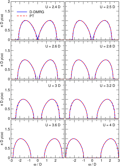
Figure 4: (Color online) Spectral densities $\rho(\omega)$ in the insulating regime (solid line) calculated with a chain of $121$ fermions. The dashed lines (almost coinciding) show the results from strong coupling perturbation theory.Gebhard et al. (2003)

The insulating solutions in Fig. 4 clearly show the lower and the upper Hubbard band each with a band width of nearly $2D$. The bands are separated by a well pronounced gap of $2\Delta$. The center of each Hubbard band is located at roughly $\omega=\pm\nicefrac{{U}}{{2}}$. The shape of the density in the Hubbard bands in our insulating solutions is essentially smooth and reveals no significant features. They agree very well with the perturbative results by Gebhard et al.  Gebhard et al. (2003) which are based on a strong coupling expansion in $\nicefrac{{1}}{{U}}$. Only for very small gaps $\Delta\approx 0.2D$ a noticeable deviation is discernible, see Fig. 5. Clearly, these deviations result from the limited number of terms which are available in the perturbation series.

Figure 5: (Color online) Data from Fig. 4 on a zoomed scale close to the inner band edges.

In Ref. García et al., 2004 a DMFT calculation based on another DMRG impurity solver, the Lanczos method, showed many substructures in the Hubbard bands. The comparison to our featureless bands leads us to the conclusion that the peaky substructures in Ref. García et al., 2004 stem from finite-size effects. First, such effects enter because only 45 fermionic sites were considered. Second, the reliable application of the Lanczos impurity solver would require a large number ($\approx 100$) of target states which cannot be handled by the DMRG.

The results in Ref. Nishimoto and Jeckelmann, 2004 differ from ours only in one important aspect. Nishimoto et al. found an upturn of the spectral density $\rho(\omega)$ close to the inner band edge for small gaps which is completely absent in our data. We believe that this difference stems from the different treatment of the spectral density in the gap region, for our approach see Appendix B. In our calculations, Nishimoto’s approach to use the extrapolated static gap as a cutoff for the spectral density did not lead to stable self-consistent solutions. On iteration, the spectral density becomes peakier and peakier. The normalization does not hold anymore.

But we found that a slightly too large gap value tends to produce features similar to the upturns in Ref. Nishimoto and Jeckelmann, 2004. Our approach is corroborated further by the excellent agreement between our value of the interaction $U_{\text{c1}}=(2.38\pm 0.02)D$ below which no insulating solution exists and the one obtained by extrapolating the $\nicefrac{{1}}{{U}}$ expansion of the ground-state energy. The latter is supported also by quantum Monte Carlo results.Blümer and Kalinowski (2005, 2005) In spite of the evidence mentioned above, one may certainly argue in favor of the Fixed-Energy approach used in Ref. Nishimoto and Jeckelmann, 2004 or in favor of the approach used here because both numerical approaches comprise some approximations. For further comparison, see also the next subsection Sec. III.1.2.

The perturbation theoryGebhard et al. (2003) implies a square-root behavior at the band edges. The extremely good agreement between the perturbative and the numerical results in Figs. 4 and 5 suggests that a square-root onset is the correct description

$$\rho_{\text{UHB}}(\omega)\propto(\omega-\Delta)^{1/2}$$ (22)

at the inner band edges of the upper Hubbard band (UHB).

In order to investigate the behavior of the spectral density quantitatively near the band edges, see Fig. 5, we fit

$$f(\omega)=\Theta(\omega-\Delta)\left[(\omega-\Delta)^{\alpha}P_{3}(\omega-\Delta)\right]$$ (23)

to the inner side of the upper Hubbard band (not shown). Here $\Theta(x)$ denotes the Heaviside function, $P_{n}(x)$ is an $n$th order polynomial

$$P_{n}(x)=\sum\limits_{i=0}^{n}c_{i}x^{i}\,$$ (24)

and $\alpha$, $\Delta$, and the $c_{i}$ are the fit parameters. The parameter $\alpha$ represents the leading exponent of the power law onset. Note, that a perfect square-root onset cannot be extracted using the LB deconvolution scheme since the ansatz for the unbroadened data is built from exponential functions.Raas and Uhrig (2005) Hence the fit results depend on a number of assumptions, for instance the degree $n$ of $P_{n}(x)$ and the interval in which the least-square fit is done. Fig. 6 summarizes our results; the ambiguities are accounted for by the error bars.

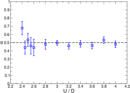
Figure 6: (Color online) Leading exponent $\alpha$ in the behavior of the spectral density $\rho(\omega)$ near the band edges ($\omega\to\Delta$) for various values of $U$. The dashed line marks the value $\alpha=0.5$ suggested by perturbation theory.Gebhard et al. (2003)

Our results excellently confirm the square-root onset. The agreement is very good for large values of the interaction, i.e., deep in the insulating regime. Closer to the closure of the gap the uncertainties grow.

The outer band edges of the Hubbard bands do not show any sharp decay. Instead, they reveal a smooth drop for $|\omega|\to\infty$ which becomes even smoother as $U$ decreases, similar to the behavior of the metallic solutions, cf. Sec. III.2.

III.1.2 Insulating Gap

The gap $\Delta$ is the characteristic quantity of the insulator. Because of the impossibility to determine it directly from the LB deconvolved spectral density we use the value which is found from the fit (23) with fixed exponent $\alpha=1/2$. We stress that this determination of the gap $\Delta$ does not enter the iterations of the self-consistency cycle, except for the removal of artifacts, see App. B.2. It is done only at the end of the iterations once the solution can be considered to be self-consistent according to the criteria in Sec.  II.3.4. This is in contrast to the Fixed-Energy procedure chosen in Ref. Nishimoto and Jeckelmann, 2004 where the gap enters in the self-consistency explicitly. Again, it is a priori not clear which approach is more advantageous. All we found was that we could not reach stable self-consistency when using extrapolated gaps in the devonvolution.

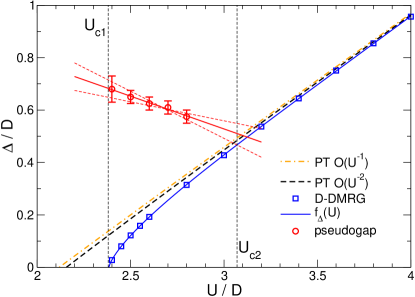
Figure 7: (Color online) Single-particle gap $\Delta$ from the insulating solutions and the pseudogap from the metallic solutions vs. the interaction $U$. The determination of the pseudogap is explained in Sec. III.2. For comparison the results from perturbation theory (PT) up to $\mathcal{O}(U^{-2})$ in the insulating regime are also shown.Eastwood et al. (2003); endnote59

The results are plotted in Fig. 7 as a function of $U$. As expected, the gap $\Delta$ decreases continuously with decreasing $U$ until it vanishes at a critical value $U_{\text{c1}}$. For $U\geq 3.4D$ our $\Delta(U)$ agrees well with the results from perturbation theory expanding in powers of $\nicefrac{{t}}{{U}}$.Eastwood et al. (2003)

Closer to the vanishing gap the behavior of $\Delta(U)$ is not linear anymore but displays a significant curvature. Qualitatively, this is similar to what has been observed previously in iterated perturbation theory Rozenberg et al. (1994) (IPT), by the local moment approachLogan et al. (1997) (LMA), or by the Lanczos approach D-DMRG.García et al. (2004) This observation leads us to fit a power law

$$f_{\Delta}(U)=(U-U_{\text{c1}})^{\zeta}[a_{1}+a_{2}(U-U_{\text{c1}})]$$ (25)

with the fit parameters $a_{i}$, $U_{\text{c1}}$, and $\zeta$, which denotes the leading exponent of $\Delta(U)$ close to $U_{\text{c1}}$. From this fit $U_{\text{c1}}=(2.38\pm 0.02)D$ and $\zeta=0.72\pm 0.05$ is found. Thus, our value for $U_{\text{c1}}$ agrees excellently with most of the previous results, see Tab. 1.

III.1.3 Self-Energy

The self-energy $\Sigma$ is not required in the self-consistency cycle shown in Fig. 2, but it is accessible via Eqs. (3a,6). By means of the self-consistently determined full propagator $G(\omega)$ and the bare propagator $g^{0}(\omega)$ of the SIAM we compute

$$\Sigma(\omega)=\frac{1}{g^{0}(\omega)}-\frac{1}{G(\omega)}.$$ (26)

Note, that this way to access the self-energy can be prone to numerical problems. If the self-energy is a small quantity it can acquire a substantial relative error if it is computed according to (26) as difference of two large quantities. In the extreme case, it can happen that the imaginary part of the retarded self-energy computed via (26) is positive, i.e., it displays the wrong sign and violates causality. This will be a problem in the metallic solutions at weak coupling, see Sec. III.2.

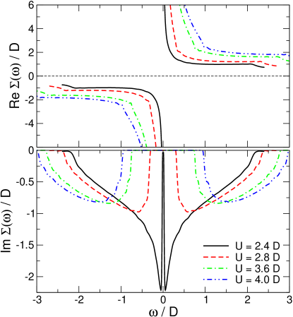
Figure 8: (Color online) Real and imaginary part of the self-energy $\Sigma(\omega)$ in the insulating regime. The $\delta$-peak in the imaginary part (lower panel) is not shown.

The indirectly calculated self-energy in the insulating regime displays the expected features, see Fig. 8. Except for a $\delta$-peak in the imaginary part at $\omega=0$, $\Sigma(\omega)$ is strictly real inside the gap

$$\mathfrak{Im}\,\Sigma(\omega)=-c\pi\delta(\omega)\quad\text{for}\quad|\omega|\leq\Delta\ ,$$ (27)

with $c>0$. Correspondingly, the real part of $\Sigma(\omega)$ shows an $1/\omega$ behavior: $\mathfrak{Re}\,\Sigma(\omega)=c/\omega+\mathcal{O}(\omega)$.

III.1.4 Momentum-Resolved Spectral Densities

So far we discussed the local spectral density $\rho(\omega)$ which is related to the imaginary part of the local propagator $G_{ii}(\omega)$. This is the quantity which matters in the self-consistency of the DMFT approach. But once a self-consistent solution is found one can go a step further towards spatial correlations. While the self-energy and the skeleton diagrams are local in DMFT (see above) one-particle reducible quantities like the propagators are not. Hence it makes sense to discuss $G_{ij}$. Because we study a translationally invariant system we study the propagator in momentum space $G_{k}(\omega)$. Its Dyson equation reads

$$G_{k}(\omega)=\frac{1}{\omega-\epsilon_{k}-\Sigma(\omega)}.$$ (28)

By varying the bare fermionic energy $\epsilon_{k}$ we can assess the effect of different momenta. In particular, if we change $\epsilon_{k}$ from negative to positive values we can view the change of the single-particle response on passing from the dynamics of a hole to the one of an electron.

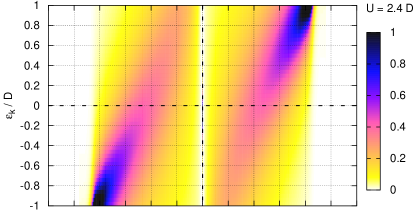
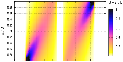
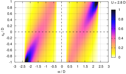
Figure 9: (Color online) Spectral densities $\rho(\omega,\epsilon_{k})$ in the insulating regime for $U=2.4D$ (top), $U=2.6D$ (middle), and $U=2.8D$ (bottom).

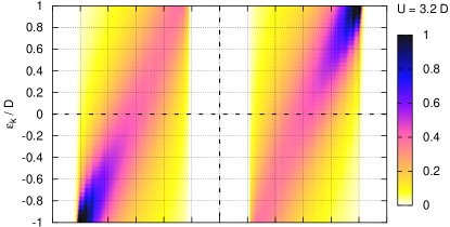
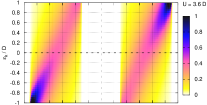
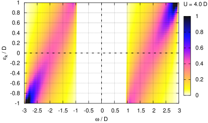
Figure 10: (Color online) Spectral densities $\rho(\omega,\epsilon_{k})$ in the insulating regime for $U=3.2D$ (top), $U=3.6D$ (middle), and $U=4D$ (bottom).

Figs. 9 and 10 display the spectral density of $G_{k}(\omega)$

$$\rho(\omega,\epsilon_{k}):=-\frac{1}{\pi}\mathfrak{Im}G_{k}(\omega).$$ (29)

Tiny wiggles in the intensity as function of the frequency are numerical artifacts of the self-energy computed via (26). The gap between the lower and the upper Hubbard band is clearly visible. In each Hubbard band there is a ridge of high density running from the upper right to the lower left edge. Neglecting the strong scattering we can interpret this ridge as the dispersion of a moving double occupancy in the upper Hubbard band. Correspondingly, there is a moving empty site in the lower Hubbard band. Since the band width of each Hubbard band is approximately equal to the band width of the bare dispersion we deduce that the hopping of the double occupancy or the empty site, respectively, equals the bare hopping. This fact has been exploited also in the perturbative treatment.Eastwood et al. (2003)

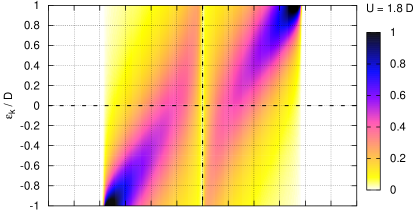
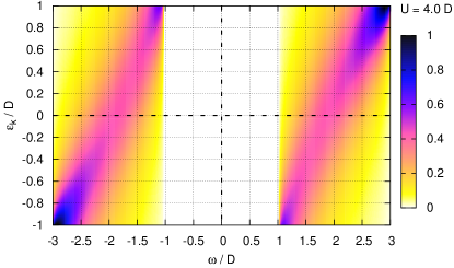
Figure 11: (Color online) Spectral densities $\rho(\omega,\epsilon_{k})$ in the insulating regime according to Hubbard’s approximation in Ref. Hubbard, 1964 for $U=1.8D$ (upper panel) and $U=4.0D$ (lower panel)

Note, that the first approximation to this problem obtained by Hubbard Hubbard (1963) yields only half the band width for each Hubbard band. But the famous improved solution in Hubbard’s third paper Hubbard (1964) displays the correct band width for strong coupling. This treatment also includes scattering processes which take the strong scattering of the additional fermion into account. Hence it is very instructive to compare our numerically exact result with the approximate solution in Ref. Hubbard, 1964. Fig. 11 shows two examples for an almost vanishing gap at $U=1.8D$ and for a large gap at $U=4.0D$. The similarity to the exact results in Fig. 9, upper panel, and in Fig. 10, lower panel, is striking. Both results, exact and approximate, show strongly scattered, hence broadened, excitations in the Hubbard bands. The ridges behave very similarly in shape and height. In particular for the large gap the results agree well.

For the smaller value of the insulating gap, the most important difference is that the value of $U$ differs. But if we accept that the interaction value in Hubbard’s approximation needs to be renormalized in a certain way the spectral densities behave qualitatively very similar. It must be stressed, however, that the results are quantitatively different. Comparing the upper left panel in Fig. 4 with the corresponding result in Ref. Hubbard, 1964 one notes that the spectral weight in the exact solution is found further away from the Fermi level at $\omega=0$ while in Hubbard’s solution it is shifted towards $\omega=0$.

III.2 Metal

III.2.1 Local Spectral Densities

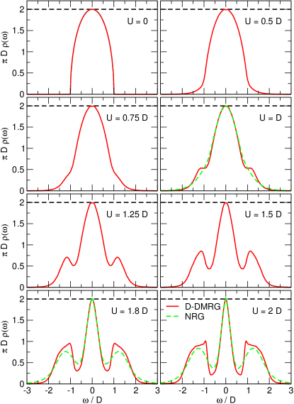
Figure 12: (Color online) Spectral densities $\rho(\omega)$ in the metallic regime calculated with a chain of 160 fermionic sites. The dashed lines show results of a DMFT approach based on the numerical renormalization group (NRG) as impurity solver.Bulla (2004)

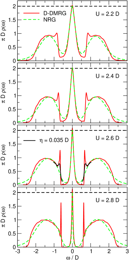
Figure 13: (Color online) Spectral densities $\rho(\omega)$ in the metallic regime close to the metal-to-insulator transition. The dashed lines show results of an NRG-based DMFT approach.Bulla (2004) For $U=2.6D$, the dark solid lines show the raw D-DMRG data broadened with $\eta=0.035D$ around the inner Hubbard band edges, for discussion see Sec. III.2.2

Figure 12 shows the self-consistently calculated spectral densities $\rho(\omega)$ well in the metallic regime ($0\leq U\leq 2D$). Figure 13 shows the corresponding densities $\rho(\omega)$ closer to the transition to the insulating solution at $U=U_{\text{c2}}\approx 3.0D$. We used $160$ fermionic sites (including one site representing the impurity) in the D-DMRG impurity solver. This implies a tiny bias towards the metallic solution, see Sec. II.3.5. The raw data is obtained on an equidistant frequency grid with step size $\Delta\omega_{i}=0.1D$ using a constant broadening $\eta=0.1D$. It is deconvolved using the LB algorithm.Raas and Uhrig (2005) The spectral densities in Figs. 12 and 13 qualitatively display many of the features known from previous analytical Eastwood et al. (2003); Gebhard et al. (2003) and numerical Georges and Kotliar (1992b); Jarrell (1992); Rozenberg et al. (1992); Georges and Krauth (1993); Caffarel and Krauth (1994); Sakai and Kuramoto (1994); Bulla (1999); Bulla et al. (2001); García et al. (2004) investigations.

Starting from the semi-elliptic DOS (7) at $U=0$ the central peak becomes narrower and narrower on increasing $U$. The diminishing width is the Kondo energy scale $T_{\text{K}}$. The weight in the central peak is the quasiparticle weight $Z$ which we will discuss below.

The height of the central peak does not change. The quasiparticle peak is pinned at the Fermi energy to its non-interacting value

$$\rho(\omega=0)=\rho^{0}(\omega=0)=\frac{2}{\pi D}$$ (30)

as required by Luttinger’s theorem for a momentum independent self-energy.Müller-Hartmann (1989) As the DOS at zero frequency is not pre-determined in our approach, the pinning criterion (30) provides a sensitive check for the accuracy of the numerical solutions in the metallic regime. This criterion is very well satisfied, see Fig. 12 and the upper panels in Fig. 13. A maximum relative error of $3\%$ occurs for interaction values close to the transition to the insulator, see lower panels in Fig. 13. The fulfillment of the pinning is an important prerequisite for an accurate determination of the quasiparticle weight $Z$ below.

Beyond $U\approx D$, the DOS shows side features. They are just shoulders which develop into the lower and upper Hubbard bands at larger interaction. As expected, they appear roughly at $\omega=\pm\nicefrac{{U}}{{2}}$. At $U\approx 2D$ the Hubbard bands are well separated from the quasiparticle peak by a precursor of the gap $\Delta$ in the insulator: a pseudogap is formed. This pseudogap is determined from $U=2.4D$ onwards by background fits as shown in Fig. 17. The resulting values and their uncertainties are included in Fig. 7. Their extrapolation corroborates that the pseudogap evolves continuously to the insulating gap at $U_{\text{c2}}\approx 3D$ where the metallic solution becomes unstable towards the insulating solution.

The well pronounced pseudogap in the metallic solutions close to the transition reveals clearly that the quasiparticle peak becomes isolated from the Hubbard bands at higher energies. We demonstrated in Fig. 2 in Ref. Karski et al., 2005 that the spectral densities of the metallic and of the co-existing insulating solution almost coincide at higher energies. This means that except for the quasiparticle peak and the inner edges of the Hubbard bands the insulating and the metallic solutions are almost identical. The two phases differ in their behavior at small and intermediate energies. This phenomenon has been baptized separation of energy scales. The assumption of its validity is at the basis of the numerical projective self-consistent method Moeller et al. (1995); Georges et al. (1996) and of Kotliar’s analytical Landau theory.Kotliar (1999) Hence, the fact that our all-numerical treatment indeed displays the separation of energy scales represents a valuable confirmation of this important hypothesis.

It is very instructive to compare our findings for $\rho(\omega)$ with the NRG data from Ref. Bulla, 2004. The quantitative comparison is depicted in some of the panels in Fig. 12 and in Fig.  13. The agreement is very good in the close vicinity of the quasiparticle peak, i.e., at low energies. But significant deviations are discernible for intermediate and higher frequencies. The Hubbard bands obtained by the D-DMRG are sharper compared to the NRG results. Hence their precursors become visible already at lower values of $U$, see Fig. 12. Furthermore, the Hubbard bands in D-DMRG do not have significant tails at higher energies. This difference stems from the broadening proportional to the frequency which is inherent to the NRG algorithm.Sakai et al. (1989); Costi and Hewson (1990); Bulla (1999); Bulla et al. (2001); Raas et al. (2004) Similar differences were also reported in Ref. Gebhard et al., 2003 where perturbative results are compared with NRG data.

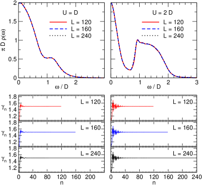
Figure 14: (Color online) Part of the spectral density $\rho(\omega)$ and the associated bath parameters $\gamma_{n}$ calculated self-consistently for various numbers $L$ of fermionic sites. Left panel: $U=D$. Right panel: $U=2D$.

In order to investigate a possible influence of finite-size effects, we consider the self-consistent spectral densities and the associated bath parameters $\gamma_{n}$, cf. Eq. (14), for various sizes of the bath. Fig. 14 shows the results for $L=120$, $160$ and $240$ fermionic sites well in the metallic regime for $U=D$ and $U=2D$. If the finite broadening of the D-DMRG raw data is chosen according to Eq. (19) the spectral densities deconvolved by LB are not affected significantly by the number of bath sites. We observe neither qualitative nor significant quantitative differences. This observation applies also to the self-consistently determined bath parameters $\gamma_{n}$. Above $n\approx 80$ almost all bath parameters take the same value which determines the band width, see App. A.

We conclude that a system size of $80$ fermionic sites is already sufficient to capture quantitatively the features of the spectral properties well in the metallic regime. Nevertheless, a small improvement in the pinning criterion can be observed if more fermionic sites are considered, see Ref. Karski, 2004). This improvement arises from a better approximation of the thermodynamic limit which makes the deconvolution using the LB algorithm more robust. But the system size cannot be chosen too large in practice because the D-DMRG calculation will acquire systematic errors for large systems and given computational resources. Our D-DMRG calculations were all done with 128 states, partly checked by runs with 256 states. But we have not noticed significant deviations between the runs with 128 and those with 256 states.

III.2.2 Sharp Inner Side Peaks

For strong interactions ($U>2D$) close to the metal-to-insulator transition the metallic solutions show sharp peaks at the inner edges of the Hubbard bands, see Fig. 12 for $U=2D$ and Fig. 13. These peaks become sharper and sharper on increasing the interaction $U$. Note, that their height cannot (and does not) exceed the maximum value of the non-interacting DOS because the interacting DOS is determined from the Dyson equation (4). It implies that $\rho(\omega)$ results from $\rho^{0}(\omega)$ by a shift in frequency due to $\mathfrak{Re}\Sigma$ and by a Lorentzian broadening due to $\mathfrak{Im}\Sigma$ so that $\rho(\omega)$ is bounded by the maximum of $\rho^{0}(\omega)$. The sharp features do not represent diverging singularities.

In order to properly resolve the sharp side peaks as well as the narrow quasiparticle peak, we choose $\Delta\omega_{i}=\eta_{i}=0.05D$ and partially $\Delta\omega_{i}=\eta_{i}=0.025D$ in the relevant frequency regions. Furthermore, we place the computed points of the raw data at the frequency of the maximum of the side peaks.

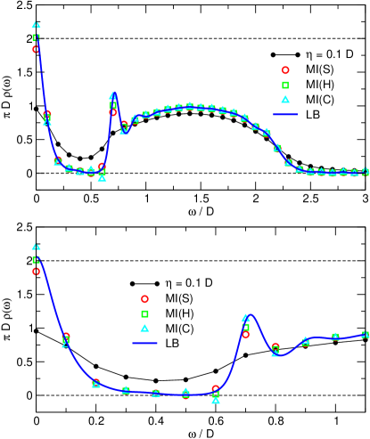
Figure 15: (Color online) Comparison of various deconvolution schemes for $U=2.6D$. The solid line with filled circles depicts the raw data. MI refers to linear matrix inversion for which we assume that the DOS consists of a set of $\delta$-functions [spikes, MI(S): circles] or that it is piecewise constant [histogram, MI(H): squares] or that it is piecewise linear and continuous [MI(C): triangles], for details see Ref. Raas and Uhrig, 2005. LB stands for the continuous positive result obtained by the non-linear LB deconvolution. Upper panel: complete frequency interval of the symmetric DOS. Lower panel: details at lower frequencies.

In Fig. 15 we show that the sharp peaks at the inner band edges are not an artifact of the deconvolution algorithm since a large variety of deconvolution schemes essentially provides the same peak. Furthermore, the side peaks are already discernible in the raw data at small broadening (dark solid lines) shown in Fig. 13 for $U=2.6D$.

We checked that different initial hybridization functions led to the same self-consistent solutions after sufficient iterations so that we exclude that the side peaks are artifacts of the self-consistency procedure. Moreover, Nishimoto et al. found very similar side peaks by a completely independent implementation of DMFT by D-DMRG.Nishimoto et al. (2006) Hence we conclude that the sharp side peaks resolved in our D-DMRG approach are part and parcel of the metallic spectral density of the half-filled Hubbard model close to the metal-to-insulator transition.

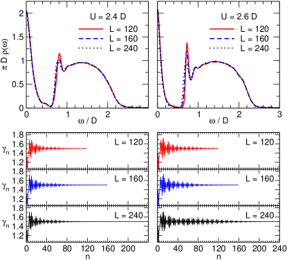
Figure 16: (Color online) Part of the spectral density $\rho(\omega)$ and the associated bath parameters $\gamma_{n}$ calculated self-consistently for various numbers $L$ of fermionic sites. Left: $U=2.4D$. Right: $U=2.6D$.

We repeated the investigation of the possible influence of the system size in Fig. 14 close to the metal-to-insulator transition. In Fig. 16 we compare spectral densities for $U=2.4D$ and $U=2.6D$ and their bath parameters $\gamma_{n}$ determined self-consistently for $120$, $160$, and $240$ fermionic sites with $\Delta\omega_{i}=\eta_{i}=0.1D$. Smaller values for $\Delta\omega$ and $\eta$ turned out not to be feasible for the large system sizes due to limited computational resources. Thus, we accept a slight loss in the resolution of the side peaks compared to the spectral densities shown in Fig. 13 where calculations with $\Delta\omega_{i}=\eta_{i}=0.025D$ were performed for frequencies around the side peak positions.

We see in Fig. 16 that the precise position and the shape of the side peaks depend slightly on the size of the bath considered in the numerical calculations. The other, less sharp features, like the central peak and the Hubbard band are very robust against the changes of the bath size. It is very instructive to look at the bath paramters $\gamma_{n}$. For $U=2.4D$ they do not change on passing from $L=120$ over $L=160$ to $L=240$. The oscillations visible from smaller values of $n\lessapprox 80$ are essentially the same for the three system sizes. They do not extend to larger $n$ for larger $L$. For $U=2.6D$, however, the bath parameter change for larger systems. The oscillations extend to higher $n$ for $L=240$ than for lower $L$. For $L=240$ they appear to have converged for large $n$ so that we assume that increasing $L$ further would only extend the region of almost constant $\gamma_{n}$.

We conclude, that sufficiently large baths are essential for a quantitative description of the spectral densities and of the sharp features at the inner edges of the Hubbard bands in particular. This is especially important close to the metal-to-insulator transition. Our results confirm the existence of the sharp side peaks and provide their accurate determination for all $U\leq 2.2D$. For $U>2.2D$ the possibility of small inaccuracies of the order of the deviations shown in the upper panels of Fig. 16 must be kept in mind.

The only previous evidence for sharp side peaks in numerical investigations were weak shoulders in NRGBulla (1999) and quantum Monte Carlo (QMC)Blümer (2003) data. The inherent broadening in the NRG calculations and the necessity to continue the QMC data from imaginary times to real frequencies have both a tendency to smear out sharp features away from the Fermi level, cf. Ref. Raas et al., 2004. Hence we tend to interprete the shoulders in Refs. Bulla, 1999 and Blümer, 2003 as broadened remnants of the sharp peaks resolved in the present D-DMRG calculation.

Besides the numerical approaches semi-analytical approaches, the iterated perturbation theory (IPT)Georges et al. (1996) and the non-crossing approximation (NCA),Pruschke et al. (1993) display similar behavior of the spectral densities near the inner Hubbard band edges. The IPT results show a substantial accumulation of spectral weight at the inner band edges which differs very much from our findings: the weight is much larger and the features are by far not as sharp as those presented here. They carry even more spectral weight than the quasiparticle peak and they are accompanied by spike structures over the entire Hubbard bands in contrast again to our findings. In view of these differences and because IPT is an approximate diagrammatic approach we conclude that the IPT features do not correspond to the ones presented here.

The NCA data in Ref. Pruschke et al., 1993 is qualitatively much closer to our data as far as the side peaks are concerned. Since the NCA violates the Fermi liquid properties for temperatures lower than the Kondo scale Müller-Hartmann (1984) reliable conclusions can only be drawn for sufficiently large temperatures. Moreover, the peaks are found in the insulating phase so that it is an open question whether the NCA findings are related to the D-DMRG side peaks at zero temperature in the metallic regime.

In order to pave the way to a physical interpretation of the side peaks we determine its weight $S$. Motivated by the results for insulating $\rho(\omega)$ in Sec. III.1.1 we fit an approximate square-root onset multiplied by a quadratic polynomial to the Hubbard band. The excess weight is identified with the spectral weight $S$ of the sharp side peak. This procedure is illustrated in Fig. 17.

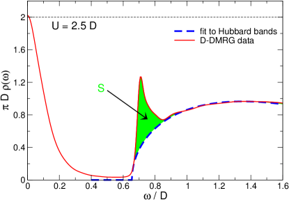
Figure 17: (Color online) Determination of the side peak weight $S$ illustrated for $U=2.5D$.

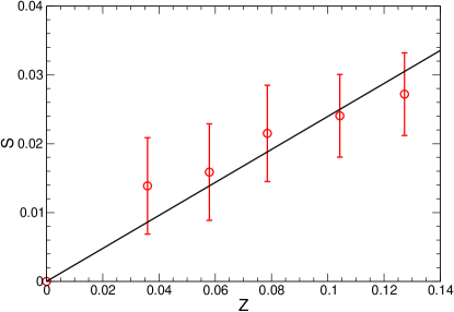
Figure 18: Weight $S$ of the peaks at inner Hubbard band edges as a function of the quasiparticle weight $Z$.

Inspection of Fig. 13 suggests that $S$ vanishes for $U\to U_{\text{c2}}$. This conclusion is supported by the fact that the insulating solutions do not display a similar feature, see Sec. III.1.1. Hence we presume that the side peak involves quasiparticles from the central peak. The weight in this central peak is given by $Z$ which vanishes linearly for $U\to U_{\text{c2}}$, see Sec. III.2.4. So we plot the results for $S$ as function of $Z$ in Fig. 18 including a point $S=0$ for $Z=0$. The error bars result from the numerical difficulty to resolve this sharp feature and from the analytical difficulty to separate it from the background of the Hubbard bands.

In view of the errors the interpretation of Fig. 18 is daring. But our guiding hypothesis is that the surprisingly sharp side peak is the signature of a composite excitation involving several fermionic excitations.Karski et al. (2005) A single quasiparticle alone cannot be at the origin of a sharp feature because it has a finite dispersion and a finite life-time so that it engenders only broad features in local quantities away from the Fermi level.

One possible assumption is that the composite excitation comprises three quasiparticles (Note, that the total statistics must be fermionic.). But they need to be bound or anti-bound to account for the very sharp structure which tells us that the composite entity must be almost immobile. Otherwise it would give rise only to a broad structure in local spectral densities, which correspond to sums over the entire Brillouin zone. A plausible second scenario is that a single quasiparticle is combined with a collective mode, for instance a particle-hole pair as it occurs when a spin is flipped.

With these ideas in mind, we want to use Fig. 18 only to decide whether one, two or three quasiparticles are involved. The quasiparticle weight $Z$ measures to which extent a local fermionic creation operator generates a true quasiparticle including its polarization dressing. So we presume that the contribution of a single quasiparticle gives rise to a linear behavior $S\propto Z$ while two quasiparticles lead to $S\propto Z^{2}$, and three quasiparticles imply $S\propto Z^{3}$. Hence we find in the linear fit in Fig. 18 a hint that only one quasiparticle contributes to the side peaks.

Additionally, we presume that an immobile collective mode is involved. Note, that due to the scaling (2) in DMFT collective modes are as such immobile because their motion requires at least two single-particle propagators. The nature, however, of the collective mode inducing the composite feature is still an open issue which we address in ongoing investigations.

III.2.3 Self-Energy

In the metallic phase we use again Eq. (26) to obtain the self-energy. The results are plotted in Fig. 19. The real and imaginary part of the self-energy display a typical low-frequency behavior of a local Fermi liquid: The real part shows a linear behavior with a negative slope which steepens as $U$ increases. In this region, the imaginary part of $\Sigma(\omega)$ shows a quadratic behavior, $\mathfrak{Im}\,\Sigma(\omega)\propto-\omega^{2}$, as expected.Müller-Hartmann (1989) The quadratic behavior of $\mathfrak{Im}\Sigma$ is not perfectly retrieved, see inset of Fig. 19. For low values of $U$ it seems that $\mathfrak{Im}\Sigma$ is proportional to a higher power than $\omega^{2}$ for $\omega\to 0$. For large interaction values, for instance $U=2.6D$, the computation of the self-energy via (26) even leads to negative spectral densities (positive $\mathfrak{Im}\Sigma$ for the retarded self-energy) violating causality. This is a clear indication for the limits of the accuracy of the present calculation. But we stress that these difficulties are minor and do not affect the self-consistency because they occur only when the self-energy is computed from the full propagator $G$.

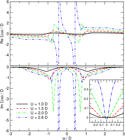
Figure 19: (Color online) Real and imaginary part of the self-energy $\Sigma(\omega)$ in the metallic regime. Inset: $\mathfrak{Im}\,\Sigma(\omega)$ on a larger scale.

The two-peak structure in the imaginary part of $\Sigma(\omega)$ is closely related to the three-peak structure of the spectral density given by lower Hubbard band, central Kondo peak, and the upper Hubbard band. According to Eq. (26) the self-energy has a peak if the real and the imaginary part of $G(\omega)$ are small. For the metallic solutions, this is the case in the frequency regime between the Hubbard bands and the quasiparticle peak, i. e. within the pseudogap.

This relation has been previously analyzed.Zhang et al. (1993); Kehrein (1998); Bulla (1999) It turns out that the strong peaks in the self-energy are located at position $\omega_{\Sigma}\propto\pm\sqrt{Z}D$, where $Z$ is the quasiparticle weight, see next subsection. Our data agrees very well with the analytical arguments; the factor of proportionality is about $\sqrt{2}$. We stress that $\omega_{\Sigma}\to 0$ on approaching the metal-to-insulator transition whereas the sharp inner side peaks remain at the inner band edges. Hence the two peaks in the imaginary part of the self-energy are not directly related to the sharp side peaks. It should be pointed out that the two-peak structure of the self-energy contradicts the findings in Ref. Kehrein, 1998. We presume that the analytical argument misses some effect which requires further research.

III.2.4 Quasiparticle Weight

The quasiparticle weight $Z$ is the characteristic quantity of the metallic phase. Crudely speaking $Z$ quantifies how much of the spectral weight is found in the central quasiparticle peak, cf. Fig. 13 and 12. In other words, $Z$ is the matrix element between the fermionic creation operator applied to the ground-state and the dressed quasiparticle excitation including its polarization cloud. For local self-energies Müller-Hartmann (1989) it is given by

$$Z^{-1}=1-\left.\partial_{\omega}\Sigma(\omega)\right|_{\omega=0}.$$ (31)

Because the self-energy is not directly accessible in our approach we prefer to calculate $Z$ using the derivative of the Dyson equation (4) implying

$$Z^{-1}=\frac{D^{2}}{2}\left.\partial_{\omega}G(\omega)\right|_{\omega=0},$$ (32)

where $\partial_{\omega}G^{0}(\omega)|_{\omega=0}=\nicefrac{{2}}{{D^{2}}}$ has been used. By Eq. (32) we avoid the numerical errors occurring if the self-energy is determined via (26), see Sec. III.2.3.

The derivative $\partial_{\omega}G(\omega)|_{\omega=0}$ in Eq. (32) is real because the imaginary part displays an extremum at $\omega=0$. The derivative of $\mathfrak{Re}\,G(\omega)$ is obtained reliably from the coefficient $a$ of the fit function

$$f_{\mathfrak{Re}\,G}(\omega)=a\omega+b\omega^{3}$$ (33)

where the absence of even orders due to particle-hole symmetry has been taken into account. The fit is done in the intervals around the origin which decrease for $U\to U_{\text{c2}}$ roughly linearly; for $U=2D$ it is $[-0.1D,0.1D]$. The derivative cannot be determined robustly as ratio of differences because $\mathfrak{Re}\,G(\omega)$ displays weak oscillations resulting via the Kramers-Kronig transformation from weak wiggles in $\mathfrak{Im}\,G(\omega)$ due to the deconvolution procedure, see for instance the lowest panel in Fig. 13 around $\omega=D$.

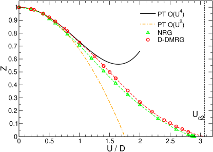
Figure 20: (Color online) Quasiparticle weight $Z$ as a function of $U$ compared to perturbative resultsGebhard et al. (2003) (PT) up to $\mathcal{O}(U^{4})$ and to NRG data.Bulla (1999)

In Fig. 20 the quasiparticle weight $Z$ is depicted as a function of $U$. Starting from $Z=1$ at $U=0$, $Z$ decays as $U$ increases. Our results agree excellently with perturbation theory where it is applicable $U\lessapprox D$. The NRG data is lower for all values of $U$. We deduce that the broadening of the spectral weights proportional to $\omega$, inherent to NRG, has a non-negligible influence on the quasiparticle weight. Qualitatively, however, the behavior of $Z(U)$ is very similar.

From the trend of $Z(U)$ one expects that $Z$ vanishes continuously at a finite critical value $U_{\text{c2}}$. We cannot approach this value arbitrarily closely because the reliable resolution of the sharper and sharper quasiparticle peak would require a better and better resolution. This in turn cannot be achieved with a reasonable amount of computing resources because Eq. 19 must be respected. For this reason, we have to resort to an extrapolation to determine $U_{\text{c2}}$ quantitatively.

The behavior of $Z(U)$ close to $U_{\text{c2}}$ was already investigated previously analytically by the projected self-consistent method (PSCM) Moeller et al. (1995) and by the linearized DMFT.Bulla and Potthoff (2000) Both methods assume the separation of energy scales and predict a linear behavior of $Z$ close to $U_{\text{c2}}$. Since our all-numerical spectral densities strikingly confirm the separation of the energy scales Karski et al. (2005) we determine $U_{\text{c2}}$ by fitting

$$f_{Z}(U)=a_{1}(U-U_{\text{c2}})+a_{2}(U-U_{\text{c2}})^{2}$$ (34)

to the data points for $U\in[2,\,2.8]D$. We obtain a critical value of $U_{\text{c2}}=(3.07\pm 0.1)D$ which agrees excellently within the error range with most of the previous results,Moeller et al. (1995); Bulla (1999); Bulla and Potthoff (2000); Bulla et al. (2001); García et al. (2004); Blümer and Kalinowski (2005, 2005) including the linearized DMFTBulla and Potthoff (2000) and the PSCM.Moeller et al. (1995) For comparison, we include an overview of these critical values in Tab. 1.

$U_{\text{c1}}$/D	$U_{\text{c2}}$/D	method
$2.38\pm 0.02$	$3.07\pm 0.1$	D-DMRG (CV, direct inversion)
$2.225\pm 0.025$	$3.05\pm 0.05$	D-DMRG (CV, variational)Nishimoto et al. (2004, 2006)
$2.39\pm 0.02$	$3.0\pm 0.2$	D-DMRG (Lanczos)García et al. (2004)
$2.39$		PT-QMCBlümer and Kalinowski (2005)
$2.39$	$2.94$	NRGBulla (1999); Bulla et al. (2001)
	$3$	linearized DMFTBulla and Potthoff (2000)
	$2.92\pm 0.05$	PSCMMoeller et al. (1995)

Table 1: Comparison of the values for $U_{\text{c1}}$ and $U_{\text{c2}}$ found by various approaches.

III.2.5 Momentum-Resolved Spectral Densities

For the metallic phase, we present spectral densities $\rho(\omega,\epsilon_{k})$ as defined in Eqs. (28,29) which are resolved according to their bare single-particle energy $\epsilon_{k}$. In the context of the DMFT, this procedure provides information on the momentum dependence of the spectral properties. Figs. 21 and 22 display how the momentum-resolved spectral densities evolve on approaching the metal-to-insulator transition.

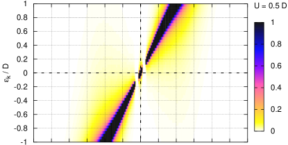
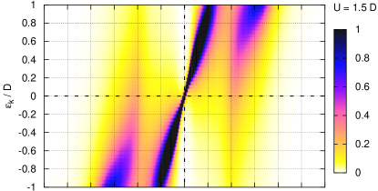
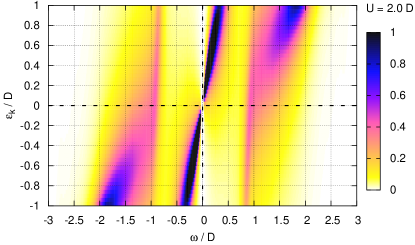
Figure 21: (Color online) Spectral densities $\rho(\omega,\epsilon_{k})$ in the metallic regime for $U=0.5D$ (top), $U=D$ (middle), and $U=2D$ (bottom).

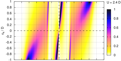
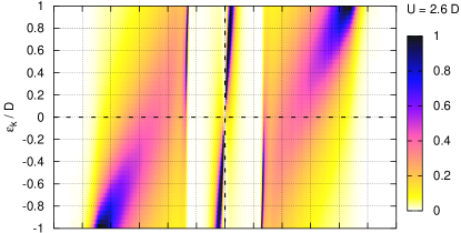
Figure 22: (Color online) Spectral densities $\rho(\omega,\epsilon_{k})$ in the metallic regime for $U=2.4D$ (top), $U=2.6D$ (middle), and $U=2.8D$ (bottom).

Three main features can be discerned. First, the dominant diagonal line of highest intensity with $\omega_{\text{high}}\propto\epsilon_{k}$ catches our attention in all six panels. This is where the Fermi liquid picture manifests itself.Nozières (1997) Without interaction a quasiparticle can be excited at $\omega_{\text{high}}=\epsilon_{k}$. In the presence of interaction there are still quasiparticles which behave like fermions above the Fermi level or holes below it. But these excitations are dressed by clouds of particle-hole pairs. This dressing has two effects. One is that the bare fermionic operator has only an overlap reduced by $Z$ with the creation of the quasiparticle. The other effect is that the dressed quasiparticles are heavier than their bare counterparts. This means that their dispersion is reduced. For a momentum-independent self-energy the reduction of the dispersion is given again by the factor $Z\leq 1$. This can be seen in the impressive steepening of the dominant diagonal line given by $\omega_{\text{high}}=Z\epsilon_{k}$ upon increasing interaction. For interaction values close to the instability of the metallic solution, see lowest panel in Fig. 22, the diagonal line has become so steep that it can almost be taken as a vertical one. This implies that the quasiparticle has become almost local and non-dispersive. This is the mechanism leading to the so-called heavy fermions.

We point out that the white stripes at $\omega=0$ in most of the panels in Figs. 21 and 22 and the white stripes at small $\omega$ in the first panel of Fig. 21 result from the numerical violations of causality as discussed before, see Sects. III.1.3 and III.2.3. For values of $\omega$ where this problem occurs the spectral densities are set to zero.

The second main feature in the momentum-resolved spectral densities is the development of the precursors of the lower and the upper Hubbard band. At $U=0.5D$ no such precursors are visible, except for some broadening of the diagonal line away from the Fermi level. But in the panel for $U=1.5D$ the precursors are already clearly visible. They are qualitatively very similar to the broad densities found in the insulating spectral densities in Figs. 9 and 10. This similarity becomes more and more pronounced as $U$ approaches $U_{\text{c2}}$ where the metal changes continuously to the insulator.

The third main feature is the occurrence of a vertical line of high density at the inner edges of the precursors of the Hubbard bands. It is barely visible for $U=2.0D$, see last panel of Fig. 21. But it is clearly discernible for the larger values of the interaction displayed in Fig. 22. This vertical line represents the momentum-resolved feature of the sharp side peaks at the inner band edges discussed in Sec. III.2.2. We re-emphasize that there is no discernible momentum dependence indicating a local, non-dispersive, immobile excitation.

We draw the reader’s attention to the fact that the vertical lines display an interesting dependence of their weight on the momentum. The high density is found for $\omega>0$ for $\epsilon_{k}<0$ and vice versa ($\omega<0$ for $\epsilon_{k}>0$). This implies that the immobile composite entity is excited upon adding a bare fermion ($\omega>0$), but for momenta corresponding to occupied states ($\epsilon_{k}<0$) and vice versa. We deduce that the addition of the bare fermion must induce the creation of a quasiparticle hole, cf. Sec. III.2.2. Further work to elucidate this puzzling behavior is called for.

IV Summary

The present work constitutes the comprehensive analysis of the transition from a metal to an insulator driven by strong repulsive interaction. The framework of this investigation is the dynamic mean-field theory (DMFT). We evaluate the necessary self-consistency equations at zero temperature with a numerical impurity solver based on dynamic density-matrix renormalization (D-DMRG). The D-DMRG computes a frequency-dependent correction vector which ensures a high reliability of the results at all energies, not only close to the Fermi level. Thereby, we are able to provide spectral densities in the metallic and in the insulating phase with unprecedented resolution. Such densities are relevant to photoelectron spectroscopy of transition metal compounds and other narrow-band systems.

The calculations are done for a semi-elliptic non-interacting density of states (DOS). All the important technical details of the intricate combination of D-DMRG and DMFT are given in detail so that our findings may be reproduced independently.

The local, momentum-integrated, spectral density in the insulating phase is governed by the lower and the upper Hubbard band. Both are featureless and display square-root singularities at the inner band edges. The insulating gap $\Delta$ vanishes continuously for $U\to U_{\text{c1}}=(2.38\pm 0.02)D$. A slight curvature indicates that $\Delta\propto(U-U_{\text{c1}})^{\zeta}$ with $\zeta=0.72\pm 0.05$.

For $U<U_{\text{c2}}=(3.07\pm 0.1)D$ the insulating solution is only metastable. The phase with lower ground-state energy is the metallic one.Karski et al. (2005) The corresponding spectral densities show three important features for significant interaction values: (i) the central quasiparticle peak, (ii) the precursors of the lower and the upper Hubbard band, and (iii) the sharp side peaks at the inner band edges of the Hubbard bands.

The DOS of the central peak at the Fermi level is pinned to its non-interacting value due to Luttinger’s theorem. The central peak is built from heavy fermions or holes which disperse only weakly due to their strong dressing. They are the characteristic signature of a Fermi liquid.

The Hubbard bands signal that the metal evolves towards an insulator on increasing interaction. Our findings, both the earlier ones Karski et al. (2005) and the present ones, clearly show that the metallic spectral densities evolve continuously to the insulating one upon $U\to U_{\text{c2}}$. This continuity holds in the sense of an integral norm, i.e., considering the distribution of spectral weight, not in the sense of an absolute value norm which jumps. For instance, the DOS at the Fermi level is $2/(\pi D)$ in the metallic regime and zero in the insulating one. But the corresponding weight vanishes linearly for $U\to U_{\text{c2}}$. The pseudogap develops simultaneously to the insulating gap. These findings numerically confirm the assumption of the separation of energy scales.Moeller et al. (1995); Kotliar (1999)

The sharp side peak at the inner edges of the Hubbard bands in the metallic regime are the signature of a complex composite excitation which is not yet understood. We found that its weight scales with the quasiparticle weight which supports our hypothesis that the side peaks stem from an entity made from a quasiparticle and some collective, immobile mode. The analysis of the momentum-resolved spectral densities shows in addition that the involved quasiparticle is a hole if a bare electron is added. Conversely, it is a particle if a bare hole is created, i.e., an electron is taken out.

Ongoing research is devoted to the nature of the composite excitation which generates the sharp side peaks. To this end, the response functions, which correspond to various collective modes, need to be investigated.

Other interesting issues concern the qualitative and quantitative dependence of the important features found on the non-interacting density of states. The changes introduced by doping certainly will be of particular interest. A first study, based on Lanczos-DMRG, of the effects of doping has been published very recently.Garcia et al. (2007)

Appendix A Calculation of the Continued Fraction Coefficients

Once a propagator $g(\omega)$ is known on a dense mesh of frequencies (about $10^{5}$ points), one is able to determine its continued fraction representation to an arbitrary depth

$$g(\omega)=\cfrac{{b}_{0}^{2}}{\omega-a_{0}-\cfrac{b_{1}^{2}}{\omega-a_{1}-\cfrac{b_{2}^{2}}{\omega-a_{2}-\cdots}}}$$ (35)

very precisely. Numerically, only integrations are involved.

For the iteration, we define recursively the resolvents

$$p_{0}(\omega) :=g(\omega)\ ,$$ (36a)

$$p_{n+1}(\omega) =\omega-a_{n}-\frac{b_{n}^{2}}{p_{n}(\omega)}.$$ (36b)

Obviously, the continued fraction representation of $p_{n}(\omega)$ starts with $a_{n}$ and $b_{n}$. It is shifted by $n$ relative to the continued fraction of $g$. An expansion in $1/\omega$ reads

$$p_{n}(\omega)=\frac{b_{n}^{2}}{\omega}\left(1+\frac{a_{n}}{\omega}+\mathcal{O}(\omega^{-2})\right).$$ (37)

Comparing this expression with the expansion in $1/\omega$ of the Hilbert representation of $p_{n}(\omega)$ Pettifor and Weaire (1985); Viswanath and Müller (1994) leads to

$$b_{n}^{2} =-\frac{1}{\pi}\int\limits_{-\infty}^{\infty}\mathrm{d}\omega\,\mathfrak{Im}\,p_{n}(\omega)\ ,$$ (38a)

$$a_{n} =-\frac{1}{\pi b_{n}^{2}}\int\limits_{-\infty}^{\infty}\mathrm{d}\omega\,\omega\,\mathfrak{Im}\,p_{n}(\omega).$$ (38b)

The iteration of the above equations for $n=0,1,2,\ldots$ yields the wanted coefficients. The iterations are stopped once all the coefficients for the numerically tractable finite chain of $L$ fermionic sites are determined, i.e., for $n=L-3$.

In the case of a particle-hole symmetric model, the spectral density is symmetric. Consequently, all odd moments and thus all the coefficients $a_{n}$ ($n=0,1,\ldots$) vanish in the above recursion scheme. So for the model under study we need only to consider the equations for the $b_{n}$.

The asymptotic behavior of the continued fraction coefficients for $n\to\infty$ is determined by the band width of the spectral density $\rho(\omega)$ and by the singularities at the band edges. Pettifor and Weaire (1985); Viswanath and Müller (1994) We exploit the relation for the band width $2B$, if the support of the spectral density is compact, which reads

$$4|b_{\infty}|=2B$$ (39)

where $b_{\infty}:=\lim_{i\to\infty}b_{i}$. For a gap $\Delta$ in the middle of the spectral density, i.e., for the insulator, the $b_{i}$ are oscillating for large $i$ like

$$b_{i}\to b_{\infty}\pm(-1)^{i}\Delta/2$$ (40)

where $b_{\infty}$ is again given by a quarter of the band width which is the distance between the largest and the smallest band edge including the gap.

In a strict sense we expect that the support of the spectral density of an interacting system is infinitely large. But it turns out that significant spectral weight is found only in a finite interval. The contributions outside this interval are negligible which has been observed also in other calculations. Eastwood et al. (2003)

We use the relations (39,40) to determine the interval in which we have to compute raw data $\{g_{i}\}$. For this purpose we compute $b_{\infty}$ in each iteration of the self-consistency cycle and observe its development on iteration. If the value of $b_{\infty}$ does not change significantly for several iteration steps, we fix the border $B$ of the interval in which we perform the calculation of the raw data. This procedure allows us to avoid the time-consuming calculation of unnecessary data points.

In the presence of an insulating gap $\Delta$ at the Fermi energy the above recursion scheme (38) to determine the continued fraction coefficients has to be modified for practical reasons. Due to the antisymmetry of its real part the propagator in the particle-hole symmetric case vanishes at $\omega=0$ completely $p_{0}(\omega=0)=0$ with no imaginary part. So there is a pole in $p_{1}(\omega)$ at $\omega=0$ according to (36b) implying a finite contribution from a $\delta$-distribution at $\omega=0$ in $\mathfrak{Im}\,p_{1}$. We account for it separately

$$\begin{split}b_{1}^{2}&=-\frac{1}{\pi}\int\limits_{-\infty}^{\infty}\mathrm{d}\omega\,\mathfrak{Im}\,p_{1}(\omega)\\ &=-\frac{1}{\pi}\int\limits_{\mathbb{R}\setminus[-\Delta,\Delta]}\mathrm{d}\omega\,\mathfrak{Im}\,p_{1}(\omega)+\frac{b_{0}^{2}}{|p^{\prime}_{0}(0)|}.\end{split}$$ (41)

The recursion relation (36b) implies that the same scenario occurs for every odd $n$. So we use (41) for any odd $n$ once the subscript ₁ is replaced by _n and the subscript ₀ by _n-1.

Appendix B Removal of Deconvolution Artifacts

B.1 Outer Band Edges

The raw data $\{g_{i}\}$ from D-DMRG covers only a certain finite interval. Hence the underlying unbroadened spectral density $\rho(\omega)$ can also be determined only on a finite interval $[-B,B]$ ($B\approx 3D$) which is very close to the interval in which the raw data is available. The deconvolution leads to an abrupt increase of the deconvolved $\rho(\omega)$ at the assumed band edges at $B$, see Fig. 23. This increase is definitely an artifact. In general, we expect that the spectral density $\rho(\omega)$ continues to decrease for $|\omega|\to\infty$. This decrease is a gradual one, i.e., there is no band edge in the strict sense for the correlated system. But all results obtained so far by us and others Eastwood et al. (2003) point into the direction that the contributions beyond a certain interval can be safely neglected.

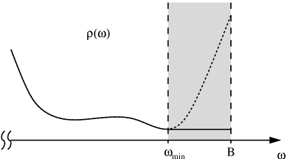
Figure 23: Lines: Generic deconvolved spectral density close to the band edge at $B$. The dashed line marks the artifact which is removed by setting $\rho(\omega>\omega_{\text{min}})=\rho(\omega_{\text{min}})$. The left band edge is treated accordingly.

The artificial increase is removed by replacing $\rho(\omega)$ for frequencies beyond $\omega_{\text{min}}$ where the first minimum occurs by the minimal value $\rho(\omega_{\text{min}})$. This is indicated by the dashed line in Fig. 23 which is replaced by the solid curve.

B.2 Inner Band Edges of the Insulator

The situation close to inner band edges stemming from a gap is similar to the one close to outer band edges. The LB deconvolution of the D-DMRG raw data in the region, where the insulating solution displays a gap, leads to small artifacts as shown in Fig. 24 by the dashed lines.

Figure 24: Lines: Generic deconvolved spectral density in the region of the gap $\Delta$ of the insulating phase. The dashed line marks the artifacts which are cut out by setting $\rho(\omega)$ to zero for $\omega\in[-\Delta_{\delta},\Delta_{\delta}]$.

The first remedy, which one may consider, is to determine the gap $\Delta^{\text{stat}}$ of the SIAM by conventional static DMRG and to use this value as the gap of the lattice problem in DMFT. But we found out that even an extrapolation of this static gap $\Delta^{\text{stat}}$ to the thermodynamic limit $L\to\infty$, as proposed in Ref. Nishimoto et al., 2004, cannot be used in our iterations. No stable self-consistent solution in the sense of the criteria given in Sec. II.3.4 could be obtained.

The successful treatment of the artifacts consisted in removing only the obviously artificial features which are depicted by dashed lines in Fig. 24. The solid lines are kept because they represent real spectral weight. This is done by starting from the value of the static gap $\Delta^{\text{stat}}$ adjusted by a correction parameter $\delta>0$

$$\rho(\omega)\equiv 0\quad\forall\omega\in[-\Delta^{\text{stat}}+\delta,\,\Delta^{\text{stat}}-\delta].$$ (42)

The value $\delta$ is chosen carefully, so that on the one hand all deconvolution artifacts are removed and on the other hand the proper spectral weight of the Hubbard bands stays untouched. In order to determine the appropriate value of $\delta$ it is helpful to resolve the inner Hubbard band-edges in detail, which can be achieved by small values of $\eta_{i}$ in this region. Note, that the adjusted interval $[-\Delta^{\text{stat}}+\delta,\,\Delta^{\text{stat}}-\delta]$ can be set smaller than the interval $[-\Delta,\Delta]$ defined by the proper gap $\Delta$ as long as all deconvolution artifacts are removed. The artifacts would spoil the DMFT self-consistency iteration because the continued fraction coefficients could not be evaluated properly.

It turns out that $\delta$ does not need to be changed in each iteration of the DMFT self-consistency cycle. It is sufficient to set it once for each value of $U$.

References

- Metzner and Vollhardt (1989) W. Metzner and D. Vollhardt, Phys. Rev. Lett. 62, 324 (1989).
- Müller-Hartmann (1989) E. Müller-Hartmann, Z. Phys. B 74, 507 (1989).
- Georges and Kotliar (1992a) A. Georges and G. Kotliar, Phys. Rev. B 45, 6479 (1992a).
- Jarrell (1992) M. Jarrell, Phys. Rev. Lett. 69, 168 (1992).
- White (1992) S. R. White, Phys. Rev. Lett. 69, 2863 (1992).
- White (1993) S. R. White, Phys. Rev. B 48, 10345 (1993).
- Ramasesha et al. (1997) S. Ramasesha, S. K. Pati, H. R. Krishna-murthy, Z. Shuai, and J. L. Brédas, Synthetic Metals 85, 1019 (1997).
- Kühner and White (1999) T. D. Kühner and S. R. White, Phys. Rev. B 60, 335 (1999).
- Raas et al. (2004) C. Raas, G. S. Uhrig, and F. B. Anders, Phys. Rev. B 69, 041102(R) (2004).
- Karski et al. (2005) M. Karski, C. Raas, and G. S. Uhrig, Phys. Rev. B 72, 113110 (2005).
- Kanamori (1959) J. Kanamori, J. Phys. Chem. Solids 10, 87 (1959).
- Hubbard (1963) J. Hubbard, Proc. R. Soc. London 276, 238 (1963).
- Gutzwiller (1963) M. C. Gutzwiller, Phys. Rev. Lett. 10, 159 (1963).
- Kotliar (1999) G. Kotliar, Eur. Phys. J. B 11, 27 (1999).
- Karski (2004) M. Karski, Dynamische Molekularfeldtheorie mittels dynamischer Dichtematrix-Renormierung (Diplomarbeit, Universität zu Köln, 2004), available at http://t1.physik.uni-dortmund.de/uhrig/.
- Potthoff (2003) M. Potthoff, Eur. Phys. J. B 36, 335 (2003).
- Uhrig (1996) G. S. Uhrig, Phys. Rev. Lett. 77, 3629 (1996).
- Georges et al. (1996) A. Georges, G. Kotliar, W. Krauth, and M. J. Rozenberg, Rev. Mod. Phys. 68, 13 (1996).
- Economou (1979) E. N. Economou, Green’s Functions in Quantum Physics, vol. 7 of Solid State Sciences (Springer, Berlin, 1979).
- Pettifor and Weaire (1985) D. G. Pettifor and D. L. Weaire, The Recursion Method and Its Applications, vol. 58 of Springer Series in Solid-State Sciences (D. G. Pettifor and D. L. Weaire, Berlin, 1985).
- Hewson (1993) A. C. Hewson, The Kondo Problem to Heavy Fermions (Cambridge University Press, Cambridge, 1993).
- Hallberg (1995) K. A. Hallberg, Phys. Rev. B 52, R9827 (1995).
- Raas and Uhrig (2005) C. Raas and G. S. Uhrig, Eur. Phys. J. B 45, 293 (2005).
- Hövelborn (2000) T. Hövelborn, Boundary Dynamics of the XY-Chain with the Density Matrix Renormalization Group (Diplomarbeit, Universität zu Köln, Universität Bonn, 2000), available at http://t1.physik.uni-dortmund.de/uhrig/.
- Raas (2005) C. Raas, Ph.D. thesis, Universität zu Köln (2005), available at http://www.raas.de/.
- Press et al. (1992) W. H. Press, S. A. Teukolsky, W. T. Vetterling, and B. P. Flannery, Numerical Recipes (Cambridge University Press, Cambridge, 1992).
- Nishimoto et al. (2004) S. Nishimoto, F. Gebhard, and E. Jeckelmann, J. Phys.: Condens. Matter 16, 7063 (2004).
- Nishimoto et al. (2006) S. Nishimoto, F. Gebhard, and E. Jeckelmann, Physica B 378-380, 283 (2006).
- Eastwood et al. (2003) M. P. Eastwood, F. Gebhard, E. Kalinowski, S. Nishimoto, and R. M. Noack, Eur. Phys. J. B 35, 155 (2003).
- Jeckelmann (2002) E. Jeckelmann, Phys. Rev. B 66, 045114 (2002).
- Viswanath and Müller (1994) V. S. Viswanath and G. Müller, eds., The Recursion Method; Application to Many-Body Dynamics, vol. m23 of Lecture Notes in Physics (Springer, Berlin, 1994).
- Gebhard et al. (2003) F. Gebhard, E. Jeckelmann, S. Mahlert, S. Nishimoto, and R. M. Noack, Eur. Phys. J. B 36, 491 (2003).
- García et al. (2004) D. J. García, K. Hallberg, and M. J. Rozenberg, Phys. Rev. Lett. 93, 246403 (2004).
- Nishimoto and Jeckelmann (2004) S. Nishimoto and E. Jeckelmann, J. Phys.: Condens. Matter 16, 613 (2004).
- Blümer and Kalinowski (2005) N. Blümer and E. Kalinowski, Physica B 359, 648 (2005).
- Blümer and Kalinowski (2005) N. Blümer and E. Kalinowski, Phys. Rev. B 71, 195102 (2005).
- Rozenberg et al. (1994) M. J. Rozenberg, G. Kotliar, and X. Y. Zhang, Phys. Rev. B 49, 10181 (1994).
- Logan et al. (1997) D. E. Logan, M. P. Eastwood, and M. A. Tusch, J. Phys.: Condens. Matter 9, 4211 (1997).
- Hubbard (1964) J. Hubbard, Proc. R. Soc. London 281, 401 (1964).
- Bulla (2004) R. Bulla, private communication (2004).
- Georges and Kotliar (1992b) A. Georges and G. Kotliar, Phys. Rev. B 45, 6479 (1992b).
- Rozenberg et al. (1992) M. J. Rozenberg, X. Y. Zhang, and G. Kotliar, Phys. Rev. Lett. 69, 1236 (1992).
- Georges and Krauth (1993) A. Georges and W. Krauth, Phys. Rev. B 48, 7167 (1993).
- Caffarel and Krauth (1994) M. Caffarel and W. Krauth, Phys. Rev. Lett. 72, 1545 (1994).
- Sakai and Kuramoto (1994) O. Sakai and Y. Kuramoto, Solid State Commun. 89, 307 (1994).
- Bulla (1999) R. Bulla, Phys. Rev. Lett. 83, 136 (1999).
- Bulla et al. (2001) R. Bulla, T. A. Costi, and D. Vollhardt, Phys. Rev. B 64, 045103 (2001).
- Moeller et al. (1995) G. Moeller, Q. Si, G. Kotliar, M. J. Rozenberg, and D. S. Fisher, Phys. Rev. Lett. 74, 2082 (1995).
- Sakai et al. (1989) O. Sakai, Y. Shimizu, and T. Kasuya, J. Phys. Soc. Jpn. 58, 3666 (1989).
- Costi and Hewson (1990) T. A. Costi and A. C. Hewson, Physica B 163, 179 (1990).
- Blümer (2003) N. Blümer, Ph.D. thesis, Universität Augsburg (2002), Shaker Verlag, Aaachen (2003).
- Pruschke et al. (1993) T. Pruschke, D. L. Cox, and M. Jarrell, Phys. Rev. B 47, 3553 (1993).
- Müller-Hartmann (1984) E. Müller-Hartmann, Z. Phys. B 57, 281 (1984).
- Zhang et al. (1993) X. Y. Zhang, M. J. Rozenberg, and G. Kotliar, Phys. Rev. Lett. 70, 1666 (1993).
- Kehrein (1998) S. K. Kehrein, Phys. Rev. Lett. 81, 3912 (1998).
- Bulla and Potthoff (2000) R. Bulla and M. Potthoff, Eur. Phys. J. B 13, 257 (2000).
- Nozières (1997) P. Nozières, Theory of Interacting Fermi Systems (Addison-Wesley, Reading, Massachusetts, 1997).
- Garcia et al. (2007) D. J. Garcia, E. Miranda, K. Hallberg, and M. J. Rozenberg, Phys. Rev. B 75, 121102(R) (2007).