Optical coupling of fundamental whispering gallery modes in bi-spheres

Abstract

What will happen if two identical microspheres, with fundamental whispering gallery modes excited in each of them, become optically coupled? Conventional wisdom based on coupled-mode arguments says that two new modes, bonding and anti-bonding, with two split frequencies would be formed. In this paper we demonstrate, using exact multi-sphere Mie theory, that in reality an attempt to couple two fundamental modes of microspheres would result in a complex multi-resonance optical response with the field distribution significantly deviating from predictions of coupled-mode type theories.

Introduction

Optical micro-resonators attract a great deal of interest because of their unique properties such as small mode volumes, high Q-factors, etc Spillane et al. (2002). Individual resonators of various shapes such as microspheresBraginsky et al. (1989), microdisksAlmeida et al. (2004), microtoroidsIlchenko et al. (2001), etc. have been carefully studied and shown to have practically achievable Q-factors as large as $10^{11}-10^{13}$. Optical coupling between high-Q resonators due to their evanescent fields draws attention because of unusual optical effects that can arise in such systems and also from the point of view of their potential for integrated optical circuits. Simplest of such configurations is a double-resonator photonic molecule suggested inBayer et al. (1998) and studied both experimentally and theoretically in many papersRakovich et al. (2004); Mukaiyama et al. (1999); Miyazaki and Jimba (2000).

In the case of microspheres, resonances are whispering gallery modes (WGM) $|l,m,s\rangle$ characterized by angular, $l$, azimuthal, $m$, and radial, $s$ quantum numbers. High values of $Q$ usually corresponds to modes with $l\gg 1$, which, therefore, possess a high degree of degeneracy. The modes with the same orbital and radial but different azimuthal numbers have the same (complex-valued) frequency, but different spatial distributions. Of greatest interest are so called ”fundamental modes” with $|m|=l$, $s=1$, whose field is tightly concentrated in the vicinity of the equatorial plane and the surface of the sphere. It is assumed that these modes can be selectively excited by coupling to a tapered fiberSpillane et al. (2003). When microspheres are arranged in coupled structures the question of particular interest is the field distribution resulting from coupling of fundamental modes of individual spheres. In the framework of coupled-mode theoriesHaus et al. (1997); Little et al. (1987) or perturbation approachesPovinelli et al. (2005) this distribution is often described as a linear combination of phase-matched modes with $m=l$ in one sphere and $m=-l$ in the other, with the coupling strength characterized by an overlap integral of the respective modal functionsNaweed et al. (2005); Povinelli et al. (2005).

However, it will be shown below that such field configurations are not consistent with the symmetry of the system if the deviations of the spheres from the ideal shape is negligible. More accurately, we demonstrate, analytically and numerically, that if one excites a fundamental mode $|L,L,1\rangle$ in one or both uncoupled spheres and bring them together for optical coupling, the ensuing violation of the complete spherical symmetry of the system results in a field configuration containing linear combination of all initially degenerate modes with $|m|\leq L$. The optical coupling removes the degeneracy of these modes so that each one of them gives rise to a couple of resonance peaks at its own frequencies producing a complicated multi-peak optical response. Moreover, because of the coupling between modes with different $l$ the field of the bi-sphere contains a significant admixture of modes $|l,m,s\rangle$ with $l\neq L$ and $s>1$.

Fundamental modes and coordinate systems.

The system considered in the paper consists of two identical dielectric spheres of radius $R$ and refractive index $n$ positioned at a distance $d\geq 2R$ between their centers (see Fig.1). We assume that the field of the system is monochromatic with frequency $\omega$ and separate it into a combination of incident, scattered, and internal fields. Using a standard multi-sphere Mie theoryFuller (1991); Mishchenko et al. (2002); Miyazaki and Jimba (2000) we present all these fields as linear combinations of single-sphere vector spherical harmonics (VSH). In this representation, the fields are characterized by expansion coefficients $\zeta_{l,m}^{(i)}$, $a_{l,m}^{(i)}$, $c_{l,m}^{(i)}$ for incident, scattered, and internal fields of TM polarization, respectively, and $\eta_{l,m}^{(i)}$, $b_{l,m}^{(i)}$, $d_{l,m}^{(i)}$ for TE polarization. Here index $i$ enumerates spheres and takes only two values $i=1,2$. Using Maxwell boundary conditions and the addition theorem for the VSHCruzan (1962); Stein (1961) one can derive a system of equations relating scattering coefficients $a_{l,m}^{i}$ and $b_{l,m}^{i}$ to the coefficients of the incident field $\zeta_{l,m}^{i}$ and $\eta_{l,m}^{i}$:

$$\begin{split}a_{l,m}^{i}=\alpha(x)_{l}^{(N)}\left\{\zeta_{l,m}+\sum\limits_{j\neq i}\sum\limits_{l^{\prime},m^{\prime}}\left[a_{l^{\prime},m^{\prime}}^{j}A_{l,m}^{l^{\prime},m^{\prime}}\left(x,\mathbf{r}_{j}-\mathbf{r}_{i}\right)\right.\right.\\ +\left.\left.b_{l^{\prime},m^{\prime}}^{j}B_{l,m}^{l^{\prime},m^{\prime}}\left(x,\mathbf{r}_{j}-\mathbf{r}_{i}\right)\right]\right\}\end{split}$$ (1)

$$\begin{split}b_{l,m}^{i}=\alpha(x)_{l}^{(M)}\left\{\eta_{l,m}+\sum\limits_{j\neq i}\sum\limits_{l^{\prime},m^{\prime}}\left[b_{l^{\prime},m^{\prime}}^{j}A_{l,m}^{l^{\prime},m^{\prime}}\left(x,\mathbf{r}_{j}-\mathbf{r}_{i}\right)\right.\right.\\ +\left.\left.a_{l^{\prime},m^{\prime}}^{l}B_{l,m}^{l^{\prime},m^{\prime}}\left(x,\mathbf{r}_{j}-\mathbf{r}_{i}\right)\right]\right\}\end{split}$$ (2)

where $\mathbf{r}_{i}$ is the position vector of $i$-th sphere, $\alpha_{l}^{(N)}$ and $\alpha_{l}^{(M)}$ are single sphere Mie scattering coefficients for $TM$ and $TE$ polarizations respectively. These coefficients have poles at the specific values of the dimensionless frequency parameter $x$, defined as $x=nR\omega/c$, which determine frequency and the spectral width of the single-sphere WGM resonances. Explicit expressions for the scattering coefficients as well as for translational coefficients $A_{l,m}^{l^{\prime},m^{\prime}}\left(\mathbf{r}_{j}-\mathbf{r}_{i}\right)$ and $B_{l,m}^{l^{\prime},m^{\prime}}\left(\mathbf{r}_{j}-\mathbf{r}_{i}\right)$, which describe optical coupling between the spheres can be found, for instance in Ref.Mishchenko et al. (2002); Fuller (1991); Miyazaki and Jimba (2000).

Our goal is to study effects of optical coupling on fundamental modes of single spheres. Classification of WGMs as fundamental, however, is linked to a particular coordinate system: modes with $|m|=l$ are associated with the plane perpendicular to polar axis $z$. In order to achieve strong coupling between fundamental modes in a bi-sphere one needs to choose a polar axes such that the respective equatorial plane would contain centers of both spheres. This coordinate system is labeled by lower case letters in Fig.1. However, this coordinate system is not consistent with the symmetry of the bi-sphere, so that its modes defined using associated spherical coordinates cannot be characterized by azimuthal number $m$. Formally, it follows from the presence of non-diagonal in $m$ elements in the translation coefficients. Consequently, the configuration of the fields in this system cannot be presented as a combination of the modes with $|m|=l$ contrary to the assumption of the coupled-mode theories.

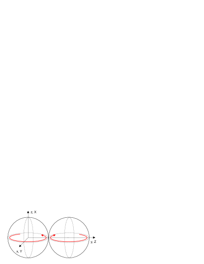
Figure 1: Configuration of a two-sphere system and possible coordinate systems. Arrowed lines show schematically two single-sphere fundamental modes

In a coordinate system with polar axis along the line of symmetry of the system ($XYZ$ system in Fig.1) the translation coefficients are diagonal in $m$ and the normal modes of the coupled system can again be classified according to the azimuthal numberMiyazaki and Jimba (2000); Deych and Roslyak (2006). However, the field distribution corresponding to the fundamental mode of the $xyz$ coordinate system cannot be characterized by a VSH with a single $m$ in the $XYZ$ system. In order to describe the same field distribution in the new coordinates one has to use transformation properties of VSHMishchenko et al. (2002) and express a single $|L,L,1\rangle$ mode of $xyz$ system as a linear combination of all $|L,m,1\rangle$ modes of the $XYZ$ system. In order to reproduce such field configuration in a single sphere we choose the incident field to be TE polarized with expansion coefficients of the form

$$\eta_{l,m}^{(i)}=\delta_{lL}\delta_{i1}R_{Lm},\hskip 5.0ptR_{Lm}=\frac{(-i)^{L}}{2^{L}}\sqrt{\displaystyle{\frac{(2L)!}{(L+m)!(L-m)!}}}$$ (3)

which is dictated by the transformation properties of VSH.

Fundamental modes in the bi-sphere

Since translational coefficients in the new coordinate system become diagonal in $m$, expansion coefficients in Eq.(1) and (2) with different values of the azimuthal number become independent and can be solved separately. In what follows we will also neglect the cross-polarization terms, described by coefficients $B_{lm}^{l^{\prime}m}$, which are usually much smaller than $A_{lm}^{l^{\prime}m}$Miyazaki and Jimba (2000). Then we need only to be concerned with coefficients $b_{lm}$ and Eq.(2). In order to understand qualitatively the effect of the coupling on the field distribution in the bi-sphere we will first solve this equation in so called single-mode approximation neglecting interaction between modes with different $l$-numbers (see details in Ref.Miyazaki and Jimba (2000); Deych and Roslyak (2006)). Expression for the scattered field in this approximation can be presented in the following form

$$\begin{split}\mathbf{E_{s}}=\frac{1}{2}\sum_{m}R_{Lm}\left[\frac{\mathbf{M}_{Lm}(\mathbf{r}-\mathbf{r}_{1})+\mathbf{M}_{Lm}(\mathbf{r}-\mathbf{r}_{2})}{\alpha_{L}^{-1}-A_{Lm}^{Lm}(\mathbf{r}_{2}-\mathbf{r}_{1})}\right.\\ \left.\frac{\mathbf{M}_{Lm}(\mathbf{r}-\mathbf{r}_{1})-\mathbf{M}_{Lm}(\mathbf{r}-\mathbf{r}_{2})}{\alpha_{L}^{-1}+A_{Lm}^{Lm}(\mathbf{r}_{2}-\mathbf{r}_{1})}\right],\end{split}$$ (4)

which gives a clear physical picture of the phenomenon under consideration. This expression describes an optical response with resonances at two sets of frequencies: one is given by the zeroes of $\alpha_{L}^{-1}-A_{Lm}^{Lm}$ and the other by the zeroes of $\alpha_{L}^{-1}+A_{Lm}^{Lm}$. The role of coupling between spheres is described by translation coefficients $A_{Lm}^{Lm}$, which shifts resonant frequency from the single sphere values by different amounts for different values of $m$. As a result terms with different azimuthal numbers resonate at different frequencies so that one ideally could expect $2(L+1)$ resonance peaks in the optical response of the system contrary to the coupled-mode theory expectation of just two resonances. The number of observable peaks is smaller because frequency shifts for higher values of $|m|$ are small and resonances from respective terms may not be distinguishable.

One can notice that the numerators of terms in Eq.(4) corresponding to different values of $m$ have a form of symmetric and antisymmetric combinations of respective single sphere modes, which is typical for the coupled mode approaches. In our consideration, however, this combination appears for every $m$-component constituting the fundamental mode separately, rather than for the entire single sphere mode.

Additional deviations from the coupled-mode approximation appear due to coupling between modes with different values of the angular number $l$, which is neglected in the single-mode approximation. This approximation can be improved by perturbation methods described in Ref.Miyazaki and Jimba (2000); Deych and Roslyak (2006), in this paper, however, we will rely on exact numerical treatment of Eq.(2).

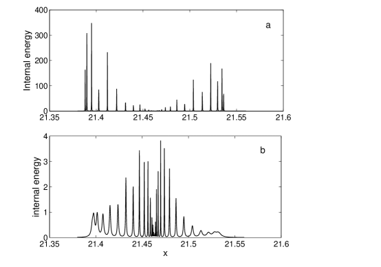
Figure 2: Frequency dependence of the internal energy of the bi-sphere in the vicinity of single sphere resonance frequency x=21.46 corresponding to a TE mode $|29,m,1\rangle$. (a) single-mode approximation; (b) numerical calculations including all modes with $l\leq 29$

For numerical analysis of Eq.(2) with incident field in the form of Eq.(3) we chose $L=29$ and spectral interval in the vicinity of resonance frequency of the mode with radial number $s=1$, $x_{29,1}=21.46$. We solve this equation using matrix inversion and including all coefficients with $l\leq L$. The limitations for the number of modes from above is made only to shorten the required time of calculation, but it does not affect the results significantly: we extended the number of included modes up to $l=48$ for several values of the dimensionless frequency $x$ and observed good convergence of the results with only small quantitative changes resulting from contribution of the modes with $l>L$. Taking into account the coefficients with $l<L$, however, is significant because some modes with smaller values of $l$ might have spectral overlap with the main mode $l=L$ and their contribution can be resonantly enhancedMiyazaki and Jimba (2000); Deych and Roslyak (2006). Using found scattering coefficients we calculate expansion coefficients of the internal field $d_{l,m}$:

$$d_{lm}^{(i)}=\frac{i}{x}\frac{1}{j_{l}(x)[nxj_{l}(nx)]^{\prime}-j_{l}(nx)[xj_{l}(x)]^{\prime}}b_{lm}^{(i)}$$ (5)

where $j_{l}(x)$ is the spherical bessel function and $[zj_{l}(z)]^{\prime}$ means differentiation with respect to $z$. Knowing coefficients $d_{lm}$ we can find total energy of the field concentrated inside spheres as a function of frequency, which is best suited to characterize optical response of our system in the spectral range of high-Q WGMsMiyazaki and Jimba (2000). Fig.2 presents the spectra of the internal energy obtained by two procedures: (a) calculations based on the single-mode approximation, Eq.(4), and (b) multi-mode numerical calculations described above. One can see that while the single-mode model reproduces the multi-resonance optical response, it deviates strongly from exact numerical calculations in positions and heights of the respective peaks. The most striking difference is significant lowering of the heights of the peaks when inter-mode coupling is taken into account, which indicates a large (three orders of magnitude) reduction of Q-factors of some of the resonances due to coupling to low-Q modes with $l\leq L$.

In order to further elucidate the role of the inter-mode coupling we consider the coefficients of the internal field $d_{lm}$ for all values of $0<l\leq 29$ and respective values of $|m|\leq l$. In order to visualize the results we present pairs $l,m$ as an one-dimensional array ordered according to the following rule $(29,-29),(29,-28),\ldots,(29,0),(29,1)$, $\ldots,(29,29),(28,-28),\ldots$ and plot coefficients $d_{lm}$ versus a number of the respective pair in this array. Fig. 3 presents the results of these calculations for $l\geq 25$ for one of the resonance frequencies, $x=21.415$. One can see that the largest values of the coefficients correspond to the main angular number $l=29$, which as a function of $m$ shows two large symmetric peaks for $m=\pm 4$. The positions of the peaks are determined by the dependence of the resonant frequency on the azimuthal number: the resonance at the chosen frequency results from the component of the internal field with $|m|=4$. In addition to main coefficients corresponding to $l=29$ the plot reveals presence of other coefficients as well. The second largest coefficient corresponds to $l=25$, which is in agreement with the fact that a frequency of the mode $|25,m,2\rangle$ is almost in resonance with our main mode, $|29,m,1\rangle$Miyazaki and Jimba (2000). While individual contributions from modes with $l<29$ appears to be small, their cumulative effect is significant as evidenced by Fig.2. The role of the inter-mode coupling can be even more important if one attempts to excite other fundamental modes such as TE mode $|39,39,1\rangle$. This mode interacts resonantly with TE modes, $|34,m,2\rangle$Miyazaki and Jimba (2000); Deych and Roslyak (2006) because of their large Q-factors and significant spectral overlap with $|39,39,1\rangle$. Deviations from single mode approximation in this case will be even more drastic.

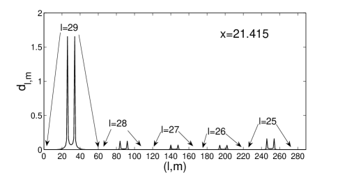
Figure 3: Internal field coefficients for all values of $l$ and $m$ for $l\geq 25$. Arrows indicate the regions corresponding to coefficients with given $l$ and varying $m$.

Conclusion

In this paper we studied effects of optical coupling on the fundamental modes excited in two spherical microresonators. We found that the optical response of this system under these excitation conditions is characterized by a rich spectrum with multiple resonances in contrast with just two peaks predicted by simplified coupled-mode type approaches. These multiple resonances arise due to the fact that strongly coupled fundamental modes of single spheres do not constitute a normal mode of a bi-sphere and must, therefore, be described by a linear combination of vector spherical harmonic with different azimuthal numbers. Optical coupling removes degeneracy between resonances with different $m$, causing, therefore, different $m$-components of the field to resonate at different frequencies and producing multi-peak spectrum. We also showed that coupling between modes with different angular numbers $l$ also significantly affects spectrum and the field distribution in the bi-sphere.

The question arises, however, how do our results agree with observations of bonding and anti-bonding orbitals with two split frequencies reported in many works? First of all, modes observed in many experiments were true normal modes of the bi-spheres, characterized by a well defined azimuthal number $m$ Rakovich et al. (2004)). These modes, however, are not coupled fundamental modes and results of this work do not apply to those experiments.

In order to observe effects presented in this paper one needs to excite a fundamental mode in a single sphere concentrated in a plane that would contain centers of both spheres, and measure optical response of the bi-sphere under the same excitation conditions. This might be possible with the use of tapered fiber excitation techniquesSpillane et al. (2003), one, however, should be aware of sensitivity of the multiple peak response to the strength of coupling and Q-factors of the modes. Increasing distance between the spheres in our numerical simulations, we observed how multiple peaks collapse to form a double peak structure. It would be a mistake, however, to associate these two peaks with the bonding and anti-bonding states of the coupled-mode theory because these peaks arise due to smearing of original multiple peaks rather than due to splitting of a single sphere resonance. The width of those peaks would represent an inhomogeneous broadening caused by inability to resolve the fine structure the spectrum rather than the radiative decay rate of respective modes.

One can see, therefore, that the picture of two coupled fundamental modes, which is used widely in modeling of optical networks can be misleading, and we hope that this work will serve as a warning that one needs to exercise caution when analyzing experimental data and developing theoretical models based on this picture.

References

- Spillane et al. (2002) S. M. Spillane, T. J. Kippenberg, and K. J. Vahala, Nature 415, 621 (2002).
- Braginsky et al. (1989) V. M. Braginsky, M. L. Gorodetsky, and V. S. Ilchenko, Phys. Lett. A 137, 393 (1989).
- Almeida et al. (2004) V. R. Almeida, C. A. Barrios, R. R. Panepucci, and M. Lipson, Nature 431, 1081 (2004).
- Ilchenko et al. (2001) V. S. Ilchenko, M. L. Gorodetsky, X. S. Yao, and L. Maleki, Opt. Lett. 26, 256 (2001).
- Bayer et al. (1998) M. Bayer, T. Gutbrod, J. P. Reithmaier, A. Forchel, T. L. Reinecke, and P. A. Knipp, Phys. Rev. Lett. 81, 2582 (1998).
- Rakovich et al. (2004) Y. P. Rakovich, J. F. Donegan, M. Gerlach, A. L. Bradley, T. M. Connolly, J. J. Boland, N. Gaponik, and A. Rogach, Phys. Rev. A 70, 051801 (2004).
- Mukaiyama et al. (1999) T. Mukaiyama, K. Takeda, H. Miyazaki, Y. Jimba, and M. Kuwata-Gonokami, Phys. Rev. Lett. 82, 4623 (1999).
- Miyazaki and Jimba (2000) H. Miyazaki and Y. Jimba, Phys. Rev. B 62, 7976 (2000).
- Spillane et al. (2003) S. M. Spillane, T. J. Kippenberg, O. J. Painter, and K. J. Valhala, Phys. Rev. Lett. 91, 043902 (2003).
- Haus et al. (1997) H. A. Haus, W. P. Huang, S. Kawakami, and N. A. Whitaker, J. Lightwave Technol. 15, 998 1005 (1997).
- Little et al. (1987) B. E. Little, S. T. Chu, H. A. Haus, J. Foresi, and J. P. Laine, J. Lightwave Technol. LT-5, 16 (1987).
- Povinelli et al. (2005) M. L. Povinelli, S. G. Johnson, M. Lonc̆ar, M. Ibanescu, E. J. Smythe, F. Capasso, and J. D. Joannopoulos, Optics Express 13 (2005).
- Naweed et al. (2005) A. Naweed, G. Farca, S. I. Shopova, and A. T. Rosenberger, Phys. Rev. A 71, 043804 (2005).
- Fuller (1991) K. A. Fuller, Applied Optics 30, 4716 (1991).
- Mishchenko et al. (2002) M. I. Mishchenko, L. D. Travis, and A. A. Lacis, Scattering, Absorption and Emission of Light by Small Particles (Cambridge University Press, Cambridge, 2002).
- Cruzan (1962) O. Cruzan, Q. Appl. Math. 20, 33 (1962).
- Stein (1961) S. Stein, Q. Appl. Math. 19, 15 (1961).
- Deych and Roslyak (2006) L. Deych and A. Roslyak, Phys. Rev. E 73, 036606 (2006).