Localization of elastic deformation in strongly anisotropic, porous, linear materials with periodic microstructures: exact solutions and dilute expansions

Abstract

Exact solutions are derived for the problem of a two-dimensional, infinitely anisotropic, linear-elastic medium containing a periodic lattice of voids. The matrix material possesses either one infinitely soft, or one infinitely hard loading direction, which induces localized (singular) field configurations. The effective elastic moduli are computed as functions of the porosity in each case. Their dilute expansions feature half-integer powers of the porosity, which can be correlated to the localized field patterns. Statistical characterizations of the fields, such as their first moments and their histograms are provided, with particular emphasis on the singularities of the latter. The behavior of the system near the void close packing fraction is also investigated. The results of this work shed light on corresponding results for strongly nonlinear porous media, which have been obtained recently by means of the “second-order” homogenization method, and where the dilute estimates also exhibit fractional powers of the porosity.

I Introduction

I.1 Context

Most of the currently available homogenization methods for strongly non-linear composites make use an underlying linear homogenization estimate, whether aimed at computing dielectric (Willis, 1986; Zeng et al., 1988; Ponte Castañeda, DeBotton, Li, 1992), or elastic-plastic transport properties (Ponte Castañeda, 1991; Ponte Castañeda, 1996; Masson et al., 2000; Ponte Castañeda, 2002; Lahellec and Suquet, 2004). The best results are obtained using an anisotropic linear estimate, the anisotropy of which is consistently determined, by the means and variances of the fields in each phase of the composite (Pellegrini, 2001; Ponte Castañeda, 2001). The anisotropy of the underlying linear medium accounts for the privileged direction imposed by the driving field in the non-linear medium.

Applying the “second-order” method (Ponte Castañeda, 2002) to a random power-law material weakened by aligned cylindrical voids, it has been found that in the so-called “dilute” limit (i.e., that of a vanishingly small volume fraction of porosity $f$), and in the limit of infinite exponent where the matrix becomes ideally plastic with a yield threshold, the leading correction to the yield stress in pure shear behaves as $f^{2/3}$. This result holds for both Hashin-Shtrikman and self-consistent estimates. The second-order method of Pellegrini (2001), suitably modified by replacing a Gaussian ansatz for the field distributions by a Heaviside ansatz (so as to cut-off high fields in a way compatible with threshold-type materials), provides in some cases similar predictions (Pellegrini and Ponte Castañeda, 2001, unpublished). This $f^{2/3}$ dilute behavior is unusual in the context of effective-medium theories for random media, where the low-order terms in dilute expansions from the literature usually consist in integer powers of $f$. With the $f^{2/3}$ correction, the derivative of the yield stress with respect to the porosity is infinite at $f=0$, due to the exponent being lower than 1. Thus, a vanishingly small volume fraction of voids induces a dramatic weakening of the porous medium. Ponte Castañeda (1996, 2002) interprets this phenomenon as an indication of localizing behavior in a regime where shear bands pass through the pores, remarking that the limit analysis of Drucker (1966) produces an upper bound for the yield threshold with a dilute correction behaving as $f^{1/2}$ in 2D. Numerical calculations and tests on perforated plates with periodically distributed holes (Francescato and Pastor, 1998) are consistent with these predictions in a plane stress situation. However, for a square network of circular holes, kinematic and static limit analyses result in the following analytical bounds on the effective yield stress $\widetilde{Y}$ (Francescato et al., 2004):

$$1-2(f/\pi)^{1/2}\leq\widetilde{Y}/Y\leq(2/\sqrt{3})\left[1-2(f/\pi)^{1/2}\right],$$ (1)

where $Y$ is the yield threshold of the matrix. Numerical limit-analysis on a hollow disk model in plane strain leads to somewhat different conclusions, with a correction behaving roughly as $f^{2/3}$ for uniform strain boundary conditions,and as $f^{1/2}$ for uniform stress boundary conditions (Pastor and Ponte Castañeda,2002). However, the calculations were not sufficiently accurate to be completely definitive. On the other hand, the exponent is quite certainly associated with localizing behavior, and its presence seems to be independent on whether the system is random, periodic, or comprises a unique void (although the actual values of the exponent may be dependent on the specific microstructure considered).

Because the second-order theory with exponent $2/3$ inherits its properties from an underlying anisotropic linear effective-medium theory, whose anisotropy is consistently determined by the field variances, a natural question concerns the “localizing” properties of the anisotropic linear theory itself, and its relation with possible non-analyticities of the effective shear moduli in the dilute limit. Bearing these considerations in mind, the present paper focuses on a new exact solution for the special, but representative, case of a two-dimensional (2D) array of voids embedded in an anisotropic linear elastic matrix, in the singular limit of infinite anisotropy. We emphasize that no exact solution of a similar type is available for general non-linear periodic media, which provides additional motivation for undertaking this study.

I.2 Organization of the paper

The constitutive laws, the prescribed loading conditions and the notations are defined in Sec. II. The word “loading” refers to the prescription of either overall conditions of homogeneous stress, or of homogeneous strain in the linear medium. Both are equivalent since they are related by the effective moduli. The matrix in the composite is compressible and possesses anisotropic properties in shear. Two special limits of infinite anisotropy which lead to exact results are then considered (Secs. III and IV). For each of these limits, simple shear, pure shear, and equibiaxial loading situations are examined, and solutions are provided in each case (for some loading and anisotropy conditions however, only the limit of an incompressible matrix is considered; but this limit is the one relevant to non-linear homogenization of plastic porous media). The effective moduli and their dilute expansions, together with the mean and variance of the strain and stress fields are computed in each case. All these quantities are relevant to non-linear homogenization theories. A useful way of condensing the information contained in the solutions is by using field distributions which can in principle directly be used to compute the effective energy (Pellegrini, 2001) or, more trivially, the moments of the fields. Local extrema or saddle points in the field maps induce singularities in the distributions such as power or logarithmic divergences, or discontinuities, of the types observed in the density of states of a crystal (Van Hove 1953; Abrikosov, Campuzano and Gofron, 1993). These singularities are examined in the context of our exact results. Cule and Torquato (1998) computed analytically the distributions of the electric field in a particular dielectric/conductor composite. They found singularities of the Van Hove type, but no extended singularities of the type put forward by Abrikosov et al. We extract below some singularities of this type, while singularities of yet a different type are encountered in Sec. IV.2.3. Obviously, in the periodic case, the field distributions are redundant with the exact solutions derived hereafter. However, for randomly disordered situations where exact solutions are not available, they remain the only way to collect useful informations on the fields. To ease their interpretation, a knowledge of their features in the periodic case is desirable, which provides a justification for the studies of Secs. III.2.4 and IV.2.3. Moreover, we find that the infinite field variances obtained for some particular loadings are correlated to field singularities directly linked to localization patterns, which have counterparts as characteristic features in the distributions. A summary of our findings and a conclusion close the paper (Sec. V).

II Problem formulation

II.1 Material constitutive law and microstructure

We consider a periodic porous medium, with a square unit cell of size $L$ made of a linear-elastic matrix (denoted by a phase index $\beta=1$), containing a single disk-shaped void of radius $a$ (phase index $\beta=2$). Cartesian reference axes $Ox$, $Oy$ are defined as in Fig. 1a, such that the void center lies at $(x,y)=(0,0)$. The unit cell is the square region $[-L/2,L/2]\times[-L/2,L/2]$. The porosity is the surface concentration of voids $f=\pi(a/L)^{2}$. The close-packing value where the voids touch is $f_{c}=\pi/4\simeq 0.78$, for $a=L/2$. Hereafter, all lengths are rescaled by $L$, so that $L\equiv 1$. The following notations are employed throughout the text: the upper-right quadrant (URQ) of the unit cell denotes the region $(x,y)\in[0,1/2]^{2}$, the lower-right quadrant (LRQ) stands for $(x,y)\in[0,1/2]\times[-1/2,0]$. Similar abbreviations ULQ and LLQ stand for the corresponding left quadrants.

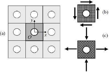
Figure 1: Left, periodic porous medium with unit cell and reference axes (a). Right, unit cell with (b) 0-type fibers; and (c) 45-type fibers. The black arrows depict eigenmodes of strain: simple shear (SS) in (b), and pure shear (PS) in (c).

Small deformations and plane strain conditions are assumed, so that the strain $\varepsilon$ derives from the two-dimensional (in-plane) displacement field $\mathbf{u}$, and $\varepsilon_{ij}=0$ if $i$ or $j=z$. In-plane stress equilibrium requires $\partial_{i}\sigma_{ij}=0$, $i,j=1,2$ and we take the constitutive relation such that $\sigma_{xz}=\sigma_{yz}=0$, so that the problem is two-dimensional. The linear constitutive relation in the medium is $\mbox{\boldmath$\sigma$}(\mathbf{x})=\mathbb{L}(\mathbf{x}):\mbox{\boldmath$\varepsilon$}(\mathbf{x})$. In the voids, $\mathbb{L}(\mathbf{x})\equiv 0$. In the anisotropic matrix phase, $\mathbb{L}(\mathbf{x})$ has components (Latin indices henceforth vary over 1 and 2):

$$L_{ij,kl}^{(1)}=2\kappa\,J_{ij,kl}+2\lambda\,E^{\rm SS}_{ij,kl}+2\mu\,E^{\rm PS}_{ij,kl},$$ (2)

where $\kappa$ is the bulk compressibility modulus, where $\lambda$, $\mu$ are in-plane anisotropic shear moduli, and where the operators $\mathbb{J}$, $\mathbb{E}^{\rm SS}$, $\mathbb{E}^{\rm PS}$ are mutually orthogonal projectors of components (no summation over repeated indices here):

$$J_{ij,kl}=\frac{1}{2}\delta_{ij}\,\delta_{kl},\quad E^{\rm SS}_{ij,kl}=\frac{1}{2}(1-\delta_{ij})(1-\delta_{kl}),\quad E^{\rm PS}_{ij,kl}=\delta_{ij}\,\delta_{kl}(\delta_{ik}-1/2).$$ (3)

A symmetric two-dimensional tensor $\mathsf{a}$ is expanded as $\mathsf{a}=a_{\text{m}}\,\mathsf{I}+a_{\text{SS}}\,\mathsf{e}_{SS}+a_{\rm PS}\,\mathsf{e}_{\rm PS}$ where $\mathsf{I}$ is the $2\times 2$ identity matrix and where:

$$\mathsf{e}_{\rm SS}=\left(\begin{array}[]{cc}0&1\\ 1&0\end{array}\right),\qquad\mathsf{e}_{\rm PS}=\left(\begin{array}[]{cc}1&0\\ 0&-1\end{array}\right),$$ (4)

the eigenvector sets of which are related by a 45-degree rotation. Corresponding strain modes are represented by arrows in Fig. 1b and 1c. The equibiaxial component of $\mathsf{a}$ is $a_{m}\equiv(a_{xx}+a_{yy})/2$. We call the second and third components the simple shear (SS) and pure shear (PS) components, with $a_{\text{SS}}\equiv a_{xy}$ and $a_{\text{\rm PS}}\equiv(a_{xx}-a_{yy})/2$. Then $\mathbb{J}:\mathsf{a}=a_{m}\mathsf{I}$, $\mathbb{E}^{\rm SS}:\mathsf{a}=a_{\text{SS}}\,\mathsf{e}_{SS}$ and $\mathbb{E}^{\rm PS}:\mathsf{a}=a_{\text{PS}}\,\mathsf{e}_{\rm PS}$. Accordingly, the constitutive relations decompose into:

$$\sigma_{\rm SS}=2\lambda\,\varepsilon_{\rm SS},\qquad\sigma_{\rm PS}=2\mu\varepsilon_{\rm PS},\qquad\sigma_{\text{m}}=2\kappa\,\varepsilon_{\text{m}}.$$ (5)

Elastic tensor (2) is of a special type of orthotropy in the plane with $L_{1111}=L_{2222}\not=L_{1122}\not=L_{1212}$. When $\lambda>\mu$, this type of anisotropic response could correspond to a fiber-reinforced material with fibers aligned with the cell axes (see Fig. 1b). On the other hand, when $\mu>\lambda$, it would correspond to a material with reinforcing fibers aligned with the $\pm 45^{\rm o}$ direction (see Fig. 1c). We introduce a shear anisotropy ratio, $\alpha$, and normalized shear elastic moduli, $m$ and $\ell$:

$$\alpha=\lambda/\mu,\qquad m=\mu/\kappa,\qquad\ell=\lambda/\kappa.$$ (6)

The principal directions of the matrix being “aligned” with dense lines of voids, a reinforcement of anisotropy-induced effects is expected. Besides, the loading modes considered below are aligned with the eigenstrains. These choices, motivated by future applications of this work to non-linear homogenization, focus on situations most relevant to plastic localization in porous media. Indeed, in the nonlinear theory, the loading determines the anisotropy of the background linear medium and always coincides with one of its eigendirections. Moreover, shear bands in random porous media quite generally link neighboring voids together.

II.2 Overall behavior

In this work, we are concerned with the problem of determining the overall behavior of the periodic, porous material described in the previous subsection. This overall behavior is defined as the relation between the average stress $\langle\mbox{\boldmath$\sigma$}\rangle$ and the average strain $\langle\mbox{\boldmath$\varepsilon$}\rangle$. Under the assumption of separation of length scales, the overall behavior of the porous material may be determined from the effective strain potential (see Torquato, 2002)

$$W=(1-f)\mathop{\min}\limits_{\mbox{\boldmath$\varepsilon$}\in\mathcal{K}}\left\langle w^{(1)}(\mbox{\boldmath$\varepsilon$})\right\rangle_{(1)},$$ (7)

where $\left\langle\cdot\right\rangle_{(1)}$ denotes an average over the matrix phase, $w^{(1)}(\mbox{\boldmath$\varepsilon$})=(1/2)\mbox{\boldmath$\varepsilon$}:\mathbb{L}^{(1)}:\mbox{\boldmath$\varepsilon$}$ is the strain potential in the matrix and $\mathcal{K}=\{\mbox{\boldmath$\varepsilon$}\,|\mbox{\boldmath$\varepsilon$}=(1/2)\left[\nabla\mathbf{u}+(\nabla\mathbf{u})^{T}\right],$ $\mathbf{u}=\langle\mbox{\boldmath$\varepsilon$}\rangle\mathbf{x}+\mathbf{u}^{*},$ $\mathbf{u}^{*}\ {\rm periodic}\}$ is the set of kinematically admissible strain fields. The overall constitutive relation is then given by

$$\langle\mbox{\boldmath$\sigma$}\rangle=\frac{\partial W}{\partial\langle\mbox{\boldmath$\varepsilon$}\rangle}.$$ (8)

Because of linearity, we define the overall elasticity tensor $\widetilde{\mathbb{L}}$ of the porous material via the relation $\langle\mbox{\boldmath$\sigma$}\rangle=\widetilde{\mathbb{L}}:\langle\mbox{\boldmath$\varepsilon$}\rangle$. This tensor can be shown to take on the same form as (2) with components ${\widetilde{L}}_{ij,kl}$ defined by effective moduli $\widetilde{\lambda}$, $\widetilde{\mu}$ and $\widetilde{\kappa}$.

In the analyses below, it will sometimes be more convenient to work with the effective stress potential $U$, such that the overall constitutive relation may be equivalently written

$$\langle\mbox{\boldmath$\varepsilon$}\rangle=\frac{\partial U}{\partial\langle\mbox{\boldmath$\sigma$}\rangle},\quad U=(1-f)\mathop{\min}\limits_{\mbox{\boldmath$\sigma$}\in\mathcal{S}}\left\langle u^{(1)}(\mbox{\boldmath$\sigma$})\right\rangle_{(1)},$$ (9)

where $u^{(1)}(\mbox{\boldmath$\sigma$})=(1/2)\mbox{\boldmath$\sigma$}:\left(\mathbb{L}^{(1)}\right)^{-1}:\mbox{\boldmath$\sigma$}$ is the stress potential in the matrix and $\mathcal{S}$ denotes the set of periodic stresses that are divergence-free in the unit cell, with prescribed average $\langle\mbox{\boldmath$\sigma$}\rangle$, and traction-free on the boundaries of the pores. It should be noted that the case of an isotropic matrix ($\alpha=1$) has been addressed by McPhedran and Movchan (1994) in the more general framework of arbitrary contrast between the matrix and the square array of isotropic inclusions.

II.3 Limits of infinite anisotropy and loading modes

Hereafter only the strong anisotropy limits $\alpha=0$ and $\alpha=+\infty$, amenable to an exact solution, are considered. Therefore: (i) When $\alpha=0$ (i.e., $\lambda=0$ or $\mu=\infty$) the medium is soft for SS loading, and resists PS loading; (ii) When $\alpha=\infty$ (i.e., $\lambda=\infty$ or $\mu=0$) the medium is soft for PS loading, and resists SS loading. Equibiaxial, SS and PS loading modes will be considered separately hereafter, so that only one of the three averaged components of the strain or stress is non-zero at a time. It is denoted by $\overline{\varepsilon}$ (resp. $\overline{\sigma}$). Depending on the loading mode considered, strain and stress components and displacements enjoy various symmetry properties summarized in Appendix A.

For clarity, we detail the correspondence between the loading modes and the anisotropy properties of the material. Consider e.g. the limiting case $\alpha=\lambda/\mu\to 0$, attained by two different types of materials: (i) $\lambda\to 0$ and $\mu>0$ (Material 1); (ii) $\mu\to\infty$ and $\lambda<\infty$ (Material 2). We seek solutions with strain and stress finite almost everywhere (a.e.), i.e., except on points or on lines in the plane. In particular, $\sigma_{\text{PS}}=2\mu\,\varepsilon_{\text{PS}}$ is finite a.e., so that $\varepsilon_{\text{PS}}\equiv 0$ a.e. in Material 2. Likewise $\varepsilon_{\text{SS}}=\sigma_{\text{SS}}/(2\lambda)$ is finite a.e., so that $\sigma_{\text{SS}}\equiv 0$ a.e. in Material 1. Hence Material 1 is infinitely soft in the SS direction and can be finitely loaded in the PS direction, whereas Material 2 is infinitely rigid in the PS direction and can be finitely loaded only in the SS direction. Similar considerations apply for $\alpha=\infty$, leading to the following correspondence:

$\alpha=0$:     PS loading $\leftrightarrow$ $\lambda=0$,    SS loading $\leftrightarrow$ $\mu=\infty$,

$\alpha=\infty$:  SS loading $\leftrightarrow$ $\mu=0$,   PS loading $\leftrightarrow$ $\lambda=\infty$.

In equibiaxial loading, both types of materials should be considered for each of the limits $\alpha=0$ or $\alpha=\infty$.

As is well-known, the elasticity tensor (2) is positive definite when $\lambda$, $\mu$ and $\kappa$ are all strictly positive, and we have existence and uniqueness of solutions. As mentioned above, however, the interest in this work is for the limiting cases where one of the eigenvalues of the elasticity tensor (2) (or, of its inverse, the compliance tensor) tend to zero. For these cases, care must be exercised when interpreting the solutions. As will be seen below, the relevant potential energy, or complementary energy functionals can still be shown to be strictly convex in the subspace of allowable strains, or stresses, and the standard theorems (see, for example, Proposition 1.2 of Ekeland and Temam, 1974) would still ensure existence and uniqueness of the solutions. However, appropriate components of the strain (or stress) field can develop discontinuities in these limiting cases. In this connection, it is also relevant to note that the governing equations lose ellipticity, leading to hyperbolic behavior (see below). This phenomenon is well-known in two-dimensional problems for ideally plastic materials (Kachanov, 1974), and has been exploited in a recent study of shape-memory polycrystals (Chenchiah and Bhattacharya, 2005). As was shown in this later reference, the hyperbolicity of the equations can be very helpful in interpreting the solutions obtained, and such connections will be made for the specific cases to be considered below. In any case, it should be kept in mind that the solutions of interest here are limiting cases of standard elasticity problems (with positive-definite elasticity tensors) for which solutions have been obtained by numerical methods (Willot et al., 2007).

II.4 Hyperbolicity conditions and characteristics

Making use of the constitutive relations (5), the stress equilibrium conditions may be written in terms of the displacement field as a closed system of two second-order partial differential equations (PDEs):

$$\left(\begin{array}[]{cc}\mu+\kappa&0\\ 0&\lambda\end{array}\right)\partial_{x}^{2}\mathbf{u}+\left(\begin{array}[]{cc}\lambda&0\\ 0&\mu+\kappa\end{array}\right)\partial_{y}^{2}\mathbf{u}+(\lambda+\kappa-\mu)\left(\begin{array}[]{cc}0&1\\ 1&0\end{array}\right)\partial_{x}\partial_{y}\mathbf{u}=0.$$ (10)

Following Otto et al. (2003), this system is decoupled as:

$$Du_{i}=0,\quad D\varepsilon_{ij}=0,\quad D\sigma_{ij}=0,\qquad i=x,y,\quad j=x,y,$$ (11)

where the PDEs for the strain and stress fields follow immediately, and where $D$ is the fourth-order differential operator:

$$D=\partial_{x}^{4}+\partial_{y}^{4}+2r\partial_{x}^{2}\partial_{y}^{2},\quad r=\frac{\lambda(\mu-\kappa)+2\kappa\mu}{\lambda(\mu+\kappa)}.$$ (12)

This PDE has the symbolic form $\phi(x,y)=x^{4}+y^{4}+2rx^{2}y^{2}$, with characteristic lines (e.g., Zachmanoglou and Thoe, 1986) defined by the equation $\phi(\textnormal{d}x,\textnormal{d}y)=0$, such that:

$$\frac{\textnormal{d}x}{\textnormal{d}y}=\pm\sqrt{-r\pm(r^{2}-1)^{1/2}}.$$ (13)

Taking $\lambda$, $\mu$, $\kappa\geq 0$, $r$ lies on the segment line $r\in[-1,\infty)$. At any interior point $-1<r<\infty$, the quantity $\textnormal{d}x/\textnormal{d}y$ is strictly complex; there are no characteristic lines in the real plane and the problem is elliptic. This corresponds to either (i) $0<\lambda,\mu<\infty$; (ii) $0<\mu<\infty$, $\lambda=\infty$, $\kappa<\infty$; (iii) $0<\lambda<\infty$, $\mu=\infty$, $\kappa<\infty$. At the end points $r=-1$ and $r=\infty$, the form $\phi(\textnormal{d}x,\textnormal{d}y)$ has two distinct real roots for $\textnormal{d}x/\textnormal{d}y$, each of them of multiplicity two. Thus the problem becomes hyperbolic with straight characteristics $x/y=cst$:

Case 1: $$r=\infty\quad\Leftrightarrow\quad\lambda=0\textnormal{ or }\mu=\kappa=\infty\quad\Leftrightarrow\quad x,y=cst,$$ (14)

Case 2: $$r=-1\quad\Leftrightarrow\quad\mu=0\textnormal{ or }\lambda=\kappa=\infty\quad\Leftrightarrow\quad x=\pm y+cst.$$ (15)

In this study, only hyperbolic problems are considered, i.e. the medium will be taken incompressible ($\kappa=\infty$) when $\lambda$ or $\mu=\infty$. All characteristics encountered are straight lines aligned with either one of the Cartesian axes ($\alpha=0$) or with one of the two diagonals of the unit cell ($\alpha=\infty$). As will be seen, the solutions found for the stress, strain or displacement fields actually verify simpler, first or second-order PDEs which can be used instead of (11).

II.5 Averages, standard deviations and field distributions

For any stress or strain component $a(\mathbf{x})$ produced by a loading $\overline{a}$, normalized phase averages and standard deviations in phase $\beta$ are defined as:

$$M^{(\beta)}(a)\equiv\langle a\rangle_{(\beta)}/\overline{a},\qquad S^{(\beta)}(a)\equiv\sqrt{\langle a^{2}\rangle_{(\beta)}-\langle a\rangle_{(\beta)}^{2}}/\overline{a}.$$ (16)

The distribution (i.e. the histogram) of $a$ in the matrix $M$, $P_{a}(t)$, is obtained by counting occurrences with the Dirac distribution $\delta$. All individual averages in the matrix result from the definition $\langle g(a)\rangle_{(1)}=\int{\rm d}t\,g(t)P_{a}(t)$, where:

$$P_{a}(t)\equiv(1-f)^{-1}\int_{M}\!\,\text{d}^{2}\!x\,\delta(a(\mathbf{x})-t).$$ (17)

III Material with anisotropy ratio $\alpha=0$

III.1 Loading in pure shear

In this section, $\alpha=0$ with $\lambda=0$. A PS stress loading $\overline{\sigma}=\langle\sigma_{\rm PS}\rangle$ is applied.

III.1.1 Stress fields

Using (5), $\lambda=0$ implies $\sigma_{\text{SS}}=\sigma_{xy}\equiv 0$. Then, from stress equilibrium,

$$\sigma_{xx}(x,y)=g(y),\quad\sigma_{yy}(x,y)=-g(x),$$ (18)

where $g$ is an unknown 1-periodic function (using symmetry 91). Hence:

$$\sigma_{\text{PS,m}}=[g(y)\pm g(x)]/2,$$ (19)

where the plus (resp. minus) sign applies to $\sigma_{\text{PS}}$ (resp. $\sigma_{\text{m}}$). This sign convention for PS loading, repeatedly employed hereafter, only holds for Sec. III.1. The opposite convention will apply in Secs. III.2 and III.3.

We note that each stress component $\sigma_{ii}$ (no summation) obeys a simple first-order PDE, where $x=cst$ and $y=cst$ are characteristic lines, in agreement with (14). The stress vanishes in the void so that $g(x)\equiv 0$ for $x\in[-a,a]$. The structure of the solution is most easily grasped referring to Fig. 2(a). It is organized in three types of zones: (A), (B), and (D), separated by “frontiers” marked by solid lines. The PS stress reduces to $\sigma_{\text{PS}}=g(x)/2$ or $g(y)/2$ in zone (B), to $\sigma_{\text{PS}}=0$ in zone (D), and to $\sigma_{\text{PS}}=[g(x)+g(y)]/2$ in zone (A). It thus vanishes in the square of length $2a$ consisting in the union of (D) and of the void (V). This is more easily understood in terms of characteristics. Since the transverse stress component $\sigma_{xy}$ is zero, the void boundary conditions for the stress reduces to $\sigma_{xx}=\sigma_{yy}=0$ at any point of the void-matrix interface. Hence, each of these components is zero along one of the two families of characteristics (vertical or horizontal) passing through a void. At the intersection of characteristic lines passing through a void (i.e. region D), all stress components must be zero. Thus, as far as stress is concerned, the voids behave as square voids. In particular, the effective modulus (34a) must be a natural function of $a$ rather than of $f$ (i.e. must not contain $\pi$ when expressed in terms of $a$).

(a)      (b) Figure 2: Structure of field patterns in the unit cell, in situations of infinite anisotropy. Figure (a): pattern for $\alpha=0$. Figure (b): $\alpha=\infty$ (cf. Sec. IV).

The unknown function $g$ is obtained by minimizing the complementary elastic energy functional (9), which is a strictly convex problem in the subspace of periodic stress fields with vanishing $SS$ component (i.e., $\sigma_{\text{SS}}=0$):

$$(1-f)\langle u^{(1)}(\mbox{\boldmath$\sigma$})\rangle_{(1)}=\int_{-\frac{1}{2}\leq x,y\leq\frac{1}{2}}\left[\frac{1}{2\mu}\sigma_{\text{PS}}^{2}(x,y)+\frac{1}{2\kappa}\sigma_{\text{m}}^{2}(x,y)\right]\,{\rm d}x\,{\rm d}y,$$

$$\qquad\qquad\qquad=\frac{1}{2}\left(\frac{1}{\mu}+\frac{1}{\kappa}\right)\int_{a}^{1/2}g^{2}(x)\,{\rm d}x+\left(\frac{1}{\mu}-\frac{1}{\kappa}\right)\left[\int_{a}^{1/2}g(x)\,{\rm d}x\right]^{2}.$$

Functionally extremizing this integral with respect to $g$ under the constraint

$$\langle\sigma_{\text{PS}}\rangle=\overline{\sigma}=2\int_{a}^{1/2}\!\!\!\!\!\!g(x)\,{\rm d}x$$ (20)

provides $g(x)\equiv\overline{\sigma}/(1-2a)$ for $x\in[-1/2,-a]\cup[a,1/2]$. Denoting by $\theta_{[x_{1},x_{2}]}(z)$ the characteristic function of the interval $[x_{1},x_{2}]$, we introduce $\chi(z)\equiv 1-\theta_{[-a,a]}(z)$, the characteristic function of the domain $[-1/2,-a]\cup[a,1/2]$. Then, $\sigma_{\text{PS}}$ and $\sigma_{\text{m}}$ are completely determined by:

$$\sigma_{\text{PS,\,m}}(x,y)=\overline{\sigma}\frac{\chi(y)\pm\chi(x)}{2(1-2a)}.$$ (21)

Referring to Fig. 2(a), $\sigma_{PS}$ meets its highest (constant) value in zones (A), is of half this value in zones (B), and zero elsewhere. The discontinuous stress pattern obtained here as a solution for infinite anisotropy is of the type used by Drucker (1966) in his limit analysis of the ideally plastic porous medium.

III.1.2 Strain field

From (6) and (21), the strain components $\varepsilon_{\text{PS}}$ and $\varepsilon_{\text{m}}$ in the matrix read:

$$\varepsilon_{\text{PS}}(x,y)=\overline{\sigma}\frac{\chi(y)+\chi(x)}{4\mu(1-2a)},\qquad\varepsilon_{\text{m}}(x,y)=\overline{\sigma}\,m\,\frac{\chi(y)-\chi(x)}{4\mu(1-2a)}.$$ (22)

The relationship between $\overline{\sigma}$ and $\overline{\varepsilon}=\langle\varepsilon_{\rm PS}\rangle$ is now obtained. To compute $\overline{\varepsilon}$, we use $\mathbf{u}^{*}$. Expressions (22) equivalently read [cf. equation (91e)]:

$$\varepsilon_{xx}(x,y)=-\varepsilon_{yy}(y,x)=\frac{1}{4\mu}\frac{\overline{\sigma}}{1-2a}[\left(1-m\right)\chi(x)+\left(1+m\right)\chi(y)].$$ (23)

In PS loading, the admissibility (i.e., compatibility) conditions in (7) imply that $\partial_{x}u^{*}_{x}=\varepsilon_{xx}-\overline{\varepsilon}$ and $\partial_{y}u^{*}_{y}=\varepsilon_{yy}+\overline{\varepsilon}$. The displacement component $u^{*}_{x}$ (resp. $u^{*}_{y}$) is odd and 1-periodic wrt. $x$ (resp. $y$, see Eqs. 91). This requires $\mathbf{u}^{*}$ to be tangent to the boundary of the unit cell: $u^{*}_{x}(\pm 1/2,y)\equiv u^{*}_{y}(x,\pm 1/2)\equiv 0$. Hence, the previous Eqs. are integrated as:

$$u_{x}^{*}(x,y)=\int^{x}_{-1/2}{\rm d}x^{\prime}\,\left[\varepsilon_{xx}(x^{\prime},y)-\overline{\varepsilon}\right],\quad u_{y}^{*}(x,y)=\int^{y}_{-1/2}{\rm d}y^{\prime}\,\left[\varepsilon_{yy}(x,y^{\prime})+\overline{\varepsilon}\right].$$ (24)

Furthermore, the periodicity condition $u^{*}_{x}(1/2,\cdot)\equiv 0$ yields:

$$\int^{1/2}_{-1/2}{\rm d}x\,\left[\varepsilon_{xx}(x,y)-\overline{\varepsilon}\right]=0.$$ (25)

Choosing, e.g., $y=1/2$ (in the matrix) and inserting (23) in (25) provides the desired relation between $\overline{\sigma}$ and $\overline{\varepsilon}$:

$$\overline{\sigma}=\frac{2\mu(1-2a)}{1+(m-1)a}\overline{\varepsilon}$$ (26)

Since $m>0$ and $0\leq a\leq 1/2$, the denominator of (26) is always $>0$.

The still unknown $\varepsilon_{xy}\equiv\varepsilon_{\text{SS}}$ is computed from the admissibility (i.e., compatibility) conditions in (7), and from the expressions of $u^{*}_{x}$ and $u^{*}_{y}$ in (24). We obtain for $(x,y)$ in the matrix:

$$\varepsilon_{xy}(x,y)=\frac{1}{2}\left[\int_{-1/2}^{x}{\rm d}x^{\prime}\frac{\partial}{\partial y}\varepsilon_{xx}(x^{\prime},y)+\int_{-1/2}^{y}{\rm d}y^{\prime}\frac{\partial}{\partial x}\varepsilon_{yy}(x,y^{\prime})\right].$$ (27)

Inserting the solutions (23), the integration is first carried out in the LLQ for integration paths in the matrix. The result is extended to the whole unit cell appealing to identities (91f,g). For instance, in the URQ:

$$\varepsilon_{\text{SS}}(x,y)=\frac{\overline{\varepsilon}}{4}\frac{1+m}{1+(m-1)a}\left[\left(x-\frac{1}{2}\right)\delta(y-a)-\left(y-\frac{1}{2}\right)\delta(x-a)\right],$$ (28)

where the Dirac distributions stem from the discontinuities in the displacements (24) due to the $\chi$ functions in (23). Hence, in PS loading, $\varepsilon_{\text{SS}}$ is localized on the four “frontier” lines in the unit cell. Points $(x,y)=(\pm a,0)$ and $(0,\pm a)$ are singular hot spots. At each tangency point of a “frontier” line with the void boundary, there occurs a jump of $\varepsilon_{\text{SS}}$ along the line. E.g., in the vicinity of $(a,0)$, (28) and the symmetry $\varepsilon_{xy}(x,-y)=-\varepsilon_{xy}(x,y)$ provide:

$$\varepsilon_{\text{SS}}(x,y)\simeq\frac{\overline{\varepsilon}}{8}\frac{1+m}{1+(m-1)a}\delta(x-a)\,\mathop{\text{sign}}y.$$ (29)

III.1.3 Displacement field and “hot spots”.

From (24) and identity $u^{*}_{x}(x,y)=-u^{*}_{x}(-x,-y)$, the displacement $\mathbf{u}^{*}$ corresponding to the above strains reads in the URQ ($\theta$ is the Heaviside function):

$$u_{x}(x,y) = \frac{\overline{\varepsilon}}{1+(m-1)a}\left\{\left(\frac{1}{2}-x\right)\left[(m-1)a+\frac{1}{2}(m+1)\theta(a-y)\right]\right.$$ (30)

$${}\left.-\frac{1}{2}(m-1)(a-x)\theta(a-x)\right\}.$$

Moreover, $u^{*}_{y}(x,y)=-u^{*}_{x}(y,x)$. Again referring to Fig. 2(a), $\mathbf{u}^{*}$ is a linear function of $x$, $y$ in (A), (B) and (D). Along the “frontiers” between (A) and (B) or between (B) and (D), its component normal to the “frontier” is continuous, whereas its tangential component is discontinuous. For instance, on the “frontier” $y=a$ for $a<x<1/2$, $u_{x}^{*}$ undergoes a jump $[[u_{x}^{*}]]_{y}\equiv u_{x}^{*}(x,a^{+})-u_{x}^{*}(x,a^{-})$ given by:

$$[[u_{x}^{*}]]_{y}(x,a)=-u_{1}(1/2-x),\qquad u_{1}\equiv\frac{\overline{\varepsilon}(1+m)}{2[1+(m-1)a]}.$$ (31)

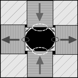
Figure 3: Structure of the deformed matrix and of $\mathbf{u^{*}}$ (arrows) for an anisotropy ratio $\alpha=0$, in the particular case of equal bulk and shear moduli $\kappa=\mu$. Loading is PS. Voids are in black. White (resp. grey) elliptic rings tag zones of extreme matter separation (resp. crushing).

As expected, the displacement field can develop discontinuities along characteristic lines. This feature is reminiscent of rigid, ideally-plastic bodies in isotropic two-dimensional materials where discontinuities may only occur tangentially to slip lines (Kachanov, 1974, prop. 39.4). The structure of the full deformed configuration is schematized in Fig. 3: overall deformation occurs by block sliding. Fig. 3 is drawn in the particular case of equal bulk and shear moduli, $\kappa=\mu$ ($m=1$). Then, $\mathbf{u^{*}}$ vanishes strictly in zone (A) — but is finite there if $\kappa\not=\mu$ — and is aligned with the axes in (B).

The expression of $\mathbf{u}$ in (D) clarifies the nature of the hot spots:

$$\mathbf{u}(x,y)=u_{1}(\mathop{\text{sign}}x,-\mathop{\text{sign}}y),\qquad-a<x,y<a,$$ (32)

We stress that this incomplete expression, valid for $-a<x,y<a$ only, does not allow one to recover the singularity (29) of $\varepsilon_{xy}$ by taking a derivative. Since $\mathbf{u}$ is constant, save for orientation changes, in the four quadrants of zone (D), the hot spots are either points of extreme matter separation (at $(x,y)=(0,\pm a)$ for $\overline{\varepsilon}>0$; white elliptic markings in Fig. 3) or of matter crushing (at $(x,y)=(0,\pm a)$; dark markings).

Fig. 3 also makes conspicuous four voided squares (in black) generated by the block-sliding pattern, at the intersections $(x,y)=(\pm a,\pm a)$ of the “frontier” lines (the phenomenon is most remarkable for $m=1$). The immediate vicinity of each of these points is divided into four regions where the displacement vector locally takes on distinct values. For instance, around $(x,y)=(a,a)$, we have $\mathbf{u^{*}}(a^{+},a^{+})=(u_{0},-u_{0})$, $\mathbf{u^{*}}(a^{+},a^{-})=(u_{0}+\Delta u,-u_{0})$, $\mathbf{u^{*}}(a^{-},a^{+})=(u_{0},-u_{0}-\Delta u)$, $\mathbf{u^{*}}(a^{-},a^{-})=(u_{0}+\Delta u,-u_{0}-\Delta u)$, where

$$u_{0}=2u_{1}[(1-m)/(1+m)]a(a-1/2),\qquad\Delta u=u_{1}(1/2-a).$$ (33)

The quantity $\Delta u$ represents the size of the voided square, to first order in $\overline{\varepsilon}$. Remark that in terms of $\overline{\sigma}$, it reads $\Delta u=\overline{\sigma}(1+m)/(8\mu)$, a void-independent expression (the dimensioning factor is the cell size $L=1$).

III.1.4 Distributions, moments and effective shear modulus $\widetilde{\mu}(f)$

In the PS case, the distributions $P_{\varepsilon_{z}}(t)$ or $P_{\sigma_{z}}(t)$ consist uniquely of a sum of Dirac-type components, plus unusual singular components at $\varepsilon_{z}\to\pm\infty$, due to the Dirac singularities in the fields. The latter cannot be accounted for by probability densities unless inconvenient limiting processes are employed. This may constitute a limitation of the use of distributions in a localizing regime. However, the first and second moments are readily computed. The effective shear modulus $\widetilde{\mu}$ is read from (26). With $a\equiv\sqrt{f/\pi}<1/2$, we have:

$$\frac{\widetilde{\mu}}{\mu}=\frac{1-2a}{1+(m-1)a}=1-(1+m)(f/\pi)^{1/2}+O(f),$$ (34a)

$$M^{(1)}(\varepsilon_{\text{PS}})=\frac{1-2a}{(1-f)[1+(m-1)a]},\quad M^{(2)}(\varepsilon_{\text{PS}})=\frac{(m+1)a}{f[1+(m-1)a]},$$ (34b)

$$S^{(1)}(\varepsilon_{\text{PS}})=\frac{\sqrt{(1-2a)[(1+f)a-f]}}{(1-f)[1+(m-1)a]},\quad S^{(1)}(\sigma_{\text{PS}})=\frac{\sqrt{(1+f)a-f}}{(1-f)\sqrt{1-2a}},$$ (34c)

$$S^{(1)}(\varepsilon_{\text{m}})=\frac{m\sqrt{a(1-2a)}}{[1+(m-1)a]\sqrt{1-f}},\quad S^{(1)}(\sigma_{\text{m}})=\sqrt{\frac{a}{(1-f)(1-2a)}},$$ (34d)

$$S^{(1)}(\varepsilon_{\text{SS}})=\infty,\quad S^{(1)}(\sigma_{\text{SS}})=0.$$ (34e)

The mean strain in the pore stems from $M^{(2)}(\varepsilon_{\text{PS}})=[1-(1-f)M^{(1)}(\varepsilon_{\text{PS}})]/f$. Moreover, $S^{(1)}(\sigma_{\text{PS}})=(\mu/\widetilde{\mu})S^{(1)}(\varepsilon_{\text{PS}})$. The Dirac singularities are responsible for the transverse variance $S^{(1)}(\varepsilon_{\text{SS}})$ being infinite. Also, remark that $M^{(2)}(\varepsilon_{\text{PS}})$ blows up as $f^{-1/2}$ when $f\to 0$. The curve $\widetilde{\mu}(f)/\mu$ is displayed in Fig. 4 in the incompressible case $m=0$. The power singularity at $f=0$ with infinite negative slope, due to the $f^{1/2}$ term in the dilute expansion of (34a), indicates that an infinitesimal void dramatically weakens the medium. This is reminiscent of the situation encountered in plasticity (see Introduction). In the linear material considered here, it is a direct consequence of hyperbolicity. Each of the two components $\sigma_{xx}$ and $\sigma_{yy}$ have constant values along one of the two families of characteristics. Due to the boundary conditions at the void-matrix interface, the parallel component $\sigma_{\textnormal{PS}}$ is smaller by half in region (B) than it is in (A). Hence, each void lowers the stress field over large regions in the material, which are projections of the voids along the characteristic directions and involve infinitely long distances. The normalized standard deviations $S^{(1)}(\varepsilon_{\text{PS}})$, $S^{(1)}(\varepsilon_{\text{m}})$, $S^{(1)}(\sigma_{\text{PS}})$ and $S^{(1)}(\sigma_{\text{m}})$ all behave as $(f/\pi)^{1/4}$ as $f\to 0$, which indicates that they grow more rapidly with $f$ than in a linear isotropic medium. The effective modulus $\widetilde{\mu}(f)$ vanishes linearly with $(f_{c}-f)$ for $f$ near $f_{c}=\pi/4$, the void close packing fraction (see the comment in Sec. III.2.2), along with the moments of the strain components in the matrix in the loading direction ($M^{(1)}(\varepsilon_{\text{PS}})$ $=$ $S^{(1)}(\varepsilon_{\text{PS}})$ $=0$).

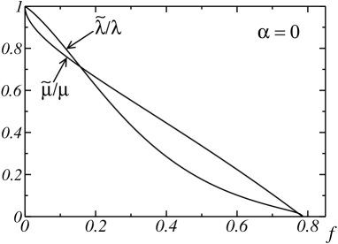
Figure 4: Normalized shear effective moduli $\widetilde{\mu}/\mu$ and $\widetilde{\lambda}/\lambda$ vs. void concentration $f$, for an incompressible matrix with anisotropy ratio $\alpha=\lambda/\mu=0$. Both moduli vanish at the close packing threshold $f=f_{c}=\pi/4\simeq 0.78$.

III.2 Loading in simple shear (incompressible case only)

According to Sec. II.3, SS loading goes along with $\alpha=0$ and $\mu=\infty$. Matrix incompressibility renders the problem hyperbolic and is assumed for simplicity ($\kappa=\infty$, $m=0$).

III.2.1 Displacement, strain and stress fields

Taking $\mu=\infty$ under finite stress implies $\varepsilon_{xx}-\varepsilon_{yy}=0$. Incompressibility then requires $\varepsilon_{xx}=\varepsilon_{yy}=0$. The only non-zero component is $\varepsilon_{xy}$, and a variational calculation is simpler to carry out wrt. the strain rather than to the stress. Condition $\varepsilon_{xx}=\varepsilon_{yy}=0$ implies $u^{*}_{x}(x,y)=u^{*}_{x}(y)$ and $u^{*}_{y}(x,y)=u^{*}_{y}(x)$. By symmetry, see 92c, $u^{*}_{x}(z)=u^{*}_{y}(z)\equiv G(z)-\overline{\varepsilon}\,z$, where $G$ is unknown. Introducing the derivative $g\equiv G^{\prime}$, one obtains:

$$\varepsilon_{xy}(x,y)=[g(x)+g(y)]/2.$$ (35)

The energy of the unit cell (7) is expressed as an integral over the matrix phase $M$ (represented by the unit square minus the void):

$$(1-f)\langle w^{(1)}\rangle_{(1)}=2\lambda\int_{M}{\rm d}^{2}\!x\,\mathsf{\varepsilon}_{xy}^{2}=\frac{\lambda}{2}\Biggl{\{}\int_{\vphantom{\biggl{[}}[-\frac{1}{2},\frac{1}{2}]\times[-\frac{1}{2},\frac{1}{2}]}{\rm d}x\,{\rm d}y-\int_{V}{\rm d}x\,{\rm d}y\biggr{\}}[g(x)+g(y)]^{2}.$$ (36)

After using identity (92f), we expand it into separate integrals over the intervals $[0,a]$ and $[a,1/2]$, and we split $g$ into independent functions $g_{A}$ and $g_{B}$ supported by these intervals. Subscripts $A$, $B$ refer to the zones in Fig. 2(a):

$$g(z)=g_{B}(z)\theta_{[0,a]}(z)+g_{A}(z)\theta_{[a,1/2]}(z).$$ (37)

The strain energy (7) is functionally minimized wrt. $g_{A}$, $g_{B}$ under the constraint:

$$\langle\varepsilon_{xy}\rangle\equiv\overline{\varepsilon}=2\left[\int_{a}^{1/2}g_{A}(z)\,{\rm d}z+\int_{0}^{a}g_{B}(z)\,{\rm d}z\right].$$ (38)

The system obtained determines $g_{A}$ as a constant. Introducing $\rho(z)\!\equiv\!\!\sqrt{a^{2}-z^{2}}$, it provides an integral equation for $g_{B}(z)$:

$$g_{A}(z) \equiv g_{B}(a),\qquad z\in[a,1/2],$$ (39a)

$$2\int_{\rho(z)}^{a}g_{B}(y){\,{\rm d}y} = \overline{\varepsilon}+2a\,g_{B}(a)+\left[2\rho(z)-1\right]g_{B}(z),\qquad z\in[0,a].$$ (39b)

In particular, for $z=a$, $g_{B}(a)$ is expressed in terms of $g_{B}(z)$, $z\in[0,a[\,$:

$$2\int_{0}^{a}{\rm d}z\,g_{B}(z)=\overline{\varepsilon}+\left(2a-1\right)g_{B}(a).$$ (40)

Taking $z=0$ in (39b) yields a relationship between $g_{B}(0)$ and $g_{B}(a)$.

$$g_{B}(0)=[\overline{\varepsilon}+2a\,g_{B}(a)]/(1-2a).$$ (41)

Eqn. (39b) can be transformed into a second-order differential equation with no simple analytical solution. Instead we express the strain, the displacement and the stress in terms of $g_{B}$, and we directly deduce from (39b) some asymptotic results for the fields and for their distributions. We also compute numerically the whole solutions, the distributions, and the effective moduli by discretizing (39b) into a linear system. The solution for $g_{B}(z)$ is represented v.s. $0<z/a<1$ for $a\in[0,1/2]$ in Fig. 5. The inset displays $g_{B}(0)$ as a function of $a$. At $a$ fixed, the highest values lie at $z=0$, the strain being higher on the cartesian axes of the unit cell. Two regimes are encountered as $a$ increases: the strain first develops in zone (B) and concentrates around the axes; then, for $a\gtrsim 0.4$ (i.e. $f\gtrsim 0.5$), $g_{B}(0)$ blows up as $(a_{c}-a)^{-1/2}$ near $a_{c}=1/2$ (see Sec. III.2.3), while the strain localizes on the cartesian axes. In the limit, $g_{B}(z)\propto\delta(z)$. The field enhancement between voids near close packing is boosted by anisotropy. The close packing void fraction $f_{c}=\pi/4$ is, for periodic media, tantamount to the void mechanical percolation threshold in random porous media (e.g., Torquato 2002). When $a\to a_{c}$, $g_{B}(z)$ becomes discontinuous, with $g_{B}(a)=-1$ and $g_{B}(a^{-})=0$, see Fig. 5.

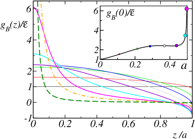
Figure 5: Plots of the solution $g_{B}(z)$ of (39b) as a function of $z/a$, $0<z/a<1$, for values of the void radius (from bottom to top at $z=0$) $a=0.025$ (black), $0.124$ (red), $0.249$ (green), $0.275$ (blue), $0.373$ (gray), $0.435$ (violet), $0.485$ (cyan), $0.498$ (rose), $0.4995$ (orange), $0.499985$ (dark green). Color online. Line and symbol thicknesses increase with $a$.

The solution in terms of $g_{B}$ is as follows. With (39a), $g(z)$ in (37) becomes completely determined in terms of $g_{B}(z)$, $z\in[0,a]$. In the URQ:

$$\varepsilon_{xy}(x,y)=\frac{g_{B}(a)}{2}\left[\theta_{[a,1/2]}(x)+\theta_{[a,1/2]}(y)\right]+\frac{1}{2}[g_{B}(x)\theta_{[0,a]}(x)+g_{B}(y)\theta_{[0,a]}(y)].$$ (42)

The integral equation (39b) admits a continuous solution. Then, $g_{B}$ and in turn $\varepsilon_{xy}$, $\mathbf{u}$ and $\mathbf{u^{*}}$ are continuous, too. The continuity and oddness wrt. $x$ (resp. $y$) of $u^{*}_{x}$ (resp. $u^{*}_{y}$) implies $u_{x}^{*}(0,y)\equiv u_{y}^{*}(x,0)\equiv 0$. Hence, in the URQ:

$$u_{x}^{*}(x,y)=\int_{0}^{y}{\rm d}z\,g(z)-\overline{\varepsilon}y,\qquad u_{y}^{*}(x,y)=u_{x}^{*}(y,x),\qquad(0<x,y<1/2).$$ (43)

These expressions are extended to the unit cell using (92a-92c). From (92d) the transverse components $\sigma_{xx}$ and $\sigma_{yy}$ are odd in $x$ and $y$, so that periodicity requires $\sigma_{xx}(1/2,y)\equiv\sigma_{yy}(x,1/2)\equiv 0$. With $\sigma_{xy}(x,y)=2\lambda\,\varepsilon_{xy}(x,y)$ given by (42), we deduce from stress equilibrium in the URQ of the matrix:

$$\sigma_{xx}(x,y)=\sigma_{yy}(y,x)=\int_{x}^{1/2}{\rm d}\!\,x^{\prime}\,\partial_{y}\sigma_{xy}(x^{\prime},y)=(\lambda/2)(1-2x)g^{\prime}(y).$$ (44)

Then in this region:

$$\sigma_{\text{m,PS}}(x,y)=(\lambda/4)[(1-2x)g^{\prime}(y)\pm(1-2y)g^{\prime}(x)],$$

where the plus (resp. minus) sign applies to $\sigma_{\text{m}}$ (resp. $\sigma_{\text{PS}}$). Hence, because $g_{B}(z)=\text{const.}$ for $z\in[a,1/2]$, the stresses $\sigma_{\text{m}}$ and $\sigma_{\text{PS}}$ vanish in zones (A) of Fig. 2(a). In zones $(B)$, $\sigma_{\text{m}}$ and $\sigma_{\text{PS}}$ are closely related, with:

$$\sigma_{\text{m}}(x,y) = \sigma_{\text{PS}}(x,y)=(\lambda/4)(1-2x)g_{B}^{\prime}(y)\quad\text{ for }\left\{\genfrac{}{}{0.0pt}{1}{a<x<1/2}{0<y<a}\right.,$$ (45a)

$$\sigma_{\text{m}}(x,y) = -\sigma_{\text{PS}}(x,y)=(\lambda/4)(1-2y)g_{B}^{\prime}(x)\quad\text{ for }\left\{\genfrac{}{}{0.0pt}{1}{0<x<a}{a<y<1/2}\right..$$ (45b)

Taking the derivative of (39b) with respect to $z$, we deduce

$$g_{B}^{\prime}(z)=-2z\frac{g_{B}(z)+g_{B}\left(\rho(z)\right)}{\rho(z)[1-2\rho(z)]},$$ (46)

so that $g_{B}^{\prime}(0)=0$. Hence besides zones (A), regions of weak $\sigma_{\text{m}}$ and $\sigma_{\text{PS}}$ lie along the axes $x=0$ or $y=0$, and along the axes $x=\pm 1/2$, $y=\pm 1/2$.

Near the “frontiers” in Fig. 2(a), $\sigma_{\text{m}}$ and $\sigma_{\text{PS}}$ blow up. Indeed, let us focus on the “frontier” $y=a$. From (46), we deduce for $y\lesssim a$

$$g_{B}^{\prime}(y)\simeq-\sqrt{2a}[g_{B}(a)+g_{B}(0)](a-y)^{-1/2},$$ (47)

and the latter stresses behave as $d^{-1/2}$, where $d$ is the distance to the “frontier” line. The variances involving an integral with integrand $\propto\sigma^{2}$, this implies:

$$S^{(1)}(\sigma_{\text{PS}})=S^{(1)}(\sigma_{\text{m}})=\infty.$$ (48)

These divergences are the only ones encountered in the means and variances. The mean stress readily derives from Eqs. (39-40) and (42):

$$\overline{\sigma}=\langle\sigma_{xy}\rangle=8\lambda\left[\int_{0}^{1/2}{\rm d}x\int_{0}^{1/2}{\rm d}y-\int_{0}^{a}{\rm d}x\int_{0}^{\rho(x)}{\rm d}y\right]\varepsilon_{xy}=\lambda\overline{\varepsilon}\left[1+g_{B}(a)/\overline{\varepsilon}\right],$$ (49)

$$\text{The effective shear modulus is therefore}\quad\widetilde{\lambda}=(\lambda/2)\left[1+g_{B}(a)/\overline{\varepsilon}\right].$$ (50)

III.2.2 Moments and effective shear modulus $\widetilde{\lambda}(f)$ in the dilute limit

Series expansions are now carried out for $a\ll 1$. Using the Taylor expansion:

$$g_{B}(az)=\overline{\varepsilon}\sum_{n=0}^{\infty}q_{n}(z)a^{n}\qquad(0<z<1),$$ (51)

we solve Eqn. (39b). Note that $a$ being a parameter, we should have denoted $g_{B}(z)$ by $g_{B}(z;a)$, so that in the above equation, $g_{B}(az)$ would stand for $g_{B}(az;a)$, expanded in powers of $a$. The following recursion is obtained:

$$\frac{q_{n+1}(z)}{2}=q_{n}(1)+\sqrt{1-z^{2}}q_{n}(z)-\int_{\sqrt{1-z^{2}}}^{1}\text{d}\!y\,q_{n}(y),\qquad q_{0}(z)\equiv 1.$$ (52)

Numerically, we find that the series (51) converges for $a<R_{a}\simeq 0.4$. In the convergence region, this solution matches the numerical one obtained in the previous section. We carry out analytically the recursion up to fourth order to estimate $g_{B}(az)/\overline{\varepsilon}$. The integrations are readily performed with a symbolic calculator. Using the result with $z=1$ provides:

$$g_{B}(a)/\overline{\varepsilon}=1-2\pi a^{2}-\frac{64}{3}a^{3}+2(\pi^{2}-6\pi-8)a^{4}+O(a^{5}).$$ (53)

With expansion (53), we find in the dilute limit:

$$\frac{\widetilde{\lambda}}{\lambda}=1-f-\frac{32f^{3/2}}{3\pi^{3/2}}+\left(1-\frac{6}{\pi}-\frac{8}{\pi^{2}}\right)f^{2}+O(f^{5/2}),$$ (54a)

$$M^{(1)}(\varepsilon_{\text{SS}})=1-\frac{32\,f^{3/2}}{3\pi^{3/2}}+O(f^{2}),\quad M^{(2)}(\varepsilon_{\text{SS}})=1+\frac{32\,f^{1/2}}{3\pi^{3/2}}+O(f),$$ (54b)

$$S^{(1)}(\varepsilon_{\text{SS}})=\frac{4\sqrt{2}\,f^{3/4}}{\sqrt{3}\pi^{3/4}}+O(f^{5/4}),\quad S^{(1)}(\sigma_{\text{SS}})=\frac{4\sqrt{2}\,f^{3/4}}{\sqrt{3}\pi^{3/4}}+O(f^{5/4}),$$ (54c)

$$S^{(1)}(\varepsilon_{\text{PS}})=0,\quad S^{(1)}(\sigma_{\text{PS}})=\infty,\quad S^{(1)}(\varepsilon_{\text{m}})=0,\quad S^{(1)}(\sigma_{\text{m}})=\infty.$$ (54d)

A plot of $\widetilde{\lambda}(f)/\lambda$ obtained from the full numerical solution of $g_{B}(z)$ is displayed in Fig. 4. Compared to $\widetilde{\mu}(f)/\mu$, the less singular character of the solution goes along with a harder material at small porosities. But $\widetilde{\lambda}$ falls down to zero much faster than $\widetilde{\mu}$ for higher porosities, excepted near the close-packing threshold.

III.2.3 Scaling in the close packing limit

Day et al. (1992) examined the linear elastic behavior of an isotropic material containing a honeycomb lattice of voids: the effective compressibility and shear moduli (the overall medium is isotropic) vanish as $(f_{c}-f)^{1/2}$ near the void packing threshold. A similar behavior is found here in shear for the anisotropic material.

With the numerical solution of (39b) near $f_{c}$, we observe that the function $g_{B}(z)$ obeys a scaling of the form

$$g_{B}(az)\sim\overline{\varepsilon}(f_{c}-f)^{-1/2}\widetilde{g}\left(z(f_{c}-f)^{-1/2}\right),\quad f\to f_{c},$$ (55)

where the master curve $\widetilde{g}(z)\sim$ const. for $z\ll 1$ and $\widetilde{g}(z)\sim z^{-\tau}$ for $z\gg 1$, where $\tau$ is an exponent close to 2. Fig. 6 provides an illustration for three different values of $a$ near $a_{c}=1/2$.

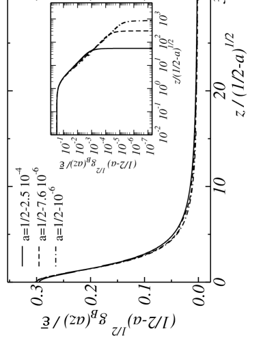
Figure 6: Data collapse illustrating the scaling properties of the function $g_{B}(z)$, for the 3 different values of the radius $a$ indicated in the legend, near the close packing value $a_{c}=1/2$. Inset: same plot in log.-log. scale; the curves break down when $g_{B}(az)$ become negative.

Two consequences are drawn from (55): first, the scaling shows that the strain is concentrated in a band of width $\xi\sim a(f_{c}-f)^{1/2}$, vanishing as the close-packing threshold is approached. Next, relation (55) used at $z=0$ together with (41) and (50) provides near $f_{c}$:

$$\widetilde{\lambda}/\lambda\sim(f_{c}-f)^{1/2},$$ (56a)

as for an isotropic material. The means are readily computed. Moreover, the variances are obtained with the help of the surface integral in the matrix $$\int_{M}{\rm d}x\,{\rm d}y\,\varepsilon_{\text{SS}}^{2}(x,y)=\overline{\varepsilon}^{2}[1+g_{B}(a)/\overline{\varepsilon}]/2$$. The following behaviors near the close-packing threshold ensue:

$$M^{(1)}(\varepsilon_{\text{SS}})\sim\left(f_{c}-f\right)^{1/2},\hfill S^{(1)}(\varepsilon_{\text{SS}})\sim\left(f_{c}-f\right)^{1/4},\hfill S^{(1)}(\sigma_{\text{SS}})\sim\left(f_{c}-f\right)^{-1/4},$$

$$S^{(1)}(\varepsilon_{\text{PS}})=S^{(1)}(\varepsilon_{\text{m}})\equiv 0,\qquad S^{(1)}(\sigma_{\text{PS}})=S^{(1)}(\sigma_{\text{m}})\equiv\infty.$$ (56b)

III.2.4 Distributions and Van Hove singularities

The distributions of the stress fields in the matrix for SS loading, at void concentration $f=0.1$, are displayed in Figs. 7 and 8 as thick solid lines.

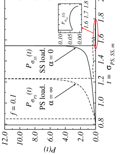
Figure 7: Distributions of the stress components parallel to the applied loading, at void concentration $f=0.1$, in simple shear loading ($\langle\sigma_{\text{SS}}\rangle=1$) with $\alpha=0$ ($P_{\sigma_{\text{SS}}}$, solid), and in pure shear loading ($\langle\sigma_{\text{PS}}\rangle=1$) with $\alpha=\infty$ ($P_{\sigma_{\text{PS}}}$, dashed). Straight vertical lines near $t=0.8$ indicate Dirac components. Inset: magnification of the “foot” in $P_{\sigma_{\text{SS}}}(t)$.

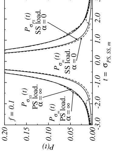
Figure 8: Distributions of the stress components transverse to the applied loading, and of $\sigma_{\text{m}}$, at void concentration $f=0.1$, in simple shear loading ($\langle\sigma_{\text{SS}}\rangle=1$) with $\alpha=0$ ($P_{\sigma_{\text{PS}}}(t)\simeq P_{\sigma_{\text{m}}}(t)$ for $|t|\lesssim 1.5$), and in pure shear loading ($\langle\sigma_{\text{PS}}\rangle=1$) with $\alpha=\infty$ ($P_{\sigma_{\text{SS}}}(t)\simeq P_{\sigma_{\text{m}}}(t)$). Dirac components at $t=0$ should also be present in each of the four sets, due to the void and to zone A, but are omitted for clarity.

In these figures, straight vertical lines represent Dirac components. The distribution $P_{\sigma_{\text{SS}}}(t)$ of the stress “parallel” to the applied loading (Fig. 7) comprises one Dirac component, proportional to $[(1-2a)^{2}/(1-f)]\delta(t-g_{B}(a))$, which represents the contribution of zones (A) of constant $\sigma_{\text{SS}}$, and a divergence followed by a discontinuity of infinite amplitude. The latter comes from the (B) zones. The right “foot” (magnified in the inset) is produced by zones (D) of maximal stress. The distribution has finite support since $\varepsilon_{\text{SS}}$ is bounded. The distributions of the transverse stresses $\sigma_{\text{PS}}$ and of $\sigma_{\text{m}}$ are displayed in Fig. 8. They are even (these fields average to 0). A Dirac contribution at $\sigma=0$ (that of zone (A)) should be present in all plots but is omitted for clarity. The main components blow up at $\sigma=0$ and slowly decrease at $\sigma\to\infty$ (the contribution of zones (B), essentially). The distribution $P_{\sigma_{\text{m}}}$ differs only slightly from $P_{\sigma_{\text{PS}}}$ by the contribution of zones (D), the difference being small at $f=0.1$, for the smallest values of the stress.

The above singular features are understood as follows. Tails of the distributions at high values of the fields are determined by the square-root singularities responsible for the infinite variances (48). Definition (17) of the distribution generates Van Hove singularities (VHS), in the vicinity of values $t=t_{0}$ for which there exists extremal or saddle integration points $\mathbf{x}_{i}$ such that $a(\mathbf{x}_{i})=t_{0}$ and $\partial_{\mathbf{x}}a(\mathbf{x}_{i})=0$. In 2D, depending on the eigenvalues of the matrix $\partial^{2}_{\mathbf{x}\mathbf{x}}a(\mathbf{x}_{i})$ being of same or of opposite signs, the singularity in $P$ is either a discontinuity or a logarithmic divergence (Van Hove, 1953). “Extended” Van Hove singularities (EVHS) (Abrikosov, Campuzano and Gofron, 1993) arise when in addition one or more eigenvalues of $\partial^{2}_{\mathbf{x}\mathbf{x}}a(\mathbf{x}_{i})$ vanish. Consider first the strain distribution. Using (39b), we obtain

$$g_{B}(z)=g_{B}(0)-\frac{\overline{\varepsilon}+g_{B}(a)}{a(1-2a)^{2}}z^{2}+O(z^{4}),$$ (57)

so that in zone (B), for $a<x<1/2$, $0<y<a$,

$$\varepsilon_{xy}(x,y)\simeq\frac{\overline{\varepsilon}+g_{B}(a)}{2(1-2a)}-\frac{\overline{\varepsilon}+g_{B}(a)}{2a(1-2a)^{2}}y^{2}+\ldots,$$ (58)

of the generic type $h(x,y)=h_{0}-h_{1}y^{2}$, $h_{1}>0$. This generates an EVHS near $t=h_{0}=(\overline{\varepsilon}+g_{B}(a))/[2(1-2a)]$, of the form

$$P_{h}(t)\simeq\int\frac{{\rm d}\!x\,{\rm d}\!y}{V}\,\delta\bigl{(}h_{0}-h_{1}y^{2}-t\bigr{)}=\frac{L_{x}}{2V\sqrt{h_{1}}}(h_{0}-t)^{-1/2}\,\theta(h_{0}-t),$$ (59)

where $L_{x}$ is the size of the integration domain on $x$ values. Only values near $y=0$ contribute and the range of integration over $y$ need not be completely specified. The four quadrants account for $L_{x}=2(1-2a)$, so that

$$P_{\varepsilon_{xy}}(t)\simeq\frac{\sqrt{2a}(1-2a)^{2}}{(1-f)\sqrt{\overline{\varepsilon}+g_{B}(a)}}|t-h_{0}|^{-1/2}\theta(h_{0}-t).$$ (60)

Hence the divergence of $P_{\sigma_{\text{SS}}}$, of square-root nature, and the drop of infinite amplitude in Fig. 7 are captured by this approximation, since

$$P_{\sigma_{\text{SS}}}(t)=P_{\varepsilon_{xy}}(t/(2\lambda))/(2\lambda).$$ (61)

Consider next the field distributions $P_{\sigma_{\text{PS}}}(t)$ and $P_{\sigma_{\text{m}}}(t)$ of Fig. 8, and examine the contributions near $t=0$. According to (45) and to the remark following, weak field values lie on the axes $x=0$, $y=0$, $x=\pm 1/2$, $y=\pm 1/2$, where the four points $(x,y)=(\pm 1/2,0)$ and $(x,y)=(0,\pm 1/2)$ contribute most. Focus for instance on $(x,y)=(1/2,0)$. From (45), (46) and (49), and for $y\gtrsim 0$ :

$$\sigma_{\text{m}}(x,y)=\sigma_{\text{PS}}(x,y)\simeq\overline{\sigma}\frac{(1/2-x)y}{a(1-2a)^{2}}.$$ (62)

This is a VHS of type $h(x,y)=h_{1}x^{2}-h_{2}y^{2}$ (rotated 45^o) with $h_{1}$, $h_{2}>0$ so that $P_{h}(t)\sim-\log|t|/(2V\sqrt{h_{1}h_{2}})$ for $t\sim 0$, where $V$ is the integration surface. Using (62), the contributions of the above four points gather into:

$$P_{\sigma_{\text{PS}}}^{(B)}(t)\sim P^{(B)}_{\sigma_{\text{m}}}(t)\sim-\frac{4a(1-2a)^{2}}{\overline{\sigma}(1-f)}\log\left[2(1-2a)^{2}\frac{|t|}{\overline{\sigma}}\right],\qquad t\to 0.$$ (63)

The slowly-decaying tails at high $t$, of $P_{\sigma_{\text{PS}}}(t)$ and $P_{\sigma_{\text{m}}}(t)$ in Fig. 8 are due to singularity (47). Again focusing on the domain $a<x<1/2$, $0<y<a$ in zone (B), and expanding near $y=a$, we obtain from (45) , (46) and (49) :

$$\sigma_{\text{PS}}(x,y)=\frac{\lambda}{4}(1-2x)g_{B}^{\prime}(y)\sim-\frac{\overline{\sigma}\sqrt{2a}}{4(1-2a)}\frac{1-2x}{\sqrt{a-y}},\qquad y\lesssim a.$$

Of type $h(x,y)=-h_{0}(1-2x)/\sqrt{a-y}$, $h_{0}>0$, this expression contributes for

$$\frac{1}{V}\int_{a}^{1/2}{\rm d}x\int^{a}_{0}{\rm d}y\,\delta\bigl{(}h(x,y)-t\bigr{)}=\frac{h_{0}^{2}}{3V}\frac{(1-2a)^{3}}{|t|^{3}}\theta(-t)\theta\left(|t|-\frac{(1-2a)h_{0}}{\sqrt{a}}\right),$$ (64)

where the lower integration bound on $y$ provides the restriction on $|t|$ which delimits the domain of validity of the approximation. Adding contributions from negative values, and multiplying by 4 due to square symmetry leads to:

$$P_{\sigma_{\text{PS}}}^{(B)}(t)\simeq\overline{\sigma}^{2}\frac{a(1-2a)}{6(1-f)}|t|^{-3},\qquad|t|\gg\frac{\overline{\sigma}}{2\sqrt{2}}.$$ (65)

This is only the contribution of $(B)$. The tail should also include a contribution from $(D)$ at high stresses, also decaying as $|t|^{-3}$, but harder to handle due to sign changes at the points $(\pm a,\pm a)$. Other singularities exist which have not been fully investigated: values of $\sigma_{\text{m}}$ around $x,y=\pm a/\sqrt{2}$ produce a singularity in its histogram (extra wings starting at $\sigma_{\text{m}}\simeq\pm 1.7$ with vertical slope, see Fig. 8); moreover, for porosities $f$ higher than 0.6, two inflection points show up in $g_{B}(z)$. They give rise to two local extrema of $\sigma_{\text{m}}$ and $\sigma_{\text{PS}}$ along the cartesian axes zone (B), also producing extra wings of the above type (not shown).

III.3 Equibiaxial loading and limit $\lambda\to 0$

We close the study of the case $\alpha=0$ with equibiaxial loading $\overline{\varepsilon}=\langle\varepsilon_{\text{m}}\rangle\not=0$, $\langle\varepsilon_{\rm PS}\rangle=\langle\varepsilon_{\rm SS}\rangle=0$. The anisotropic limit $\alpha=0$ follows either from letting $\lambda\to 0$, or $\mu\to\infty$, so that two different solutions may a priori arise. Only the case $\lambda\to 0$, with finite $\kappa$, is detailed in this section. Case $\mu\to\infty$ is briefly addressed in Sec. III.4. A method similar to that of Sec. III.1 for PS loading is used. The differences relative to the PS case can be related to the symmetries at play.

III.3.1 Stress and strain fields

The limit $\lambda=0$ under finite macroscopic mean stress requires that $\sigma_{xy}\equiv 0$. Equilibrium and the equivalence of the $Ox$ and $Oy$ axes imply that:

$$\sigma_{xx}(x,y)=g(y),\qquad\sigma_{yy}(x,y)=g(x),$$ (66)

where $g(z)$ is defined on the interval $[-1/2,1/2]$. Similar steps apply as in Sec. III.1. Energy minimization under the same macroscopic stress constraint (20) — with $\overline{\sigma}=\langle\sigma_{\text{m}}\rangle$ replacing $\langle\sigma_{\rm PS}\rangle$, provides $\sigma_{\text{SS}}(x,y)=0$, and

$$\sigma_{\text{m,PS}}(x,y)=\overline{\sigma}\,\frac{\chi(y)\pm\chi(x)}{2(1-2a)},$$ (67)

where the plus (resp. minus) sign applies to $\sigma_{\text{m}}$ (resp. $\sigma_{\text{PS}}$). Associated strains follow from (5). Periodicity conditions on $\mathsf{u}^{*}$ entail:

$$\overline{\sigma}=\frac{2\mu(1-2a)}{m+(1-m)a}\overline{\varepsilon}.$$ (68)

Eqn. (67) reproduces the PS result (21), with the indices PS and m, and with $x$ and $y$, exchanged. Furthermore, the PS and equibiaxial loading modes exchange the parts played by $\kappa$ and $\mu$, which corresponds to interchanging $m\leftrightarrow 1/m$. This circumstance almost allows for a one-to-one mapping of the results of this section onto those of Sec. III.1. For instance in the URQ:

$$\varepsilon_{\text{SS}}=u_{2}\left[\left(x-\frac{1}{2}\right)\delta(y-a)+\left(y-\frac{1}{2}\right)\delta(x-a)\right],\quad u_{2}=\frac{\overline{\varepsilon}}{4}\frac{1+m}{m+(1-m)a}.$$ (69)

Eqn. (69) differs from (28) by a substitution $m\leftrightarrow 1/m$, and by a minus sign due to the difference between (91g) and (93g), or between (91c) and (93c).

III.3.2 Displacement field and singularities

The displacement $\mathbf{u}^{\star}$ in the URQ is such that $u_{x}(x,y)$ is there of the form (30), with $m$ replaced by $1/m$, but with now $u^{*}_{y}(x,y)=u^{*}_{x}(y,x)$. Hence $\mathbf{u}^{\star}$ is again piecewise linear, and tangentially discontinuous at the “frontiers” between (A), (B) and (D). In particular, the jump $[[u^{*}_{x}]]_{y}(x,a)$ along the $y=a$ “frontier” in the URQ is given by (31) with $m$ replaced by $1/m$. With $m=1$, the overall pattern however differs from that of Fig. 3, by the fact that for $\overline{\varepsilon}<0$ (resp. $>0$), the displacements $\mathbf{u}^{\star}$ in all parts of (B) are directed towards the void (resp. outwards), the medium being subjected to compression (resp. extension).

Moreover, owing to symmetry $u^{*}_{y}(x,y)=u^{*}_{x}(y,x)$, the PS mechanism responsible for the formation of the square voids at $(x,y)=(\pm a,\pm a)$ changes into one which induces a compressive singularity near these locations, independently of whether the equibiaxial loading mode is compressive or extensive, over a region of size $\Delta u=\overline{\varepsilon}(m+1)(a/2-1/4)/[m+(1-m)a]$. This is readily seen from the following expression valid in the vicinity of $(x,y)=(a,a)$:

$$\mathbf{u}(x,y)=u_{2}\left[(a+1/2)\left(1,1\right)+(a-1/2)\left(\mathop{\text{sign}}(y-a),\mathop{\text{sign}}(x-a)\right)\right].$$ (70)

The displacement in (D) now reads $\mathbf{u}(x,y)=u_{2}(\mathop{\text{sign}}x,\mathop{\text{sign}}y)$, so that the four “hot spots” $(x,y)=(0,\pm a)$, $(\pm a,0)$ now all undergo a similar local singularity, either of a compressive, or of an extensive nature.

III.3.3 Moments and effective compressibility modulus $\widetilde{\kappa}$

The effective compressibility modulus and the moments are provided by expressions (34a)-(34e), with $\mu$ and $\widetilde{\mu}$ replaced by $\kappa$ and $\widetilde{\kappa}$, with $m$ replaced by $1/m$, and with the indices $PS$ and $m$ interchanged. For definiteness:

$$\frac{\widetilde{\kappa}}{\mu}=\frac{(1-2a)}{m+(1-m)a}=\frac{1}{m}\left[1-\frac{1+m}{m}(f/\pi)^{1/2}+O(f)\right].$$ (71)

Thus, $\widetilde{\kappa}$ possesses a dilute-limit correction $\sim f^{1/2}$ at finite $\kappa$, but blows up as $f^{-1/2}$ in the incompressible limit $m=0$. It decays as $(f_{c}-f)$ near $f_{c}$.

III.4 Equibiaxial loading and limit $\mu\to\infty$

Consider now the limit $\mu\to\infty$, with finite $\lambda$. A finite stress loading is consistent with this limit only if $\varepsilon_{\text{PS}}\equiv 0$. This situation is that of $\alpha=0$ under SS loading, the solution being of like complexity.In particular, for finite compressibility, it is governed by elliptic equations (see Sec. II.4) and is much more complicated than the one of Sec. III.3. Accordingly, we restrict ourselves to the incompressible case $\kappa=\infty$. The solution then simplifies and coincides with that of Sec. III.3 with $m=0$, see (6). Note that $\widetilde{\kappa}$ is infinite, due to $\mu=\infty$.

IV Material with anisotropy ratio $\alpha=\infty$

This section is devoted to the case $\alpha=\infty$, where the material is soft along the diagonals. As Fig. 2b illustrates, the field patterns are now rotated by $45$ degrees. Accordingly, the solutions obtained below could alternatively be derived in a frame where the void lattice is rotated. The corresponding rotation, $\mathcal{R}_{45^{\rm o}}$, would exchange in the matrix $\mathbb{E}^{\rm SS}$ and $\mathbb{E}^{\rm PS}$, and $\lambda$ and $\mu$. In the rotated frame, the following correspondence should then be used

$$\mathcal{R}_{45^{\rm o}}(\text{void lattice})\Leftrightarrow\left\{\alpha\leftrightarrow 1/\alpha,\text{ and }\text{PS loading}\leftrightarrow\text{SS loading},\right\}.$$ (72)

Characteristics for the strain, stress or displacement fields are aligned with the two diagonals of the unit cell (see Sec. II.4). Another difference with the case $\alpha=0$ resides in the appearance of new regions in the matrix, denoted by (C) in the figure, where the (B) bands cross, with no holes in it.

IV.1 Loading in simple shear

We impose $\mu=0$, $\alpha=\infty$ and consider SS loading conditions. Due to (5), $\mu=0$ implies $\sigma_{\text{PS}}=(\sigma_{xx}-\sigma_{yy})/2\equiv 0$, so that $\sigma_{xx}(x,y)=\sigma_{yy}(x,y)\equiv s(x,y)$, an unknown function. Stress equilibrium implies $\partial^{2}s$ $/\partial x^{2}$ $-$ $\partial^{2}s$ $/\partial y^{2}$ $=$ $0$. Using the identities in Appendix A, we deduce that $s(x,y)=[g(x-y)-g(x+y)]/2$, where $g$ is an unknown, even, 1-periodic function. The stress $\sigma_{xy}=\sigma_{\text{SS}}$ stems from integrating the stress equilibrium equations. The integration constant is zero, since $\mathbf{\sigma}=0$ in the void. Eventually, with $g(0)=0$,

$$\sigma_{\text{SS}}(x,y)=[g(x-y)+g(x+y)]/2,\qquad\sigma_{\text{m}}(x,y)=[g(x-y)-g(x+y)]/2.$$ (73)

Due to the void one has, along the main diagonal, $\sigma_{\text{m}}(x,x)=-g(2x)/2\equiv 0$ for $x<a/\sqrt{2}$. Hence $g(z)\equiv 0$ on $[-\sqrt{2}a,\sqrt{2}a]$. In turn, stresses (73) vanish in the whole square made of zones (V) and (D) in Fig. 2(b). Due to 1-periodicity and to $g$ being even, the stress pattern possesses a mirror symmetry with respect to the dashed lines of Fig. 2(b). Its fundamental unit cell is therefore the gray square delimited by them. Symmetry (72) makes this case tantamount to the PS case of Sec. III.1 with $\alpha=0$ and $\lambda=0$, with a cell size diminished by a factor $1/\sqrt{2}$ at constant pore radius $a$ and, consequently, with a porosity twice bigger. Effective moduli and moments are then obtained from expressions (34) of Sec. III.1, with $\mu$ and $\widetilde{\mu}$ replaced by $\lambda$ and $\widetilde{\lambda}$, with $m$ replaced by $\ell$, with the subscripts SS and PS exchanged, and with $a$ replaced by $\sqrt{2}a$. Deformation in the non-voided crossing zones (C) of zero stress is understood as follows. The obtained solutions for the displacement and strain fields in the (D) zones are trivially continued to the voided zone (V). These admissible continuations are non-physical except on the void boundary. However, the above symmetry considerations make clear that, modulo an appropriate translation, these continuations also provide the physical deformation fields in (C).

Mutatis mutandis, the obtained expressions for the fields and the moduli are valid only up to $f=f_{c}^{(1)}=\pi/8$, due to the rescaling of $a$. This concentration acts as a “mechanically driven percolation” threshold, at half the close-packing value. It corresponds to the configuration where the summits (D) in Fig. 2b come into contact with the cell boundaries. Then, (A) and (B) vanish, leaving only (C) and (D) for $f$ up to $f_{c}=\pi/4$. Thus, for $f>f_{c}^{(1)}$, $\sigma_{\text{SS}}$ vanishes in the matrix. The stress $\varepsilon_{\text{SS}}$ also vanishes, so that strain only takes place along the void boundaries. Consequently, $\widetilde{\lambda}$ vanishes for $f\geq f_{c}^{(1)}$ and the fields are such that: $M^{(1)}(\varepsilon_{\text{SS}})=0$, $M^{(1)}(\varepsilon_{\text{PS}})=1/f$, $S^{(1)}(\varepsilon_{\text{SS}})=0$. Fig. 9 displays $\widetilde{\lambda}(f)/\lambda$ vs. $f$. Except for the threshold, the curve is alike that of $\widetilde{\mu}(f)/\mu$ in Fig. 4.

In words, we just showed that special field configurations in linear anisotropic periodic media can lower the geometric “percolation” threshold of the porous material (i.e. the close-packing threshold, for a periodic pore lattice) into one determined by effective “porous” zones (as far as they undergo vanishing stresses) at intersections of void-generated stress bands. This is unusual: for instance in homogenization methods, percolation-like thresholds are usually thought (or found) to be independent of the constitutive law.

IV.2 Loading in pure shear (incompressible case only)

In the case $\alpha=\infty$ with $\lambda=\infty$ and $\mu$ finite, under PS loading, the solution has the pattern of Fig. 2(b). It is of the type studied in Sec.III.2, at least for $f$ up to $f_{c}^{(1)}=\pi/8$. For $f>f_{c}^{(1)}$ the problem becomes more involved due to a complex geometry, and has not been investigated in full. Only the range $f<f_{c}^{(1)}$ is discussed hereafter.

IV.2.1 Displacements, strain and stress fields

The solution obeys $\varepsilon_{\text{SS}}=\varepsilon_{xy}\equiv 0$, and the incompressibility constraint $\varepsilon_{xx}$ $+$ $\varepsilon_{yy}$ $\equiv$ $0$. Expressed in terms of $u^{*}_{x}$, $u^{*}_{y}$, such that $u^{*}_{x}(0,y)$ $=$ $u^{*}_{y}(x,0)$ $\equiv$ $0$ as implied by (91a) and (91b), these equations entail with the help of (91c):

$$u^{*}_{x}(x,y)=[G(x+y)+G(x-y)]/2,\quad u^{*}_{y}(x,y)=[-G(x+y)+G(x-y)]/2,$$ (74)

and eventually with $g(z)=G^{\prime}(z)$ an even and 1-periodic function:

$$\varepsilon_{\rm PS}(x,y)=\left[g(y-x)+g(x+y)\right]/2.$$ (75)

Introducing the 45${}^{\textnormal{o}}$ counterclockwise-rotated coordinates $x^{\prime}=(y+x)/\sqrt{2}$ and $y^{\prime}=(y-x)/\sqrt{2}$, such that $-1/(2\sqrt{2})\leq x^{\prime},y^{\prime}\leq 1/(2\sqrt{2})$, functions $g_{\text{B}}$ and $g_{\text{A}}$ are introduced, such that

$$g(\sqrt{2}x^{\prime})=g_{\text{B}}(x^{\prime})\,\theta_{[0,a]}(x^{\prime})+g_{\text{A}}(x^{\prime})\,\theta_{[a,1/(2\sqrt{2})]}(x^{\prime}).$$ (76)

The total elastic energy in the unit cell (7) is provided by the integral:

$$(1-f)\langle w^{(1)}\rangle_{(1)}=2\mu\int_{M}{\rm d}^{2}x\,\varepsilon_{\text{PS}}^{2}=2\mu\biggl{\{}\qquad 2\int_{[-1/(2\sqrt{2}),1/(2\sqrt{2})]^{2}\phantom{\biggl{(}}}{\rm d}x^{\prime}{\rm d}y^{\prime}-\int_{V}{\rm d}x^{\prime}{\rm d}y^{\prime}\biggr{\}}\varepsilon_{\text{PS}}^{2}(x^{\prime},y^{\prime}).$$ (77)

One extra contribution of the void $V$ (of no elastic energy) has been subtracted from the contribution of the gray square in Fig. 2(b), counted twice. Anticipating on the fact that on its interval of definition $g_{\text{A}}(z)\equiv g_{\text{B}}(a)$, as in Sec. III.2.1, the energy (7) is functionally minimized under the constraint:

$$\overline{\varepsilon}=\left\langle\varepsilon_{\text{PS}}\right\rangle=2\sqrt{2}\int_{0}^{a}g_{\text{B}}(y){\,{\rm d}y}+\left(1-2\sqrt{2}a\right)g_{\text{B}}(a),$$ (78)

This average is computed on one gray square, with the strain field (75) continued inside the void. Setting $\rho(z)\equiv\sqrt{a^{2}-z^{2}}$, an integral equation results:

$$\sqrt{2}\int_{0}^{\rho(z)}g_{\text{B}}(y){\,{\rm d}y}=\left[1-\sqrt{2}\rho(z)\right]g_{\text{B}}(z)-g_{\text{B}}(a),\qquad z\in[0,a].$$ (79)

Its solution is obtained following Sec. III.2.1. In particular, with $z=0$ and (78):

$$g_{\text{B}}(0)=\frac{\overline{\varepsilon}+(1+2\sqrt{2}a)g_{\text{B}}(a)}{2(1-\sqrt{2}a)}.$$ (80)

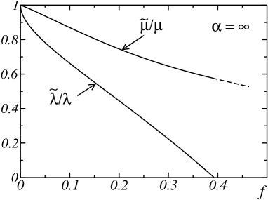
Figure 9: Normalized shear effective moduli $\widetilde{\mu}/\mu$ and $\widetilde{\lambda}/\lambda$ vs. void concentration $f$, for an incompressible matrix with anisotropy ratio $\alpha=\infty$. The curve for $\widetilde{\mu}/\mu$ is computed up to $f=\pi/8$ only. Modulus $\widetilde{\lambda}$ vanishes at $f_{c}^{(1)}=\pi/8\simeq 0.39$, half the close packing threshold value.

The displacement is everywhere continuous. The stress $\sigma_{\text{PS}}$ is deduced from (75) and from $\sigma_{\text{PS}}=2\mu\varepsilon_{\text{PS}}$ in the matrix, with $\sigma_{\text{PS}}=0$ in the voids. The transverse components $\sigma_{\text{m}}$, $\sigma_{\text{SS}}$ are computed analogously to (44), with integrations and differentiations carried out over $x^{\prime}$ and $y^{\prime}$. Stress equilibrium provides:

$$\partial_{x^{\prime}}\,\sigma_{\text{PS}}=\partial_{y^{\prime}}(\sigma_{\text{m}}-\sigma_{\text{SS}}),\qquad\partial_{y^{\prime}}\,\sigma_{\text{PS}}=\partial_{x^{\prime}}(\sigma_{\text{m}}+\sigma_{\text{SS}}).$$ (81)

Due to symmetry, $\sigma_{\text{m}}(x,x)=\sigma_{\text{SS}}(x,x)\equiv 0$ and $\sigma_{\text{m}}(x,1-x)=\sigma_{\text{SS}}(x,1-x)\equiv 0$, so that with $0<x,y<1$ in the matrix (for convenience, a unit cell translated by a vector $\mathbf{t}=(1/2,1/2)$ is considered):

$$\sigma_{\text{m,SS}}(x^{\prime},y^{\prime})=(1/2)\int_{1/\sqrt{2}}^{x^{\prime}}\!\!\!{\rm d}z\,\partial_{y^{\prime}}\sigma_{\text{PS}}(z,y^{\prime})\pm(1/2)\int_{0}^{y^{\prime}}\!\!\!{\rm d}z\,\partial_{x^{\prime}}\sigma_{\text{PS}}(x^{\prime},z),$$ (82)

The plus (resp. minus) sign applies to $\sigma_{m}$ (resp. $\sigma_{\text{SS}}$). Then, in the matrix:

$$\sigma_{\text{m,SS}}(x,y)=\frac{\mu}{2}\left[(x+y-1)g^{\prime}\left(y-x\right)\pm(y-x)g^{\prime}\left(x+y-1\right)\right]$$ (83)

for $0<x,y<1$. For $z$ in $[0,a\sqrt{2}]$, the derivative $g^{\prime}$ reduces to $g^{\prime}(z)$ $=$ $g^{\prime}_{\text{B}}(z/\sqrt{2})$ $/\sqrt{2}$ where $g^{\prime}_{B}$ is the derivative of $g_{B}$. The stress and strain singularities are qualitatively the same as in the $\alpha=0$, SS loading case. In particular, from (79), $g_{B}(z)\simeq g_{B}(a)+2\sqrt{a}[g_{B}(0)+g_{B}(a)]|a-z|^{1/2}$, for $z\lesssim a$, so that $\sigma_{\text{PS}}$ blows up along the “frontiers” of (A), (B), (C) and (D) as $d^{-1/2}$ where $d$ is the distance to the “frontier”.

IV.2.2 Moments and effective modulus $\widetilde{\mu}(f)$ in the dilute limit

Expanding $g_{B}(z)$ in powers of $a$, we obtain:

$$g_{B}(a)/\overline{\varepsilon}=1-2\pi a^{2}-\frac{32\sqrt{2}}{3}a^{3}+\left[(5/2)\pi^{2}-6\pi-8\right]a^{4}+O(a^{5}).$$ (84)

Dilute expansions in $f$ for the effective modulus and the moments ensue:

$$\frac{\widetilde{\mu}}{\mu}=1-f-\frac{32}{3\sqrt{2}\pi^{3/2}}f^{3/2}+\left(1-\frac{3}{\pi}-\frac{4}{\pi^{2}}\right)f^{2}+O(f^{5/2}),$$ (85a)

$$M^{(1)}(\varepsilon_{\text{PS}})=1-\frac{32f^{3/2}}{3\sqrt{2}\pi^{3/2}}+O(f^{2}),\quad M^{(2)}(\varepsilon_{\text{PS}})=1+\frac{32f^{1/2}}{3\sqrt{2}\pi^{3/2}}+O(f),$$ (85b)

$$S^{(1)}(\varepsilon_{\text{PS}})=\frac{4\,2^{1/4}f^{3/4}}{\sqrt{3}\pi^{3/4}}+O(f^{5/4}),\quad S^{(1)}(\sigma_{\text{PS}})=\frac{4\,2^{1/4}f^{3/4}}{\sqrt{3}\pi^{3/4}}+O(f^{5/4}),$$ (85c)

$$S^{(1)}(\varepsilon_{\text{SS}})=0,\quad S^{(1)}(\sigma_{\text{SS}})=\infty;\quad S^{(1)}(\varepsilon_{\text{m}})=0,\quad S^{(1)}(\sigma_{\text{m}})=\infty.$$ (85d)

In the range $0<f<\pi/8$, $\widetilde{\mu}(f)$ is computed from a numerical solution of (79). Contrarily to the SS case where $\widetilde{\lambda}(f)$ vanishes at $\pi/4$, no  “mechanically driven percolation” is found here, since the zones (C) where bands cross are not zones of vanishing stress. Regular close packing behavior must occur at $f_{c}=\pi/4$.

IV.2.3 Distributions

Field distributions are studied as in Sec. III.2.4. Quite similar features are observed, summarized hereafter, along with some differences. The density $P_{\varepsilon_{\text{PS}}}$ is non-symmetric, and supported by the interval $[g_{\text{B}}(a),g_{\text{B}}(0)]$. A rescaling similar to (61), using $\mu$ instead of $\lambda$, provides $P_{\sigma_{\text{PS}}}$, plotted in Fig. 7 (dashed curve). Due to the gradient of $\varepsilon_{\text{PS}}(x,y)$ vanishing along the lines $y=\pm x$, where the field is maximum in (B), $P_{\varepsilon_{\text{PS}}}(t)$ blows up as $|t-t_{0}|^{-1/2}$ at $t_{0}=[g_{\text{B}}(a)+g_{\text{B}}(0)]/2$. A notable difference with the case $\alpha=0$ lies in the existence of the extended “foot” on the right side of $P_{\sigma_{\text{PS}}}$. It ends with a discontinuous VHS of finite amplitude, due to the maximum strain field value, $\max\varepsilon_{\text{PS}}=g_{\text{B}}(0)$, being reached at $(x,y)=(\pm 1/2,\pm 1/2)$, in (C). In the case $\alpha=0$, $\sigma=0$ in this zone. The discontinuity is computed by remarking that according to (75), (76) and to a Taylor expansion of $g_{B}(z)$ at $z=0$, the strain field $\varepsilon_{\text{PS}}$ at points $(x,y)=(\pm 1/2,\pm 1/2)$ is a quadratic function with negative eigenvalues. Furthermore, a field $h(x,y)\simeq-(h_{1}x^{2}+h_{2}y^{2})$ with $h_{1}$, $h_{2}>0$, on a domain $V$, produces in $P_{h}(t)$ a jump at the origin $[[P_{h}(0)]]=-\pi/(4\sqrt{h_{1}h_{2}}V)$.

Densities $P_{\sigma_{\text{m}}}$, $P_{\sigma_{\text{SS}}}$ stem from Eqn. (83). They blow up at the origin due to points of vanishing derivatives $\partial_{x}\sigma_{\text{m,SS}}$, $\partial_{y}\sigma_{\text{m,SS}}$. According to (83) this happens for $(x,y)=(1/2,1/2)$. In the vicinity of this point, the expansion of $\sigma_{\text{m}}$ is quadratic of a regular type and leads to logarithmic divergent VHS of $P_{\sigma_{\text{m}}}(t)$ at the origin. On the other hand, $\sigma_{\text{SS}}(x,y)$ is of an unusual cubic form:

$$\sigma_{\text{SS}}(x,y)\propto(y-x)(x+y-1)\left(x-1/2\right).$$ (86)

This generates a singular contribution to $P_{\sigma_{\text{SS}}}(t)$ at the origin, of a type not previously encountered: indeed, the distribution $P_{h}(t)$ of a function $h(x,y)=h_{0}(y^{2}-x^{2})x$ behaves near $t=0$ as $|t|^{-1/3}$. Finally, the tails of $P_{\sigma_{\text{m}}}(t)$, $P_{\sigma_{\text{SS}}}(t)$ when $|t|\to\infty$ decay unsurprisingly as $|t|^{-3}$, due to the blowing-up of the concerned stress components along the “frontiers” between zones (A), (B), (C), (D) as an inverse square root of the distance.

IV.3 Equibiaxial loading

We consider here the limit $\alpha=\lambda/\mu=\infty$, achieved by taking $\mu\to 0$, under equibiaxial loading. The limit $\lambda\to\infty$ is not dealt with for the same reason as in Sec. III.4. Moderate porosities $f<f_{c}$ are assumed. The method used for the case $\alpha=0$ is applied to the void lattice rotated by 45 degrees, and undergoing symmetry (72). With $a_{s}=\sqrt{2}a$ and with the rotated coordinates $x^{\prime}=(y+x)/\sqrt{2}$ and $y^{\prime}=(y-x)/\sqrt{2}$, the stresses are $\sigma_{\text{PS}}(x,y)\equiv 0$, and

$$\sigma_{\text{m,SS}}(x,y)=\overline{\sigma}[\chi(y^{\prime})\pm\chi(x^{\prime})]/[2(1-2a_{s})],$$ (87)

in the rotated gray domain of Fig. 2b. Hence, with $\varpi\equiv(\overline{\varepsilon}/2)/[\ell+(1-\ell)a_{s}]$,

$$\varepsilon_{\text{m}}(x,y)=\ell\,\varpi\,[\chi(y^{\prime})+\chi(x^{\prime})],\quad\varepsilon_{\text{SS}}(x,y)=\varpi\,[\chi(y^{\prime})-\chi(x^{\prime})].$$ (88)

Likewise, the PS component of the strain field takes the Dirac-localized form for $x^{\prime},y^{\prime}$ in the URQ of the rotated gray square:

$$\varepsilon_{\text{PS}}(x,y)=(1+\ell)\varpi\left[\left(x^{\prime}-\frac{1}{\sqrt{2}}\right)\delta(y^{\prime}+a)+\left(y^{\prime}-\frac{1}{\sqrt{2}}\right)\delta(x^{\prime}-a)\right].$$ (89)

Then, the following effective compressibility modulus is obtained:

$$\frac{\widetilde{\kappa}}{\lambda}=\frac{1-2a_{s}}{\ell+(1-\ell)a_{s}}.$$ (90)

“Mechanically driven percolation” is again observed here. The moments of the fields are read from expressions (34b)–(34e), by carrying out the following substitutions: (i) replace $a$ by $a_{s}$; (ii) replace $m$ by $1/\ell$; (iii) replace index PS by index m; (iv) replace index m by index SS; (v) replace index SS by index PS.

V Discussion and conclusion

Two essentially different types of solutions, in an infinitely anisotropic linear elastic medium containing a periodic distribution of voids, have been exhibited. The anisotropy directions of the matrix — a “hard” one and a “soft” one — being aligned with the lattice directions, the fields are arranged in patterns of bands.

On the one hand, for shear loading along a “hard” direction, the following observations were made: ($i$) the “parallel” components of the stress and strain are discontinuous, piecewise constant, with a band width of one pore diameter; ($ii$) the deformation pattern has a “block sliding” structure; ($iii$) the shear strain orthogonal to the loading has infinite variance, being localized as Dirac distributions along the band “frontiers”, which are tangent to the voids (with jumps at the tangency points); ($iv$) the “perpendicular” component of the stress is zero. The presence of discontinuities in the tangential component of the displacement field is analogous to similar observation in ideal plasticity, including the Hencky plasticity model (Suquet, 1981). Moreover, in situations where the bands cross, the medium develops fictitious porous zones of zero parallel stress which lower the close packing threshold. Also, a first-order correction $\sim f^{1/2}$ is induced in the effective shear modulus. The latter decays linearly with the void concentration near the close packing threshold.

On the other hand, for loading along a “soft” direction, another type of solution is produced when the problem is hyperbolic, i.e. assumed to be incompressible. In this case, the following observations were made: ($i$) the strains are continuous everywhere; ($ii$) the leading order correction to the effective shear modulus in the loading direction is now $\propto f$, i.e. less sensitive to increasing void concentration for small concentrations; ($iii$) the variances of the “parallel” stress and strain in the matrix are $\propto f^{3/4}$ and are again less sensitive to increasing void concentration; ($iv$) the parallel strain enjoys scaling properties near the close-packing threshold $f_{c}$, operating within a band of width $\xi\sim a(f_{c}-f)^{1/2}$, and becomes fully localized only for $f$ near $f_{c}$. This situation is at best one of “very soft” void-induced strain localization. However, stresses accumulate in the “hard” directions (transverse and equibiaxial) and blow up along the “frontiers” of the field pattern as the inverse square root of the distance (the corresponding strains being zero). This particular stress localization configuration may be relevant to strain-locking materials, such as the shape-memory polycrystals that have been considered recently by Bhattacharya and Suquet (2005) and Chenchiah and Bhattacharya (2005).

In conclusion, situations responsible for fractional exponents showing up in anisotropic linear theories, of relevance to non-linear homogenization methods, have been clarified. Comparisons with fully numerical results at moderate anisotropies, and for isotropic viscoplasticity, will be presented elsewhere (Willot et al., 2007). As a final remark, the fact that strong singularities are found (isolated points of matter overlapping or of matter separation) in one case is obviously of relevance for breakdown studies (e.g., in brittle materials), since these points may act as initiators. This may suggest that mechanically sounder solutions could be looked for in a large deformation framework. However, in view of our more modest aim to help better understand possible hallmarks of localization in non-linear homogenization theories, the model considered here is adequate.

VI Acknowledgements

The authors wish to thank the anonymous referee for remarks pertaining to the interpretation of the solutions in terms of characteristics. The work of P.P.C. was supported in part by the N.S.F. through Grant OISE-02-31867 in the context of collaborative project with the C.N.R.S.

Appendix A Symmetry properties for the strain, stress and displacement fields

Since the periodic anisotropic medium obeys the symmetries of the square, the symmetries of the displacement $\mathbf{u}$ are determined by the applied loading. They are easily deduced from Figs. 1(b) in simple shear and 1(c) in pure shear, and from an obvious flow pattern in equibiaxial loading. Differentiations wrt. $x$ and $y$ provides those enjoyed by $\varepsilon_{ij}$. The symmetry group of the constitutive law carries them unchanged over $\sigma_{ij}$. For $\mathbf{v}=\mathbf{u}$ or $\mathbf{u}^{*}$ and for $\mathsf{a}=\mbox{\boldmath$\varepsilon$}$ or $\sigma$:

• In PS loading:

  $$v_{x}(x,y) = -v_{x}(-x,y)=v_{x}(x,-y),$$ (91a)

  $$v_{y}(x,y) = v_{y}(-x,y)=-v_{y}(x,-y),$$ (91b)

  $$v_{x}(x,y) = -v_{y}(y,x),$$ (91c)

  $$a_{ii}(x,y) = a_{ii}(-x,y)=a_{ii}(x,-y),\qquad i=x,y,$$ (91d)

  $$a_{xx}(x,y) = -a_{yy}(y,x),$$ (91e)

  $$a_{xy}(x,y) = -a_{xy}(-x,y)=-a_{xy}(x,-y),$$ (91f)

  $$a_{xy}(x,y) = -a_{xy}(y,x);$$ (91g)

• In SS loading:

  $$v_{x}(x,y) = v_{x}(-x,y)=-v_{x}(x,-y),$$ (92a)

  $$v_{y}(x,y) = -v_{y}(-x,y)=v_{y}(x,-y),$$ (92b)

  $$v_{x}(x,y) = v_{y}(y,x),$$ (92c)

  $$a_{ii}(x,y) = -a_{ii}(-x,y)=-a_{ii}(x,-y),\qquad i=x,y,$$ (92d)

  $$a_{xx}(x,y) = a_{yy}(y,x),$$ (92e)

  $$a_{xy}(x,y) = a_{xy}(-x,y)=a_{xy}(x,-y),$$ (92f)

  $$a_{xy}(x,y) = a_{xy}(y,x);$$ (92g)

• In equibiaxial loading:

  $$v_{x}(x,y) = -v_{x}(-x,y)=v_{x}(x,-y),$$ (93a)

  $$v_{y}(x,y) = v_{y}(-x,y)=-v_{y}(x,-y),$$ (93b)

  $$v_{x}(x,y) = v_{y}(y,x),$$ (93c)

  $$a_{ii}(x,y) = a_{ii}(-x,y)=a_{ii}(x,-y),\qquad i=x,y,$$ (93d)

  $$a_{xx}(x,y) = a_{yy}(y,x),$$ (93e)

  $$a_{xy}(x,y) = -a_{xy}(-x,y)=-a_{xy}(x,-y),$$ (93f)

  $$a_{xy}(x,y) = a_{xy}(y,x).$$ (93g)

References

- (1) Abrikosov, A.A., Campuzano, J.C., Gofron, K., 1993. Experimentally observed extended saddle point singularity in the energy spectrum of YBa2Cu4O6.9 and YBa2Cu4O8 and some of the consequences, Physica C: Superconductivity 214 (1-2), 73–79.
- (2) Bhattacharya, K. and Suquet, P. M., 2005. A model problem concerning recoverable strains of shape memory polycrystals. Proc. R. Soc. Lond. A 461, 2797–2816.
- (3) Chenchiah, I.V. and Bhattacharya, K., 2005. Examples of non-linear homogenization involving degenerate energies. I. Plane strain. Proc. R. Soc. A 461, 3681–3703.
- (4) Cule, D., Torquato, S., 1998. Electric field distribution in composite media. Phys. Rev. B 58, 11829–11832.
- (5) Day, A.R., Snyder K.A., Garboczi E.J., Thorpe M.F., 1992. The elastic moduli of a sheet containing circular holes. J. Mech. Phys. Solids 40, 1031–1051.
- (6) Drucker, D.C., 1966. The continuuum theory of plasticity on the macroscale and the microscale. J. Mater. 1, 873–910.
- (7) Ekeland, I. and Temam, R., 1974. Analyse convexe et problèmes variationnels. Dunod, Paris.
- (8) Francescato, P., Pastor, J., 1998. Résistance de plaques multiperforées : comparaison calcul-experience. Rev. Eur. Éléments Finis 7, 421–437.
- (9) Francescato, P., Pastor, J., Riveill-Reydet, B., 2004. Ductile failure of cylindrically porous materials. Part I: plane stress problem and experimental results. Eur. J. Mech. A/Solids 23, 181–190.
- (10) Kachanov, L.M., 1974. Fundamentals of the theory of plasticity. Mir Publishers, Moscow.
- (11) Lahellec, N., Suquet, P., 2004. Nonlinear composites: a linearization procedure exact to second order in contrast and for which the strain-energy and affine formulations coincide. C.R. Mécanique 332, 693–700.
- (12) McPhedran, R.C. and Movchan, A.B., 1994. The Rayleigh multipole method for linear elasticity. J. Mech. Phys. Solids 42, 71 l–727.
- (13) Masson, R., Bornert, M., Suquet, P., Zaoui, A., 2000. An affine formulation for the prediction of the effective properties of nonlinear composites and polycrystals. J. Mech. Phys. Solids. 48, 1203–1227.
- (14) M. Otto, J.-P. Bouchaud, P. Claudin, J. E. S. Socolar, 2003. Anisotropy in granular media: Classical elasticity and directed-force chain network. Phys. Rev. E 67, 031302.
- (15) Pastor, J., Ponte Castañeda, P., 2002. Yield criteria for porous media in plane strain: second-order estimates versus numerical results. C.R. Mécanique 330, 741–747.
- (16) Pellegrini, Y.P., 2001. Self-consistent effective-medium approximation for strongly non-linear media. Phys. Rev. B 64, 134211.
- (17) Ponte Castañeda, P., 1991. The effective mechanical properties of nonlinear isotropic composites. J. Mech. Phys. Solids. 39 (1), 45–71.
- (18) Ponte Castañeda, P., DeBotton, G., Li, G., 1992. Effective properties on nonlinear inhomogeneous dielectrics. Phys. Rev. B 46 (8), 4387–4394.
- (19) Ponte Castañeda, P., 1996. Exact second-order estimates for the effective mechanical properties of nonlinear composite materials. J. Mech. Phys. Solids 44, 827–862.
- (20) Ponte Castañeda, P., 2001. Second-order theory for nonlinear dielectric composites incorporating field fluctuations. Phys. Rev. B 64, 214205.
- (21) Ponte Castañeda, P., 2002. Second-order homogenization estimates for nonlinear composites incorporating field fluctuations. I Theory. J. Mech. Phys. Solids 50, 737–757, and Part II -Applications, ibid., 759–782.
- (22) Suquet, P.M., 1981. Sur les équations de la plasticité: existence et régularité des solutions. J. Mécanique 20, 3–39.
- (23) Torquato, S., 2002. Random Heterogeneous Materials: microstructure and macroscopic properties. Springer, New York.
- (24) Van Hove, L., 1953. The occurrence of singularities in the elastic frequency distribution of a crystal. Phys. Rev. 89 (6), 1189–1193.
- (25) Willis, J. R., 1986. Variational estimates for the overall response of an inhomogeneous nonlinear dielectric. In: Homogenization and Effective Moduli of Materials and Media, J.L. Ericksen et al eds., Springer-Verlag, New-York, 247–263.
- (26) Willot, F., Pellegrini, Y.-P., Idiart, M., Ponte Castañeda, P., 2007. In preparation.
- (27) Zachmanoglou, E. C., Thoe, D.W., 1986. Introduction to partial differential equations. Dover, New York.
- (28) Zeng, X.C.,Bergman, D.J., Hui, P.M., Stroud, D., 1988. Effective-medium theory for weakly non-linear composites. Phys. Rev. B 38, 10970–10973.