Two-fluid model of the Truncated Euler’s Equations

Abstract

A phenomenological two-fluid model of the (time-reversible) spectrally-truncated $3D$ Euler equation is proposed. The thermalized small scales are first shown to be quasi-normal. The effective viscosity and thermal diffusion are then determined, using EDQNM closure and Monte-Carlo numerical computations. Finally, the model is validated by comparing its dynamics with that of the original truncated Euler equation.

1 Introduction

It is well-known that the (inviscid and conservative) truncated Euler equation admits absolute equilibrium solutions with Gaussian statistics, equipartition of kinetic energy among all Fourier modes and thus an energy spectrum $E(k)\sim k^{2}$ [1]. Recently, Cichowlas et al. [2, 3] observed that the Euler equation, with a very large (several hundreds) spectral truncation wavenumber $k_{\rm max}$, has long-lasting transients which behave just as those of high-Reynolds number viscous flow; in particular they found an approximately $k^{-5/3}$ inertial range followed by a dissipative range. How is such a behavior possible? It was found that the highest-$k$ modes thermalize at first, displaying a $k^{2}$ spectrum. Progressively the thermalized region extends to lower and lower wavenumbers, eventually covering the whole range of available modes. At intermediate times, when the thermalized regime only extends over the highest wavenumbers, it acts as a thermostat that pumps out the energy of larger-scale modes. Note that similar $k^{-5/3}$/ $k^{2}$ spectra have already been discussed in the wave turbulence literature (e.g.,[4]) and were more recently obtained, within a simple differential closure, in connection with the Leith model of hydrodynamic turbulence [5].

The purpose of the present work is to build a quantitative two-fluid model for the relaxation of the $3D$ Euler equation. In section 2, after a brief recall of basic definitions, the statistics of the thermalized small scales are studied during relaxation. They are shown to be quasi-normal. Our new two-fluid model, involving both an effective viscosity and a thermal diffusion, is introduced in section 3. The effective diffusion laws are then determined, using an EDQNM closure prediction and direct Monte-Carlo computations. The model is then validated by comparing its predictions with the behavior of the original truncated Euler equation. Finally section 4 is our conclusion.

2 Relaxation dynamics of truncated Euler equations

2.1 Basic definitions

The truncated Euler equations (1) are classically obtained [1] by performing a Galerkin truncation ($\hat{v}(k)=0$ for $sup_{\alpha}|k_{\alpha}|>k_{max}$) on the Fourier transform ${\bf v}({\bf x},t)=\sum{\bf\hat{v}}({\bf k},t)e^{i{\bf k}\cdot{\bf x}}$ of a spatially periodic velocity field obeying the (unit density) three-dimensional incompressible Euler equations, ${\partial_{t}{\bf v}}+({\bf v}\cdot\nabla){\bf v}=-\nabla p~{},$ $\nabla\cdot{\bf v}=0$. This procedure yields the following finite system of ordinary differentials equations for the complex variables ${\bf\hat{v}}({\bf k})$ (${\bf k}$ is a 3 D vector of relative integers $(k_{1},k_{2},k_{3})$ satisfying $\sup_{\alpha}|k_{\alpha}|\leq k_{\rm max}$)

$${\partial_{t}{\hat{v}}_{\alpha}({\bf k},t)}=-\frac{i}{2}{\mathcal{P}}_{\alpha\beta\gamma}({\bf k})\sum_{\bf p}{\hat{v}}_{\beta}({\bf p},t){\hat{v}}_{\gamma}({\bf k-p},t)$$ (1)

where ${\mathcal{P}}_{\alpha\beta\gamma}=k_{\beta}P_{\alpha\gamma}+k_{\gamma}P_{\alpha\beta}$ with $P_{\alpha\beta}=\delta_{\alpha\beta}-k_{\alpha}k_{\beta}/k^{2}$ and the convolution in (1) is truncated to $\sup_{\alpha}|k_{\alpha}|\leq k_{\rm max}$, $\sup_{\alpha}|p_{\alpha}|\leq k_{\rm max}$ and $\sup_{\alpha}|k_{\alpha}-p_{\alpha}|\leq k_{\rm max}$.

This time-reversible system exactly conserves the kinetic energy $E=\sum_{k}E(k,t)$, where the energy spectrum $E(k,t)$ is defined by averaging ${\bf\hat{v}}({\bf k^{\prime}},t)$ on spherical shells of width $\Delta k=1$,

$$E(k,t)={\frac{1}{2}}\sum_{k-\Delta k/2<|{\bf k^{\prime}}|<k+\Delta k/2}|{\bf\hat{v}}({\bf k^{\prime}},t)|^{2}\,.$$ (2)

2.2 Small Scales Statistics

Perhaps the most striking result of Cichowlas et al. [2] was the spontaneous generation of a (time dependent) minimum of the spectrum $E(k,t)$ at wavenumber $k_{\rm th}(t)$ where the scaling law $E(k,t)=c(t)k^{2}$ starts. Thus, the energy dissipated from large scales into the time dependent statistical equilibrium is given by

$${E}_{\rm th}(t)=\sum_{k_{\rm th}(t)<k}E(k,t)~{}.$$ (3)

In this section we use the so-called Taylor-Green [6] initial condition to (1): the single–mode Fourier transform of ${u}^{\rm TG}=\sin{x}\cos{y}\cos{z}$, ${v}^{\rm TG}=-{u}^{\rm TG}(y,-x,z)$, ${w}^{\rm TG}=0$.

In order to separate the dynamics of large-scale ($k<k_{\rm th}$) and the statistics of small-scales ($k>k_{\rm th}$) we define the low and high-pass filtered fields

$$f^{<}(\textbf{r}) = \sum\limits_{k}F(\textbf{k})\hat{f}_{\textbf{k}}e^{i\textbf{k}\cdot\textbf{r}}$$ (4)

$$f^{>}(\textbf{k}) = 1-f^{<}(\textbf{r})$$ (5)

where $f(\textbf{r})$ is an arbitrary field and $\hat{f}_{k}$ its Fourier transform; we have chosen $F(\textbf{k}=\frac{1}{2}\left(1+\tanh{\left[\frac{|k|-k_{\rm th}}{\Delta k}\right]}\right)$, with ${\Delta k}=1/2$.

This filter allows us to define the large-scale velocity field ${\bf v}^{<}$ and the spatially dependent thermalized energy (or heat) associated to quasi-equilibrium. Using the trace of the Reynold’s tensor [7] , $R_{ij}=\frac{1}{2}(v_{i}^{>}v_{j}^{>})^{<}$, we define the local heat as

$$Q(\textbf{r})=\frac{1}{2}\left[({\bf v}^{>})^{2}\right]^{<}(\textbf{r}).$$ (6)

By construction of the filters, (4-5) the heat spatial average is equal to the dissipated energy (3) $<Q(r)>={E}_{\rm th}$. Fig. 1a shows a $2D$ cut of the heat $Q$ on the surface $z=\frac{\pi}{2}$, where a cold zone is seen to be present at the center of the impermeable box ($x=[0,\pi]$, $y=[0,\pi]$, $z=[0,\pi]$). An isosurface of the hottest zones is displayed on Fig. 1b. Is is apparent on both figures that $Q{\bf(r)}$ is not spatially homogeneous.

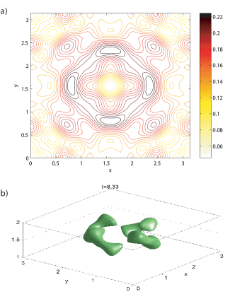
Figure 1: Cut at $z=\frac{\pi}{2}$ of $Q$ (a) and the isosurface $Q(r)=0.8Q_{max}=0.42$ (b).

2.3 Heat diffusion

The simplest quantities to study in order to quantify the evolution of $Q$, are the spatial average $Q(t)=\langle Q(\textbf{r},t)\rangle$ and the root mean square variation $\Delta Q=\sqrt{\langle(Q^{2}-\langle Q\rangle^{2})\rangle}$.

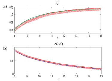
Figure 2: Plots of $Q(t)$ (a) and $\Delta Q(t)/Q(t)$ (b); solid lines are the results of the two-fluid model (see section 3).

These quantities are shown in figure 2, where that the mean heat is seen to increases in time, due to the energy coming from the large eddies, as was shown precedently in [2]. The relative fluctuation $\Delta Q/Q$ is seen to decrease from $0.9$ to $0.2$.

The next natural question is related to the statistical distribution of the small eddies $v^{>}$: are they approximately Gaussian, like an absolute equilibrium? A histogram of $v^{>}_{x}$ is shown in figure 3

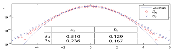
Figure 3: Histogram of $v^{>}_{x}$ and $\tilde{v}^{>}_{x}$ and normalized cumulant $s_{4}$ and $s_{6}$ (odd cumulants vanish because of symmetries).

. As the heat is not homogeneous, we also computed the histogram of the normalized field $\tilde{v}^{>}_{x}=v^{>}_{x}/\sqrt{Q}$ which seems to better obey Gaussian statistics as can be seen on figure 3 and comparing the firsts normalized cumulant $s_{n}=\frac{c_{n}}{\sqrt{c_{2}^{n}}}$ ($c_{n}$ is the cumulant of order $n$) in the table.

3 Two-fluid Model

We now introduce our phenomenological two-fluid model of the truncated Euler equation. One of the fluids describes the large scale velocity field and the other represents the thermalized high-wavenumber modes described by a temperature field $T=Q/c$ ($c$ is the specific heat, explicitly given by $c=8k_{\rm{max}}^{3}$). This model is somewhat analogous to Landau’s standard two-fluid model of liquid Helium at finite temperature $T$ where there is a natural cut-off wavenumber for thermal excitations: the classical-quantum crossover wavenumber $k_{\rm max}$ given by $\hbar k_{\rm max}c_{S}=k_{B}T$ ($c_{S}$ is the sound velocity and $k_{B}$ Boltzmann’s constant). In Landau’s model $k_{\rm max}$ is temperature dependent and the specific heat $c$ is proportional to $T^{3}$. In constrast, $k_{\rm{max}}$ and the specific heat are constant in our model that reads:

$$\partial_{t}v_{i}^{<}+v_{j}^{<}\partial_{j}v_{i}^{<} = -\partial_{i}\tilde{p}+\partial_{j}\sigma^{\prime}_{ij}$$ (7)

$$\partial_{i}v_{i}^{<} = 0$$ (8)

$$\partial_{t}T+v_{j}^{<}\partial_{j}T = \mathcal{D}T+\frac{1}{2c}\left(\partial_{j}v_{i}^{<}+\partial_{i}v_{j}^{<}\right)\sigma^{\prime}_{ij}$$ (9)

where

$$\sigma^{\prime}_{ij} = \mathcal{F}^{-1}[\nu_{\rm{eff}}({k})(ik_{i}\hat{v}_{j}^{<}+ik_{j}\hat{v}_{i}^{<})]$$ (10)

$$\mathcal{D}T = \mathcal{F}^{-1}[-k^{2}D_{\rm{eff}}(k)\mathcal{F}[T]]$$ (11)

and $\mathcal{F}[\cdot]$ denotes the Fourier transform. $\sigma^{\prime}_{ij}$ is a generalized form of the standard viscous strain tensor [8] . The precise form of the anomalous diffusion terms $\nu_{\rm{eff}}$ and $D_{\rm{eff}}$ will be determined below, in sections 3.1 and 3.2.

The advection terms in equation (7) are readily obtained from the Reynolds equations for the filtered velocity by remarking that the diagonal part of the Reynolds stress can, because of incompressibility, be absorbed in the pressure. Equation (10) represents a simple model of the traceless part of the Reynolds tensor [7]. In the same vein, the advection terms in equation (9) are readily obtained together with higher-order moments (see equation (1) of reference [9]). The dissipation and source terms in (9) are thus simple models of the higher-order moments. It is easy to show that in the present model $\langle\frac{1}{2}{\bf v}^{2}+cT\rangle$ is conserved, corresponding to the energy conservation in the truncated Euler equation.

As the fluctuations $\Delta Q/Q$ are small (see above) we will furthermore assume that $\nu_{\rm{eff}}$ and $D_{\rm{eff}}$ only depend on $<Q>=E_{\rm th}$. Thus the evolution of the filtered velocity ${\bf v^{<}}$ is independent of the fluctuations $\Delta Q$. As $[E_{\rm th}]=L^{2}T^{-2}$, simple dimensional analysis yields the following form for the function $\nu_{\rm{eff}}$ and $D_{\rm{eff}}$:

$$\nu_{\rm{eff}}=\frac{\sqrt{E_{\rm{th}}}}{k_{\rm{max}}}f\left(\frac{k}{k_{\rm{max}}},\frac{k_{0}}{k_{\rm{max}}}\right)\,;D_{\rm{eff}}=\frac{\sqrt{E_{\rm{th}}}}{k_{\rm{max}}}\Psi\left(\frac{k}{k_{\rm{max}}},\frac{k_{0}}{k_{\rm{max}}}\right)$$ (12)

where $k_{0}=2\pi/L_{\rm p}$ the smallest nonzero wavenumber ($L_{\rm p}$ is the periodicity length, $2\pi$ in the present simulations).

3.1 EDQNM Determination of viscosity

An analytical determination of function $\nu_{\rm{eff}}$ is possible using the eddy-damped quasi-Markovian theory (EDQNM)[10]. It is known that this model well reproduces the dynamics of truncated Euler Equation, including the $k^{-5/3}$ and $k^{2}$ scalings and the relaxation to equilibrium [11].

The EDQNM closure furnishes an integro-differential equation for the spectrum $E(k,t)$:

$$\frac{\partial E(k,t)}{\partial t}=T_{NL}(k,t)$$ (13)

where the nonlinear transfer $T_{NL}$ is modeled as

$$T_{NL}(k,t) = \int\int\limits_{\triangle}\Theta_{kpq}(xy+z^{3})[k^{2}pE(p,t)E(q,t)$$ (14)

$$- p^{3}E(q,t)E(k,t)]\frac{dp\,dq}{pq}.$$

In (14) $\triangle$ is a strip in $p,q$ space such that the three wavevectors k, p, q form a triangle. $x$, $y$, $z$, are the cosine of the angles opposite to k, p, q. $\Theta_{kpq}$ is a characteristic time defined as

$$\Theta_{kpq}=\frac{1-\exp{(-(\eta_{k}+\eta_{p}+\eta_{q})t)}}{\eta_{k}+\eta_{p}+\eta_{q}}$$ (15)

and the eddy damped $\eta$ is defined as

$$\eta_{k}=\lambda\sqrt{\int\limits_{0}^{k}s^{2}E(s,t)\,ds}.$$ (16)

Classically $\lambda=0.36$ and the truncation is imposed omitting all interactions involving waves numbers larger than $k_{\rm{max}}$ in (14).

A simple and important stationary solution of (13) is the absolute equilibrium with equipartition of the kinetic energy and corresponding spectrum $E(k)\sim k^{2}$.

To compute the EDQNM effective viscosity $\nu_{\rm{eff}}$ we consider an absolute equilibrium with a small perturbation added in the mode of wavenumber $k_{pert}$ and study the relaxation to equilibrium. The corresponding ansatz is $E(p,t)=\frac{3E_{\rm{th}}}{k_{\rm{max}}^{3}}p^{2}+\gamma(t)\delta(p-k_{\rm{pert}})$ and we suppose $E_{\rm{th}}\gg\gamma$, so that the total energy is almost constant and equal to $E_{\rm{th}}$.

Using the long time limit of (15) and expanding the EDQNM transfer (14) to first order in $\gamma$ yields for the delta containing part, after a lengthy but straightforward computation:

$$T_{NL}(k,t)=-\gamma(t)\delta(k-k_{\rm{pert}})k^{2}\frac{\sqrt{E_{\rm{th}}}}{k_{\rm{max}}}\frac{\sqrt{30}}{\lambda}I\left(\frac{k}{k_{\rm{max}}}\right)$$ (17)

where $I$ is given by the explicit integral

$$I(x)=\sqrt{x}\int\limits_{1}^{\frac{2-x}{x}}\int\limits_{-1}^{1}\frac{(p^{2}-1)(1-q^{2})(q^{2}+p^{2}(1+2q^{2})))}{(p^{2}-q^{2})(2^{\frac{5}{2}}+((p-q)^{\frac{5}{2}}+(p+q)^{\frac{5}{2}}))}\,dq\,dp$$

Using (13), (17) and the basic definition of the two-fluid model (7-11), we obtain

$$\nu_{\rm{eff}}(k)=\frac{\sqrt{E_{\rm{th}}}}{k_{\rm{max}}}\frac{\sqrt{30}}{2\lambda}I\left(\frac{k}{k_{\rm{max}}}\right).$$ (18)

The function $f(x=\frac{k}{k_{\rm{max}}},0)$ in (12) is thus given by

$$f(x,0)=\frac{\sqrt{30}}{2\lambda}I(x).$$ (19)

In the limit $x\to 0$, it is simple to show that $f$ has a finite value $f(0,0)=\frac{7}{\sqrt{15}\lambda}$. Thus the EDQNM prediction in the small $k/k_{\rm{max}}$ limit is

$$\nu_{\rm{eff}}=\frac{\sqrt{E_{\rm{th}}}}{k_{\rm{max}}}\frac{7}{\sqrt{15}\lambda},$$ (20)

with $\frac{7}{\sqrt{15}\lambda}=5.021$ for the classic value of $\lambda=0.36$. This asymptotic value can also be obtained from the EDQNM eddy viscosity expression calculated by Lesieur and Schertzer [12] using an energy spectrum $E(k)\sim k^{2}$.

3.2 Monte-Carlo determination of viscosity and thermal diffusion

In order to numerically determine the effective viscosity $\nu_{\rm{eff}}(k)$ of the two-fluid model, we use a general-periodic code to study the relaxation of an absolute equilibrium perturbed by adding a stationary solution of the Euler equation. We thus consider the initial condition

$$u = \cos{kx}\sin{ky}+u_{\rm{eq}}$$ (21)

$$v = -\sin{kx}\cos{ky}+v_{\rm{eq}}$$ (22)

$$w = w_{\rm{eq}}$$ (23)

where the (solenoidal and Gaussian) absolute equilibrium velocity field satisfies $\langle u_{\rm{eq}}^{2}+v_{\rm{eq}}^{2}+w_{\rm{eq}}^{2}\rangle=2E_{\rm{th}}$.

The resulting amplitude of the rotation in (21-23) is found, after a short transient, to decay exponentially in time.

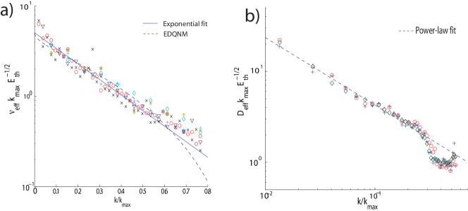
Figure 4: Effective viscosity $\nu_{\rm{eff}}$ (a) and thermal diffusivity $D_{\rm{eff}}$ (b) determined by Monte Carlo computations performed at different values of $E_{\rm th}$ and $k_{\rm{max}}$ (see text).

The function $\nu_{\rm{eff}}(k)$ is then obtained by finding the halving time $\tau_{k}$, for which $\hat{v}_{\alpha}({\bf k},t_{0}+\tau_{k})=\hat{v}_{\alpha}({\bf k},t_{0})/2$, with $t_{0}$ chosen larger than the short transient time. The effective dissipation thus reads

$$\nu_{\rm{eff}}(k)=\log{2}/(k^{2}\tau_{k}).$$ (24)

The values of $\nu_{\rm{eff}}(k)k_{\rm{max}}/\sqrt{E_{\rm{th}}}$ are shown in figure (4a) for different values of $E_{\rm{th}},k,k_{\rm{max}}$. A very good agreement with the EDQNM prediction is observed. Note that there is not dependence in the dimensionless parameter $k_{0}/k_{\rm{max}}$ (see eq. (12)).

An exponential fit of all data in figure 4a gives

$$\nu_{\rm{eff}}=5.0723\frac{\sqrt{E_{\rm th}}}{k_{\rm{max}}}e^{-3.97k/k_{\rm{max}}}.$$ (25)

Note that the limit $k/k_{\rm{max}}\to 0$ is consistent with the EDQNM prediction (20).

Another simple numerical experiment can be used to characterize the thermal diffusion: the relaxation of a spatially-modulated pseudo-equilibrium defined by

$$\left\langle u^{2}+v^{2}+w^{2}\right\rangle=2E_{\rm th}+2\epsilon\cos{(kx)}$$ (26)

with $\epsilon<E_{\rm th}$.

An $x$-dependent temperature can be recovered by averaging $u^{2}+v^{2}+w^{2}$ over $y$ and $z$. Numerical integration of the truncated Euler equation with the initial condition (26) produces an amplitude $\epsilon$ that decays exponentially, as in the case studied for the determination of effective viscosity. The thermal diffusivity $D_{\rm{eff}}$ is determined in the same way as in eq. (24) and the corresponding data is shown in figure 4b. A power-law fit gives

$$D_{\rm{eff}}=0.7723\frac{\sqrt{E_{\rm th}}}{k_{\rm{max}}}(k/k_{\rm{max}})^{-0.74}.$$ (27)

The negative exponent in (27) is characteristic of hypodiffusive processes.

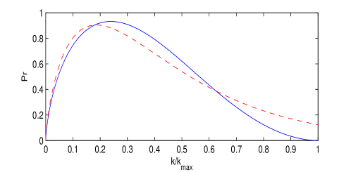
Figure 5: Effective Prandtl number $P_{\rm{eff}}=\nu_{\rm{eff}}/D_{\rm{eff}}$.

We can define an effective Prandtl number as the ratio $P_{\rm{eff}}(k)=\nu_{\rm{eff}}(k)/D_{\rm{eff}}(k)$. The Prandtl number is plotted in figure 5, where the solid blue line is obtained using the EDQNM prediction (20) and the fit (27) and the dashed red line is obtained using the fits (25) and (27). Note that the Prandtl vanishes in the the small $k/k_{\rm{max}}$ limit and verifies $P_{\rm{eff}}<1$ for all wavenumbers.

3.3 Validation of the Model

In this section, numerical integration of the the two-fluid model equations (7-11) are performed using a pseudo-spectral code. Time marching is done using second-order leapfrog finite difference scheme and even and odd time-steps are periodically re-coupled by fourth-order Runge-Kutta. The effective viscosity and diffusivity are updated at each time step by resetting $E_{\rm th}=<Q>$. The obtained data is compared with that directly produced from the truncated Euler equation.

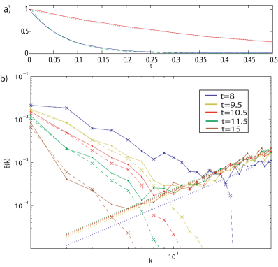
Figure 6: a)Time decay of rotation (21-22) (upper curve) and temperature modulation (26) (bottom curve). Solid line: truncated Euler equations and dashed line: two-fluid model. b)Time-evolution of energy spectra, truncated Euler equation: solid lines and two-fluid model: dashed lines.

The time-evolutions resulting from initial data (21-22) (in red) and (26) (in blue), both normalized to one and with the same value of $E_{\rm{th}}$ is displayed on figure 6a . Good agreement with the two-fluid model is obtained in both cases and the faster relaxation of the temperature modulation is related to the smallness of $P_{\rm{eff}}<1$.

We now compare, the evolution of non-trivial spectra of the truncated Euler equation (1) and the two-fluid model. The truncated Euler equation is integrated using the Taylor-Green initial data. At $t\sim 8$, when a clear scales separation is present, the large-scale fields $\bf{v^{<}}$ (see eq.4) and the heat $Q$ (eq.6) are computed and used as initial data for the two-fluid model (7-11). The subsequent evolution of the two-fluid model is then compared with that of the truncated Euler equation.

Both spectra, plotted in figure 6b, are in good agreement. The straights lines represents the thermalized zone $E(k,t)=c(t)k^{2}$ in the the spectrum of the truncated Euler equation, where $c(t)$ is determined by the condition $\langle Q(t)\rangle=\sum\limits_{k>k_{\rm{th}}}c(t)k^{2}$.

The value of $Q(t)$ and $\Delta Q/Q$ are plotted in figure 2 (solids lines); the evolution of the fluctuation of the temperature are well reproduced too by the two-fluid model.

4 Conclusion

The thermalized small scales were found to follow a quasi-normal distribution. The effective viscosity was determined, using both EDQNM and Monte Carlo. (Hypo)diffusion of heat was obtained and the effective Prandtl number found to vanish at small $k/k_{\rm max}$. The two-fluid model was found to be in good quantitative agreement with the original truncated Euler equations. We acknowledge useful scientific discussions with A. Pouquet and the support of ECOS and CONICYT.

References

- [1] S. Orszag, Statistical Theory of Turbulence, in, Les Houches 1973: Fluid dynamics, R. Balian and J.L. Peube eds. Gordon and Breach, New York, 1977.
- [2] C. Cichowlas, P. Bonaïti, M. Brachet, Effective dissipation and turbulence in spectrally truncated euler flows, Phys. Rev. Lett. 95 (26).
- [3] C. Cichowlas, Equation d’Euler tronquée: de la dynamique des singularités complexes à la relaxation turbulente, Université Pierre et Marie Curie - Paris VI, 2005.
- [4] S. Dyachenko, A. Newell, A. Pushkarev, V. E. Zakharov, Optical turbulence: weak turbulence, condensates and collapsing filaments in the nonlinear Schrödinger equation, Physica D 57 (1992) 96–160.
- [5] C. Connaughton, S. Nazarenko, Warm cascades and anomalous scaling in a diffusion model of turbulence, Phys. Rev. Lett. 92 (4) (2004) 044501.
- [6] G. I. Taylor, A. E. Green, Mechanism of the production of small eddies from large ones, Proc. Roy. Soc. Lond. A 158 (1937) 499–521.
- [7] B. Mohammadi, O. Pironneau, Analysis of the turbulence model, John Wiley & Sons, Masson, 1994.
- [8] L.Landau, E.Lifchitz., Mécanique des Fluides, MIR., 1971.
- [9] B. E. Launder, G. J. Reece, W. Rodi, Progress in the development of a Reynolds-stress turbulence closure, J. Fluid Mech. 68 (1975) 537–566.
- [10] S. Orzag, Analytical theories of turbulence, J. Fluid Mech. 41 (363).
- [11] W. J. T. Bos and J.-P. Bertoglio., Dynamics of spectrally truncated inviscid turbulence, Phys. Fluids 18 (071701).
- [12] M. Lesieur, D. Schertzer, Amortissement auto-similaire d’une turbulence à grand nombre de Reynolds, J. Mec. 17 (1978) 609.