Measuring Fine Tuning In Supersymmetry

Abstract

The solution to fine tuning is one of the principal motivations for supersymmetry. However constraints on the parameter space of the Minimal Supersymmetric Standard Model (MSSM) suggest it may also require fine tuning (although to a much lesser extent). To compare this tuning with different extensions of the Standard Model (including other supersymmetric models) it is essential that we have a reliable, quantitative measure of tuning. We review the measures of tuning used in the literature and propose an alternative measure. We apply this measure to several toy models and the MSSM with some intriguing results.

1 Introduction

The Little Hierarchy Problem arose when no Beyond the Standard Model (BSM) physics was found at LEP, despite expectations from naturalness that it would. In particular Barbieri and Giudice Barbieri:1987fn argued that to avoid fine tuning the supersymmetric particles of the Constrained Minimal Supersymmetric Standard Model (CMSSM) should be within the mass reach of LEP.

The mass of the $Z$ boson is predicted from the soft supersymmetry (susy) breaking parameters by imposing electroweak symmetry breaking conditions. For $\tan{\beta}=10$,

$\frac{M_{Z}^{2}}{2}\approx-|\mu|^{2}+0.076m_{0}^{2}+1.97m_{\frac{1}{2}}^{2}+0.1A^{2}+0.38Am_{\frac{1}{2}}$, where the parameters are $m_{0}$, the universal scalar mass; $m_{1/2}$, the universal gaugino mass; $A$, the universal trilinear coefficient; ${\rm sign}(\mu)$, the undetermined sign of $\mu$, a bilinear soft Higgs mass, and $\tan\beta$. Although the correct $M_{Z}=91.1876$ GeV can be obtained by fixing $|\mu|$, if $1.97m_{1/2}\approx 500$ then this must cancel with some combination of parameters to ${\cal O}(1/25)$.

To quantify tuning Barbieri and Guidice applied a measure originally proposed in Ref.Ellis:1986yg . For an observable, $O$, and a parameter, $p_{i}$, $\triangle_{BG}(p_{i})=\Big{|}\frac{p_{i}}{O(p_{i})}\frac{\partial O(p_{i})}{\partial p_{i}}\Big{|}\rm{.}$

A large value of $\triangle_{BG}(p_{i})$ implies that a small change in the parameter results in a large change in the observable, so the parameters must be carefully “tuned” to the observed value. Since there is one $\triangle_{BG}(p_{i})$ per parameter, they define the largest of these values to be the tuning for that scenario, $\triangle_{BG}=\rm{max}(\{\triangle_{BG}(p_{i})\})\rm{.}$ They then make the aesthetic choice that $\triangle_{BG}>10$ is fine tuned.

Despite wide use of $\triangle_{BG}$, it has several limitations which may obscure the true picture of tuning:

• variations in each parameter are considered separately;

• only one observable is considered in the tuning measure, but there may be tunings in several observables;

• only infinitesimal variations in the parameters are considered;

• there is an implicit assumption that the parameters come from uniform probability distributions.

• it does not take account of global sensitivity;

The final problem can be understood by considering the simple mapping $f:x\rightarrow x^{n}$, where $n\gg 1$. For this function $\triangle_{BG}=\triangle_{BG}(x)=n$. Since $\triangle_{BG}$ is independent of $x$, we follow the example of Anderson:1994dz and term this global sensitivity. Since $\triangle_{BG}(x_{1})-\triangle_{BG}(x_{2})=0$ for all $x_{1},x_{2}$, there is no relative sensitivity between points in the parameter space.

If we use $\triangle_{BG}$ as our tuning measure then $f(x)$ appears fine tuned throughout the entire parameter space. This contrasts with our fundamental notion of tuning being a measure of how atypical a scenario is. A true measure of tuning should only be greater than one when there is relative sensitivity between different points in the parameter space.

2 A New Tuning Measure

We propose a new measure of tuning. We define two volumes in parameter space for every point $P^{\prime}\{p_{i}^{\prime}\}$. $F$ is the volume formed from dimensionless variations in the parameters over some arbitrary range $[a,b]$, about point $P^{\prime}$, i.e. $a\leq\frac{p_{i}}{p_{i}^{\prime}}\leq b$. $G$ is the volume in which dimensionless variations of the observables fall into the same range $[a,b]$, i.e. $a\leq\frac{O_{j}(\{p_{i}\})}{O_{j}(\{p_{i}^{\prime}\})}\leq b$.

We define an unnormalised measure of tuning with, $\triangle=\frac{F}{G}\rm{.}$ This can be used to compare different regions of parameter space within a given model as the normalisation factor will be common. However like $\triangle_{BG}$ it includes global sensitivity. To compare tuning in different models we need to include normalisation, so tuning is given by,

$$\triangle=\frac{F}{G}\rm{,}\,\,\,\,\;\;\;\;\hat{\triangle}=\frac{1}{\bar{\triangle}}\frac{F}{G}\rm{,}$$ (1)

$$\rm{with},\,\bar{\triangle}=\left\langle\frac{F}{G}\right\rangle=\frac{\int dp_{1}...dp_{n}\frac{F}{G}(\{p_{i}\},\{O_{i}\})}{\int dp_{1}...dp_{n}}\rm{.}$$ (2)

It is also useful to look at tuning in terms of individual observables, while maintaning our multi-parameter approach. Therefore we define $G_{O_{j}}$ to be the volume restricted by $a\leq\frac{O_{j}(\{p_{i}\})}{O_{j}(\{p_{i}^{\prime}\})}\leq b$ and $a\leq\frac{p_{i}}{p_{i}^{\prime}}\leq b$. Tuning is then defined by,

$$\hat{\triangle}_{O_{j}}=\frac{1}{\left\langle\frac{F}{G_{O_{j}}}\right\rangle}\frac{F}{G_{O_{j}}}\rm{,}$$ (3)

2.1 Probabilistic Interpretation

$G$ is a volume containing physical scenarios which are “similar” to point P, where our notion of similarity is given by $a$, $b$. Assuming every point in parameter space is equally likely, the probability of a randomly selected point lying in $G$ is $G/V_{T}$, where $V_{T}$ is some hypothesised total volume of parameter space. If there existed some volume, $T$, which was “typical” in size, the probability of a random point lying in it would be $T/V_{T}$. Our expectation for the volume $G$ is based on the magnitude of the parameters. The volume formed by “similar” parameters is a way of combing the magnitudes of each parameter into one one volume which describes them all. This is our volume $F$. Knowing only the volume of $F$ we can find the $G$ we would typically expect by comparing it to the average ratio between $F$ and $G$. So for parameters “similar” in size to those at point P, the volume one typically expects “similar” physical scenarios to form is $T=F/\bar{\triangle}$. Therefore we can associate our new measure of tuning with relative improbability, $\hat{\triangle}\sim\frac{P(T)}{P(G)}$.

3 Applications

As a first example we determine the tuning for a toy version of the Standard Model (SM) Hierarchy Problem with only one observable, the physical Higgs (mass)², $m_{H}^{2}$, and one parameter, $m_{0}^{2}$. At one loop we write, $m^{2}_{H}=m^{2}_{0}-C\Lambda^{2}$, where $\Lambda$, the Ultra-Violet cutoff, is taken to be the Planck Mass, while $C$ is a positive constant.

Variations in $m_{0}^{2}$ give a line of length $F=(b-a)m_{0}^{2}$, while variations in the observable, $m_{H}^{2}$, give another line, of length $G=(b-a)m_{H}^{2}$.

$$\Rightarrow\triangle=m_{0}^{2}/m_{h}^{2}=\triangle_{BG}\approx 10^{34}$$ (4)

The arbitrary range $[a,b]$ has fallen out of the result.

We also determine $\bar{\triangle}$, by integrating over the whole parameter range, $m^{2}_{0\,min}<m_{0}^{2}<m_{0\,max}^{2}$ where $m^{2}_{0\,max}$, $m^{2}_{0\,min}$ are hypothetical upper and lower limits respectively and present results where $m_{H}^{2}>0$. These bounds give the total allowed range of the parameter in this model and should not be confused with the range of dimensionless variations which appears in the definition of $F$. If we take the range of variation to be large, $m_{0max}^{2}-m_{0min}^{2}\gg C\Lambda^{2}$, then $\hat{\triangle}\approx\frac{m_{0}^{2}}{m_{H}^{2}}=\triangle_{BG}$. Alternatively, if we choose a very narrow range of variation about $C\Lambda^{2}+\mu_{H}^{2}$, where $\mu_{H}\approx 100\,\rm{GeV}$, then $\hat{\triangle}$ is very small.

This is intuitively reasonable. If there was some compelling theoretical reason for the bare mass to be constrained close to the cutoff, the case for new physics at low energies would be dramatically weakened. It is precisely because there is no such compelling reason that we worry about the hierarchy problem and look to low energy BSM physics to explain how we can have $m_{H}\ll M_{\rm Planck}$.

Now lets treat the SM Hierarchy Problem in a slightly more sophisticated way . We no longer fix the UV cutoff. Instead we treat $m_{H}^{2}$ as a function of two parameters, $m_{0}^{2}$ and $\Lambda^{2}$ and we have a second observable $M^{2}_{\rm Planck}=\Lambda^{2}$ (“observed” to be large due to the weakness of gravitation).

There are no new cancellations between the parameters, so we expect the same result for $\triangle$ as before, but this provides a simple illustration of how our measure works with more than one parameter. Varying the parameters about some point $P^{\prime}(m_{0}^{2},\Lambda^{2})$ over the dimensionless interval $[a,b]$ forms an area, $F$. The bounds from dimensionless variations in $m_{H}^{2}$ introduce two new lines in the parameter space which together with dimensionless variations in $M_{\rm Planck}^{2}$ (the same as those from $\Lambda^{2}$), form the area $G$.

This is shown schematically in Fig. 1 for two different points. In one, the parameters are of the same order as the observables (since $M_{\rm Planck}$ is O($m_{H}$)), so $G$ is not much smaller than $F$. For the other point $M^{2}_{\rm Planck}\gg m_{H}^{2}$, resulting in $F\gg G$ and fine tuning. In general the areas are, $F=(b-a)^{2}m_{0}^{2}\Lambda^{2}$ and $G=(b-a)^{2}\Lambda^{2}m_{H}^{2}$ so again we obtain, $\triangle=1+\frac{C\Lambda^{2}}{m_{H}^{2}}=\triangle_{BG}$.

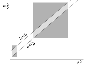
Figure 1: The two dimensional volumes (areas) $F$ (entire grey rectangle) and $G$ (light grey) for two different points in the two dimensional parameter space.

While our measure does not deviate from $\triangle_{BG}$ in this simple example, models with additional parameters allow the observable to be obtained from cancellation of more than two terms, complicating the fine tuning picture. For more examples including one with three parameters and four observables please see Ref. Athron:2007ry .

3.1 Fine Tuning In the CMSSM

Since the CMSSM contains many parameters and many observables we chose to apply a numerical version of our measure to study the variation of tuning in the CMSSM.

We take random dimensionless fluctuations about a CMSSM point at the GUT scale, $P^{\prime}=\{p_{k}\}$, to give new points $\{P_{i}\}$. These are passed to a modified version of Softsusy 2.0.5Allanach:2001kg . Each random point $P_{i}$ is run down from the GUT scale until electroweak symmetry is broken. An iterative procedure is used to predict $M_{Z}^{2}$ and then all the sparticle and Higgs masses are determined.

For every observable $O_{i}$ a count, $N_{O_{i}}$, is kept of how often the point lies in the volume $G_{O_{i}}$ as well as an overall count, $N_{O}$, kept of how many points are in $G$. The tunings are then measured with,

$$\triangle_{O_{i}}\approx\frac{N}{N_{O_{i}}}{\rm,}\,\,\,\triangle\approx\frac{N}{N_{O}}.$$ (5)

The set of observables, $\{O_{j}\}$ used in our definition of $G$ here is the set of $M_{Z}^{2}$ and all (masses)² predicted in Softsusy.

The parameters we vary simultaneously are the set $\{m_{0},m_{1/2},\mu_{GUT},m_{3}^{2},A,y_{t},y_{b},y_{\tau}\}$, where $m_{3}$ is the soft bilinear Higgs mixing parameter and $y_{t},y_{b},y_{\tau}$ are the Yukawa couplings of the top, bottom and tau respectively

When using Softsusy to predict the masses for the random points, sometimes the full mass spectrum cannot be predicted as we may have a tachyon, the Higgs potential unbounded from below, or non-perturbativity. Such points don’t belong in $G$ as they will give dramatically different physics. However it is unclear which volumes, $G_{O_{i}}$, the point lies in. Such points never register as hits in any of the $G_{O_{i}}$ and this may artificially inflate the individual tunings, including $\triangle_{M_{Z}^{2}}$. Keeping the range small reduces such errors, so we chose $a=0.9$ and $b=1.1$ for our dimensionless variations.

We examine tuning for points in the grid,

$$A=-100\,{\rm GeV},\;\;\;\;\tan{\beta}=10,\;\;\;{\rm sign}(\mu)=+,$$

$$250\,{\rm GeV}\leq m_{\frac{1}{2}}\leq 500\,{\rm GeV}{\rm,}\;100\,{\rm GeV}\leq m_{0}\leq 200\,{\rm GeV}.$$

Shown in Fig.2 is the variation in $\triangle_{M_{Z}^{2}}$ with respect to $m_{1/2}$. To reduce statistical errors the $\triangle_{M_{Z}^{2}}$ for each $m_{1/2}$ is averaged over the five different $m_{0}$ values. This substantially reduces the errors giving a much more stable picture of tuning increasing linearly with $m_{1/2}$.

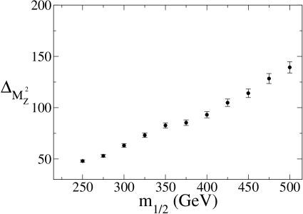
Figure 2: Tuning variation in $M_{Z}^{2}$ plotted against $m_{1/2}$. To reduce statistical errors, at each value of $m_{1/2}$, we have taken the mean value $\triangle_{M_{Z}^{2}}$ over the five different $m_{0}$ values.

$\triangle$, which includes all of the masses predicted by Softsusy as well as $M_{Z}^{2}$, is shown in Fig. 3. Although the errors are much larger here, a similar pattern to that for $M_{Z}^{2}$ can be seen. Since these are unnormalised tunings, the numerical values of the two measures cannot be compared and one should not assume that $\triangle>\triangle_{M_{Z}^{2}}$ implies that the tuning is worse than when only $M_{Z}^{2}$ was considered. In fact the lack of evidence for distinct patterns of variation in tuning from the Figs. 2 and 3 is consistent with the conjecture that the large cancellation between parameters in $M_{Z}^{2}$ is the dominant source of the tuning for these points.

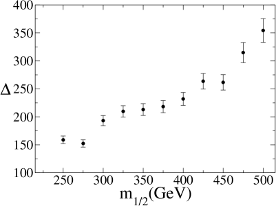
Figure 3: Variation in $\triangle$ plotted as in Fig. 2 for $\triangle_{M_{Z}^{2}}$.

Although we can’t easily determine the normalisation using this approach it is nonetheless interesting to compare the unnormalised tunings for the points in our study with those obtained for points with more “natural” looking spectra. We present two points for this purpose. NP1 and NP2 are defined by,

$\{m_{\frac{1}{2}}=M_{Z}{\rm,}\,\,m_{0}=M_{Z},\,\,A=-M_{Z},\,\,{\rm sign}(\mu)=+,\\ \tan\beta=3\}$ and $\{m_{\frac{1}{2}}=-50\,\rm{GeV}{\rm,}\,\,m_{0}=100\,\rm{GeV},\\ A=-50\,\rm{GeV},\,\,{\rm sign}(\mu)=+,\tan\beta=10\}$ respectively.

The spectra of these points are displayed in Fig. 4 and Fig. 5, and the unnormalised tunings are displayed in Table 1. Note that these are not intended to be “realistic” scenarios. Indeed both NP1 and NP2 are ruled out by experiment but are simply intended to provide “natural” scenarios for comparison.

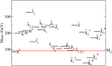
Figure 4: Point NP1 with a “natural” spectrum

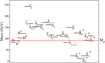
Figure 5: Point NP2 with a “natural” spectrum

	$\triangle$	$\triangle_{M_{Z}^{2}}$	$\triangle_{m_{\chi_{1}^{0}}^{2}}$
NP1	$241^{+36}_{-26}$	$14.7^{+0.5}_{-0.5}$	$30.1^{+1.4}_{-1.3}$
NP2	$31.4^{+1.5}_{-1.4}$	$2.92^{+0.04}_{-0.04}$	$2.64^{+0.04}_{-0.04}$

Table 1: Unnormalised tunings for the two points, NP1 and NP2, with natural looking spectra.

While in NP1 $\triangle_{M_{Z}^{2}}$ is reduced there’s a relatively large tuning in the mass of the lightest neutralino ($\triangle_{m_{\chi_{1}^{0}}^{2}}$). These combine to give a $\triangle$ which is similar in size to the values found for our grid of points. In NP2 all of the tunings are relatively small, but the combined tuning is still larger than may naively have been anticipated. This is because many of these small tunings for individual observables, restricting different regions of parameter space. Table 2 shows the approximate relative magnitude of the tunings in our grid points with respect to these seemingly natural points.

	$\hat{\triangle}$	$\hat{\triangle}_{M_{Z}^{2}}$	$\hat{\triangle}_{m_{\chi_{1}^{0}}^{2}}$
Relative to NP1	$0.5-1.5$	$3-10$	$0.2$
Relative to NP2	$5-15$	$10-50$	$2$

Table 2: Approximate relative tunings for the points in our study, with respect to those for NP1 and NP2.

Notice that if for either NP1 or NP2 we truely had $\triangle^{NP}\approx\bar{\triangle}$ and $\triangle_{M_{Z}}^{NP}\approx\bar{\triangle}_{M_{Z}}$ then we would have demonstrated that $\hat{\triangle}_{M_{Z}}>\hat{\triangle}$ and could conclude that the Little Hierarchy problem is not as severe as has been suggested.

Sometimes (e.g. NP1) the lightest neutralino is very light due to large cancellations between the parameters. Similar effects may be present in other masses, so mass hierarchies may appear in a greater proportion of the parameter space than conventional CMSSM wisdom dictates. This would reduce the true tuning in the CMSSM as scenarios with hierarchies would be less atypical than previously thought. A reduction in tuning from this effect can only be measured by using our normalised new measure, $\hat{\triangle}$.

4 Conclusions

Current measures of tuning have several limitations. They neglect the many parameter nature of fine tuning; ignore additional tunings in other observables; consider local stability only; assume ${\cal L}_{SUSY}$ is parametrised in the same way as ${\cal L}_{GUT}$ and do not account for global sensitivity.

We have presented a new measure of tuning to address these issues. We showed that in the CMSSM both $\triangle$ and $\triangle_{BG}$ increase with $M_{1/2}$. While a naive interpretation suggests $\triangle_{BG}>\triangle$ normalisation may dramatically change this. If $\hat{\triangle}<<\hat{\triangle}_{M_{Z}}$ we can explain the Little Hierarchy Problem.

References

- (1) R. Barbieri and G. F. Giudice, Nucl. Phys. B 306, 63 (1988).
- (2) J. R. Ellis, K. Enqvist, D. V. Nanopoulos and F. Zwirner, Mod. Phys. Lett. A 1 (1986) 57.
- (3) G. W. Anderson and D. J. Castano, Phys. Lett. B 347, 300 (1995) [arXiv:hep-ph/9409419].
- (4) B. C. Allanach, Comput. Phys. Commun. 143, 305 (2002) [arXiv:hep-ph/0104145].
- (5) P. Athron and D. J. Miller, arXiv:0705.2241 [hep-ph].