Search for rare b-meson decays at CDF

Abstract

We report on the search for $B^{0}_{s}\rightarrow\mu^{+}\mu^{-}$, $B^{0}_{d}\rightarrow\mu^{+}\mu^{-}$ decays and $b\rightarrow s\mu^{+}\mu^{-}$ transitions in exclusive decays of B mesons using the CDF II detector at the Fermilab Tevatron Collider. Using 2 fb^-1 of Run II data we find upper limits on the branching fractions $\mathcal{B}(B^{0}_{s}\rightarrow\mu^{+}\mu^{-})<5.8\times 10^{-8}$ and $\mathcal{B}(B^{0}_{d}\rightarrow\mu^{+}\mu^{-})<1.8\times 10^{-8}$ at 95$\%$ confidence level. The results for the branching fractions of the $b\rightarrow s\mu^{+}\mu^{-}$ transitions using 924 pb^-1 of Run II data are $\mathcal{B}(B^{+}\rightarrow\mu^{+}\mu^{-}K^{+})=(0.60\pm 0.15\pm 0.04)\times 10^{-6}$, $\mathcal{B}(B^{0}_{d}\rightarrow\mu^{+}\mu^{-}K^{*0})=(0.82\pm 0.31\pm 0.10)\times 10^{-6}$ and $\mathcal{B}(B^{0}_{s}\rightarrow\mu^{+}\mu^{-}\phi)/\mathcal{B}(B^{0}_{s}\rightarrow J/\psi\phi)<2.61\times 10^{-3}$ at 95$\%$ confidence level.

1 Introduction

The decay of a $b$ quark into two muons, as well as in an $s$ quark and two muons, requires a flavor-changing neutral current (FCNC) process which is highly suppressed in the standard model (SM) as they can only occur through higher order diagrams. New physics can significantly enhance the branching fractions of these decays. In these proceedings the current results of the CDF experiment are presented for the branching ratios of the rare decays $B^{0}_{(s,d)}\rightarrow\mu^{+}\mu^{-}$ and $B\rightarrow\mu^{+}\mu^{-}h$, where $B$ stands for $B^{+}$, $B^{0}_{d}$, or $B_{s}$, and h stands for $K^{+}$,$K^{*0}$ or $\phi$. The $K^{*0}$ is reconstructed in the mode $K^{*0}\rightarrow K^{+}\pi^{-}$ and the $\phi$ is reconstructed as $\phi\rightarrow K^{+}K^{-}$. A detailed description of the analyses can be found in Ref. RefJ2 ; RefJ1 .

2 The CDF II Detector

The CDF II detector is a cylindrical general-purpose particle detector built at one of the two collision points of the Tevatron $p\bar{p}$ collider which operates at a center-of-mass energy of $\sqrt{s}=1.96$ TeV. Its inner tracking system consists of a silicon microstrip detector surrounded by an open-cell wire drift chamber. The tracking systems are immersed in a 1.4 T magnetic field and measure the momentum of charged particles. The electromagnetic and hadronic sampling calorimeters are located outside the solenoid. The outermost part of the CDF II detector is the muon detector system. Muons are detected by the planar drift chambers (CMU) and the central muon extension (CMX), which consists of conical sections of drift tubes. The CMU covers a pseudorapidity range up to $|\eta|<0.6$, where $\eta=-\ln(\tan{\frac{\theta}{2}})$ and $\theta$ is the angle of the track with respect to the beamline, selecting muons with a $p_{T}>1.4$ GeV/c. The CMX extends the coverage to a pseudorapidity range of $0.6<|\eta|<1.0$ for muons with $p_{T}>2.0$ GeV/c.

3 Search Methodology

The searches for the rare decays $B^{0}_{(s,d)}\rightarrow\mu^{+}\mu^{-}$ and $B\rightarrow\mu^{+}\mu^{-}h$ use in both cases a similar approach. A data sample with an integrated luminosity of 2 fb^-1 is used for $B^{0}_{(s,d)}\rightarrow\mu^{+}\mu^{-}$ search, respectively 924 pb^-1 for the $B\rightarrow\mu^{+}\mu^{-}h$ search. In both cases events are selected by the dimuon trigger. For the $B^{0}_{(s,d)}\rightarrow\mu^{+}\mu^{-}$ analysis the data is futher divided into two classes. Either both muons are reconstructed in the CMU chambers, further called CMU-CMU, or one muon is reconstructed in the CMX chambers and the other in the CMU chambers, called CMU-CMX.

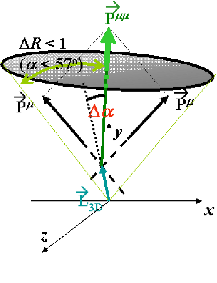
Figure 1: Graphical representation of the discriminating variables.

3.1 Selection Optimization

To optimize the data selection a signal event sample from MC simulation and a background sample from data sidebands is used.
In case of the $B^{0}_{(s,d)}\rightarrow\mu^{+}\mu^{-}$ analysis a multivariate neural network (NN) enhances the signal and background separation. It is based on the discriminating variables illustrated in Figure 1: the proper decay length $\lambda=\beta\gamma c\tau$, the 3D opening angle $\Delta\theta$ between the dimuon momentum $\vec{p}^{\mu\mu}$ and the displacement vector from the primary to the dimuon vertex $\vec{L}$, the $p_{T}$ of the lower momentum muon candidate and the B-candidate isolation $I$ ISO .
In case of the $B\rightarrow\mu^{+}\mu^{-}h$ analysis a cut based approach is used to optimize the selection for the figure of merit $S/\sqrt{S+B}$, where $S$ is the estimate of the expected yield of the rare decays and $B$ is the expected background. The discriminating variables are the decay length significance $\lambda/\sigma_{\lambda}$, the pointing angle $\alpha$ from the B meson candidate to the primary vertex and the isolation $I$. For the final selection candidates with a dimuon mass near the $J/\psi$ and the $\psi^{\prime}$ are rejected.

3.2 Normalization Modes

In order to obtain the branching ratios of the different rare decays, one normalizes to the $B\rightarrow J/\psi h$ modes. The branching ratios for the decays $B\rightarrow\mu^{+}\mu^{-}h$ are then given by

$$\frac{\mathcal{B}(B\rightarrow\mu^{+}\mu^{-}h)}{\mathcal{B}(B\rightarrow J/\psi h)} = \frac{N_{\mu^{+}\mu^{-}h}}{N_{J/\psi h}}\frac{\epsilon_{J/\psi h}}{\epsilon_{\mu^{+}\mu^{-}h}}\cdot\mathcal{B}(J/\psi\rightarrow\mu^{+}\mu^{-})$$

where $N_{\mu^{+}\mu^{-}h}$ is the observed number of $B\rightarrow\mu^{+}\mu^{-}h$ decays, $N_{J/\psi h}$ is the observed number of $B\rightarrow J/\psi h$ decays, while $\epsilon_{J/\psi h}$ and $\epsilon_{\mu^{+}\mu^{-}h}$ are the selection efficiencies of $B\rightarrow J/\psi h$ and $B\rightarrow\mu^{+}\mu^{-}h$ respectively. The ratio of efficiencies is about 70 to 85 % RefJ2 .
In case of the rare decays $B^{0}_{(s,d)}\rightarrow\mu^{+}\mu^{-}$ the upper limit on the branching fraction can be expressed as

$$\mathcal{B}(B^{0}_{s,d}\rightarrow\mu^{+}\mu^{-})^{95\%\mbox{\tiny C.L.}} = \frac{N^{95\%}_{B^{0}_{s,d}}}{N_{B^{+}}}\cdot\frac{\alpha_{B^{+}}}{\alpha_{B^{0}_{s,d}}}\cdot\frac{\epsilon^{\mbox{\tiny base}}_{B^{+}}}{\epsilon^{\mbox{\tiny base}}_{B^{0}_{s,d}}}\cdot\frac{1}{\epsilon^{\mbox{\tiny NN}}_{B^{0}_{s,d}}}$$

$$\cdot\frac{f_{u}}{f_{s,d}}\cdot\mathcal{B}(B^{+}\rightarrow J/\psi K^{+})$$

where $N^{95\%}_{B^{0}_{s,d}}$ is the upper limit on the number of $B^{0}_{s,d}\rightarrow\mu^{+}\mu^{-}$ decays at the 95$\%$ C.L. determined from the comparison between expected and observed background events, $N_{B^{+}}$ is the number of reconstructed $B^{+}\rightarrow J/\psi K^{+}$ candidates. The parameters $\alpha$, $\epsilon^{\mbox{\tiny base}}$ and $\epsilon^{\mbox{\tiny{NN}}}$ are the trigger acceptances and the efficiencies of the initial, respectively the NN, requirements. $\frac{f_{u}}{f_{s,d}}$ denotes the ratio between the probabilities that a $b$ quark produced in a ppbar collisions hadronizes into a $B^{+}$ meson and a $B_{s}$ or $B_{d}$ meson RefJ1 .

3.3 Background Estimation

To estimate the background contributions several different sources are considered.
In case of the rare decays $B\rightarrow\mu^{+}\mu^{-}h$ these sources are charmless B decays into charged hadrons, reflections between the three rare decay modes and combinatorial background. The background originating from charmless B decays is calculated from a simulation of these decays convoluted with the misidentification rates of muon detectors obtained from $D^{*}$-tagged $D^{0}\rightarrow K^{-}\pi^{+}$ decays. The combinatorial background is estimated from the high mass sidebands of the $B$ signal and extrapolated under the signal region using the background shape from the data distribution with poor vertex quality.
In case of the $B^{0}_{s,d}\rightarrow\mu^{+}\mu^{-}$ decays the background consists of contributions from $B^{0}_{s,d}\rightarrow h^{+}h^{-}$, where $h^{\pm}=\pi^{\pm}$ or $K^{\pm}$, and combinatoric background. The expected background from $B^{0}_{s,d}\rightarrow h^{+}h^{-}$ is calculated from equation 3.2 by replacing $B^{0}_{s,d}\rightarrow\mu^{+}\mu^{-}$ with $B^{0}_{s,d}\rightarrow h^{+}h^{-}$ and including two additional efficiency terms to account for the muon misidentification rates, measured in $D^{0}\rightarrow K\pi$ data, and the fraction of misidentified $B^{0}_{s,d}\rightarrow h^{+}h^{-}$ events falling in the signal windows. The branching ratio for the various $B^{0}_{s,d}\rightarrow h^{+}h^{-}$ modes are taken from Ref. RefJ3 . The combinatoric background is estimated by extrapolating the number of events in the sideband regions passing a given cut to the signal region using a linear fit. The total background is then formed by summing up the combinatoric background and the contributions from $B^{0}_{s,d}\rightarrow h^{+}h^{-}$ decays.

4 Results

4.1 $B\rightarrow\mu^{+}\mu^{-}h$

In case of the rare decays $B\rightarrow\mu^{+}\mu^{-}h$ we observe an excess in the signal region in all three decay modes. The invariant mass distributions are shown in Figures 1, 1 and 1. The significance of the excess is determined by calculating the probability for the background to fluctuate into the number of observed events. The results for the number of observed events, expected background events, the significance and the absolute and relative branching ratios are listed in table 1. The branching ratios are calculated using equation 3.2. We find

$$\frac{\mathcal{B}(B^{+}\rightarrow\mu^{+}\mu^{-}K^{+})}{\mathcal{B}(B^{+}\rightarrow J/\psi K^{+})} = (0.59\pm 0.15\pm 0.03)\times 10^{-3}$$

$$\frac{\mathcal{B}(B^{0}_{d}\rightarrow\mu^{+}\mu^{-}K^{*0})}{\mathcal{B}(B^{0}_{d}\rightarrow J/\psi K^{*0})} = (0.62\pm 0.23\pm 0.07)\times 10^{-3}$$

$$\frac{\mathcal{B}(B^{0}_{s}\rightarrow\mu^{+}\mu^{-}\phi)}{\mathcal{B}(B^{0}_{s}\rightarrow J/\psi\phi)} = (1.24\pm 0.60\pm 0.15)\times 10^{-3}$$

Using the world average branching ratios of the normalization modes Yao , we find

$$\mathcal{B}(B^{+}\rightarrow\mu^{+}\mu^{-}K^{+}) = (0.60\pm 0.15\pm 0.04)\times 10^{-6}$$

$$\mathcal{B}(B^{0}_{d}\rightarrow\mu^{+}\mu^{-}K^{*0}) = (0.82\pm 0.31\pm 0.10)\times 10^{-6}$$

$$\mathcal{B}(B^{0}_{s}\rightarrow\mu^{+}\mu^{-}\phi) = (1.16\pm 0.56\pm 0.42)\times 10^{-6}$$

Since the excess in $B^{0}_{s}\rightarrow\mu^{+}\mu^{-}\phi$ is not significant, we calculate a limit on its relative branching ratio using Bayesian integration assuming a flat prior, and find at $95(90)\%$ C.L.

$$\frac{\mathcal{B}(B^{0}_{s}\rightarrow\mu^{+}\mu^{-}\phi)}{\mathcal{B}(B^{0}_{s}\rightarrow J/\psi\phi)} < 2.61(2.30)\times 10^{-3}$$

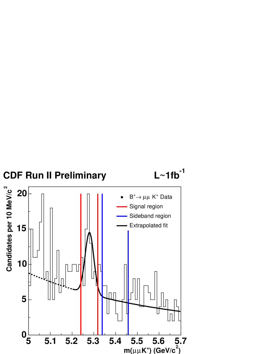
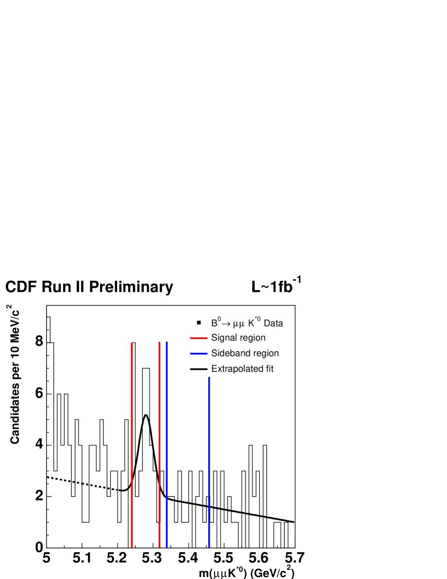
Figure 2: Inv. mass spectrum for the decay $B^{+}\rightarrow\mu^{+}\mu^{-}K^{+}$.

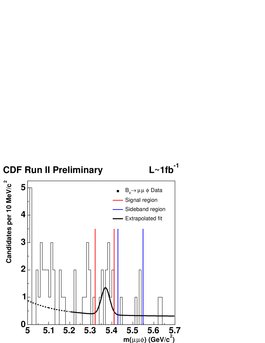
Figure 3: Inv. mass spectrum for the decay $B^{0}_{d}\rightarrow\mu^{+}\mu^{-}K^{*0}$.

Figure 4: Inv. mass spectrum for the decay $B^{0}_{s}\rightarrow\mu^{+}\mu^{-}\phi$.

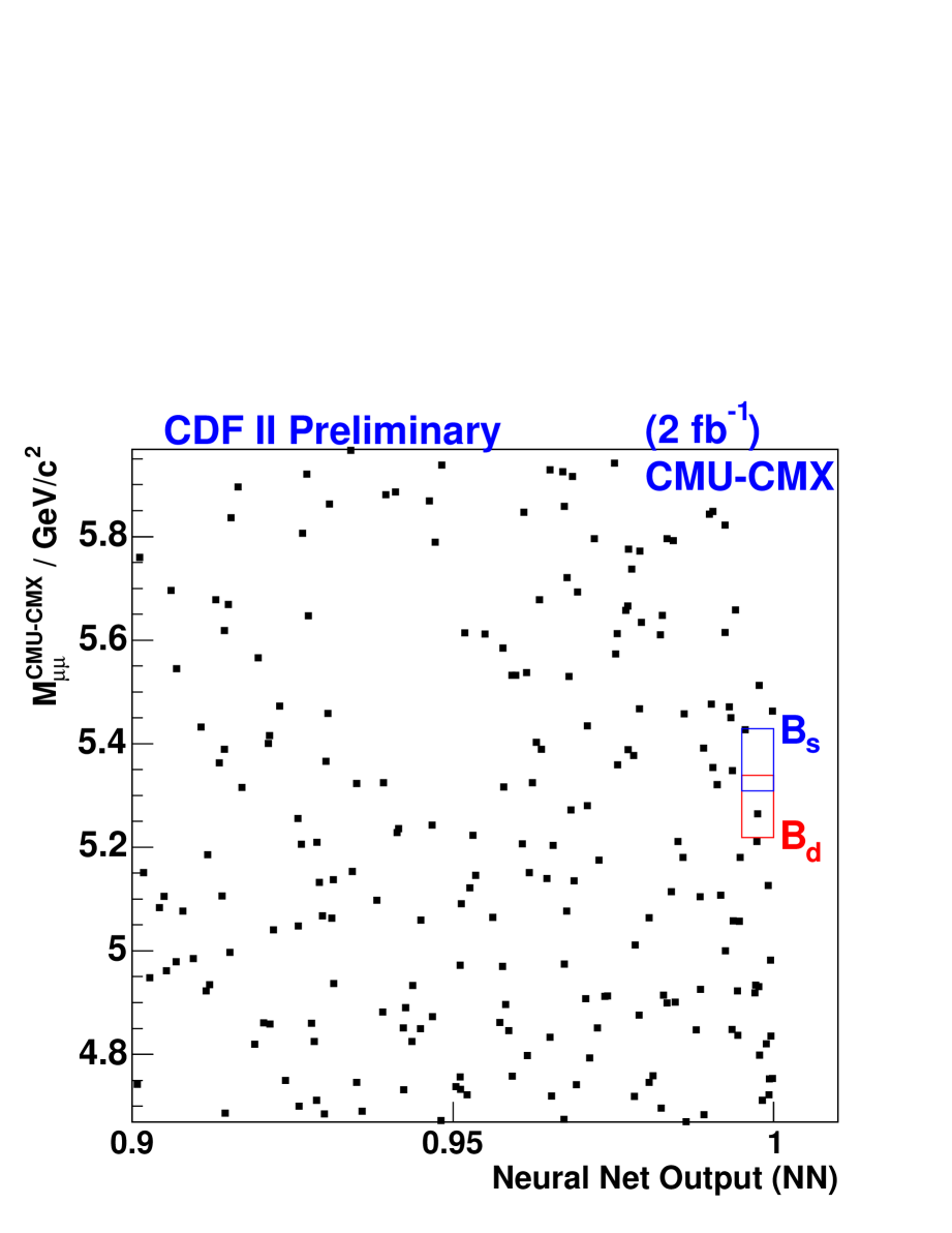
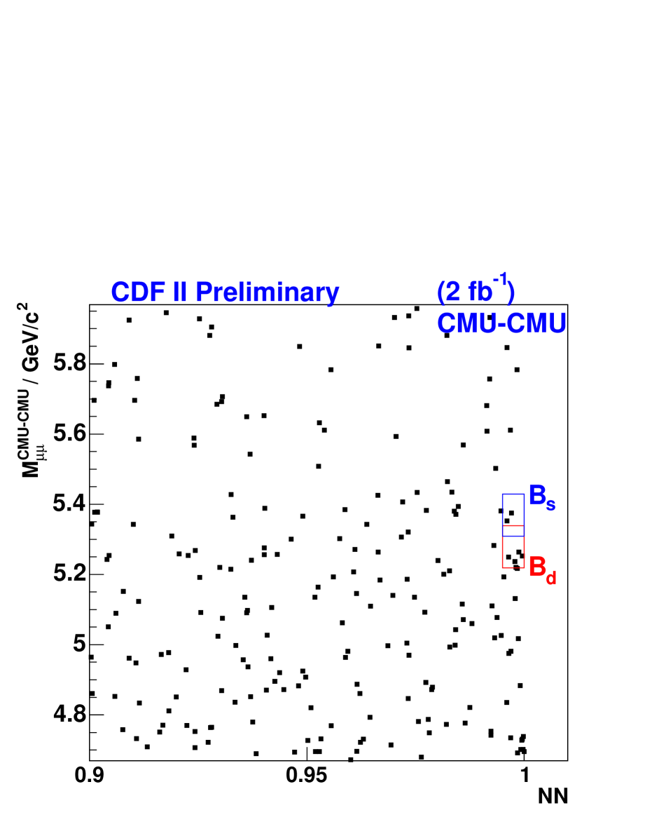
Figure 5: The invariant mass distribution versus the NN output for the CMU-CMX channel.

Figure 6: The invariant mass distribution versus the NN output for the CMU-CMU channel.

4.2 $B^{0}_{s,d}\rightarrow\mu^{+}\mu^{-}$

In case of the rare decays $B^{0}_{s,d}\rightarrow\mu^{+}\mu^{-}$ we use different neural network bins and mass bins for the computation of the limits on the branching ratios. Table 2 shows the number of expected and observed events of the two trigger scenarios CMU-CMU and CMU-CMX for different cuts on the network output NN and gives the result on the branching ratio for the combination of both scenarios with a neural network cut of $NN>0.80$. In Figures 6 and 6 the invariant mass distribution vs. the neural network value is displayed. Using equation 3.2 we obtain the $90(95)\%$ C.L. limits

$$\mathcal{B}(B^{0}_{s}\rightarrow\mu^{+}\mu^{-})<4.7\times 10^{-8}(5.8\times 10^{-8})$$

$$\mathcal{B}(B^{0}_{d}\rightarrow\mu^{+}\mu^{-})<1.5\times 10^{-8}(1.8\times 10^{-8})$$

5 Conclusion

We present the latest results on the measurement of the branching ratios of the rare decays $B\rightarrow\mu^{+}\mu^{-}h$ and give an upper limit on the branching ratio of the decays $B^{0}_{s,d}\rightarrow\mu^{+}\mu^{-}$. The results for the branching ratios for the decay modes $B^{+}\rightarrow\mu^{+}\mu^{-}K^{+}$ and $B^{0}\rightarrow\mu^{+}\mu^{-}K^{*0}$ are in good agreement with the results of the B factory experiments BABAR and BELLE BABAR ; BELLE . The limit on the branching fraction $\mathcal{B}(B^{0}_{s}\rightarrow\mu^{+}\mu^{-}\phi)$/
$\mathcal{B}(B^{0}_{s}\rightarrow J/\psi\phi)$ is the most stringent to date. The new results for the upper limit for the branching ratio of the decays $B^{0}_{s,d}\rightarrow\mu^{+}\mu^{-}$ are currently the world’s best limits and can be used to reduce the allowed parameter space of a broad spectrum of SUSY models SUSY01 ; SUSY02 ; SUSY03 ; SUSY04 .

Table 1: Results of the $B\rightarrow\mu^{+}\mu^{-}h$ analysis.

Mode	$B^{+}\rightarrow\mu^{+}\mu^{-}K^{+}$	$B^{0}_{d}\rightarrow\mu^{+}\mu^{-}K^{*0}$	$B^{0}_{s}\rightarrow\mu^{+}\mu^{-}\phi$
$N_{S}$	$90$	$35$	$11$
$N_{BG}$	$45.3\pm 5.8$	$16.5\pm 3.6$	$3.5\pm 1.5$
Gaussian significance $(\sigma)$	$4.5$	$2.9$	$2.4$
Rel $\mathcal{B}\pm stat\pm sys\times 10^{-3}$	$0.59\pm 0.15\pm 0.03$	$0.62\pm 0.23\pm 0.07$	$1.24\pm 0.60\pm 0.15$
Abs $\mathcal{B}\pm stat\pm sys\times 10^{-6}$	$0.60\pm 0.15\pm 0.04$	$0.82\pm 0.31\pm 0.10$	$1.16\pm 0.56\pm 0.42$
Rel $\mathcal{B}$ 95% CL limit $\times 10^{-3}$	-	-	$2.61$
Rel $\mathcal{B}$ 90% CL limit $\times 10^{-3}$	-	-	$2.30$

Table 2: Expected number of background (exp.) and number of observed (obs.) events in the CMU-CMU and CMU-CMX channels for the $B^{0}_{s}$ mass window (5.310-5.430 GeV/c²) and the $B^{0}_{d}$ mass window (5.219-5.339 GeV/c²).

	Mode	$B^{0}_{d}\rightarrow\mu^{+}\mu^{-}$	$B^{0}_{s}\rightarrow\mu^{+}\mu^{-}$
CMU-CMU	N exp., $0.800<$NN$<0.950$	$25.5\pm 0.7$	$23.5\pm 0.7$
CMU-CMU	N obs., $0.800<$NN$<0.950$	32	18
CMU-CMU	N exp., $0.950<$NN$<0.995$	$8.5\pm 0.5$	$7.7\pm 0.5$
CMU-CMU	N obs., $0.950<$NN$<0.995$	7	10
CMU-CMU	N exp., $0.995<$NN	$2.4\pm 0.2$	$2.1\pm 0.2$
CMU-CMU	N obs., $0.995<$NN	5	2
CMU-CMX	N exp., $0.800<$NN$<0.950$	$27.8\pm 0.9$	$26\pm 0.7$
CMU-CMX	N obs., $0.800<$NN$<0.950$	28	26
CMU-CMX	N exp., $0.950<$NN$<0.995$	$10.8\pm 0.5$	$10.3\pm 0.5$
CMU-CMX	N obs., $0.950<$NN$<0.995$	6	11
CMU-CMX	N exp., $0.995<$NN	$1.6\pm 0.2$	$1.6\pm 0.2$
CMU-CMX	N obs., $0.995<$NN	1	1
combined	Abs $\mathcal{B}$ 95% CL limit $\times 10^{-8}$	$1.8$	$5.8$
combined	Abs $\mathcal{B}$ 90% CL limit $\times 10^{-8}$	$1.5$	$4.7$

6 Acknowledgments

The author would like to thank the members of the CDF Collaboration who performed the analyses.

References

- (1) CDF Collaboration, CDF Public Note 8543, (2006)
- (2) CDF Collaboration, CDF Public Note 8956, (2007)
- (3) A. Abulencia et al., Phys. Rev. Lett. 97, 211802 (2006)
- (4) W.M. Yao et al., J. Phys. G 33, 1 (2006)
- (5) R. Dermisek et al., J. High Energy Phys. 09, 029 (2005)
- (6) R. Ruiz de Austri et al., J. High Energy Phys. 0605, 002 (2006)
- (7) S. Baek et al., J. High Energy Phys. 0506, 017 (2005)
- (8) R. Arnowitt et al., Phys. Lett B 538, 121 (2002)
- (9) B. Aubert et al. [BABAR Collaboration], Phys. Rev. D 73, 092001 (2006), arXiv:hep-ex/0604007
- (10) K. Abe et al. [BELLE Collaboration], arXiv:hep-ex/0410006
- (11) The B-candidate isolation is defined as , where the sum is over all tracks with ; and are the azimuthal angle and pseudorapidity of track with respect to .