Graphical Representation of SUSY and Application to QFT

Abstract

We present a graphical representation of the supersymmetry and the graphical calculation. Calculation is demonstrated for 4D Wess-Zumino model and for Super QED. The chiral operators are graphically expressed in an illuminating way. The tedious part of SUSY calculation, due to manipulating chiral suffixes, reduces considerably. The application is diverse.

The supersymmetry is the symmetry between fermions and bosons. It was introduced in the mid 70’s. At present the experiment does not yet confirm the symmetry, but everybody accepts its importance in nature and expects fruitful results in the future developement. The requirement of such a high symmetry costs a sophisticated structure which makes its dynamical analysis difficult. In this circumstance, we propose a calculational technique which utilizes the graphical representation of SUSY. The representation was proposed in SI03 ; SUSY2004 . The spinor is represented as a slanted line with a direction. Its chirality is represented by the way the line is drawn. The advantage of the graph expression is the use of the graph indices. Every independent graph, which corresponds to a unique term in the ordinary calculation, is classified by a set of graph indices. Hence the main efforts of programinng is devoted to find good graph indices and to count them. SUSY calculation generally is not a simple algebraic or combinatoric or analytical one. It involves the vast branch of mathematics including Grassmann algebra. The delicate property of chirality is produced in this environment. It requires a basic language for flexible programming. We take C-language and present the output of a first-step program.

Weyl spinors have the SU(2)${}_{L}\times$SU(2)_R structure. The chiral suffix $\alpha$, appearing in $\psi^{\alpha}$ or $\psi_{\alpha}$, represents (fundamental representation, doublet representation) SU(2)_L and the anti-chiral suffix ${\dot{\alpha}}$, appearing in ${\bar{\psi}}^{\dot{\alpha}}$ or ${\bar{\psi}}_{\dot{\alpha}}$, represents SU(2)_R. The raising and lowering of suffixes are done by the antisymmetric tensors $\epsilon^{\alpha\beta}$ and $\epsilon_{\alpha\beta}$.

$$(\epsilon^{\alpha\beta})=\left(\begin{array}[]{cc}0&1\\ -1&0\end{array}\right),\ (\epsilon_{{\dot{\alpha}}{\dot{\beta}}})=\left(\begin{array}[]{cc}0&-1\\ 1&0\end{array}\right),\ \epsilon^{\alpha\beta}\epsilon_{\beta\gamma}=\delta^{\alpha}_{\gamma},$$ (5)

$$\psi^{\alpha}=\epsilon^{\alpha\beta}\psi_{\beta},\ {\bar{\psi}}_{\dot{\alpha}}=\epsilon_{{\dot{\alpha}}{\dot{\beta}}}{\bar{\psi}}^{\dot{\beta}}.$$ (6)

They are graphically expressed by Fig.1.

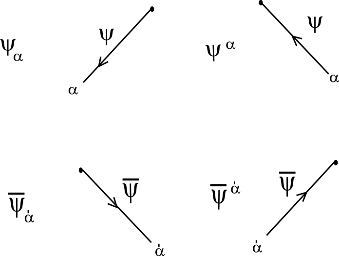
Figure 1: Weyl fermions.

We encode them as follows. We use 2 dimensional array with the size 2$\times$2. The four chiral spinors are stored in C-program as the array psi[ ][ ].

(1) (Weyl) Spinor [Symbol: p ; Dimension: M^3/2 ]
$\psi^{\alpha}$ psi[0,0]=$\alpha$ psi[0,1]=emp psi[1,0]=emp psi[1,1]=emp   $\psi_{\alpha}$ psi[0,0]=emp psi[0,1]=$\alpha$ psi[1,0]=emp psi[1,1]=emp   ${\bar{\psi}}_{\dot{\alpha}}$ psi[0,0]=emp psi[0,1]=emp psi[1,0]=emp psi[1,1]=${\dot{\alpha}}$   ${\bar{\psi}}^{\dot{\alpha}}$ psi[0,0]=emp psi[0,1]=emp psi[1,0]=${\dot{\alpha}}$ psi[1,1]=emp

The first column takes two numbers 0 and 1; 0 expresses a ’chiral’ operator $\psi$, while 1 expresses an ’anti-chiral’ operator ${\bar{\psi}}$. The second column also takes the two numbers; 0 expresses an ’up’ suffix, while 1 expresses an ’down’ one.

Note: ’emp’ means ’empty’ and is expressed by a default number (, for example, 99) in the program.

(2) Sigma Matrix [Symbol: s ; Dimension: M⁰ ]
 Sigma matrices $\sigma^{m},{\bar{\sigma}}^{m}$ are graphically expressed in Fig.2.

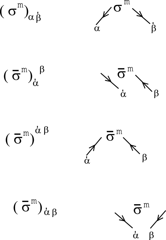
Figure 2: Elements of SL(2,C) $\sigma$-matrices. $(\sigma^{m})_{\alpha{\dot{\beta}}}$ and $({\bar{\sigma}}^{m})^{{\dot{\alpha}}\beta}$ are the standard form.

They are stored as the 2$\times$2 array si[ ][ ].
$\sigma^{m}_{~{}\alpha{\dot{\alpha}}}$ si[0,0]=emp si[0,1]=$\alpha$ si[1,0]=emp si[1,1]=${\dot{\alpha}}$ siv=m   ${\bar{\sigma}}^{m{\dot{\alpha}}\alpha}$ si[0,0]=${\dot{\alpha}}$ si[0,1]=emp si[1,0]=$\alpha$ si[1,1]=emp siv=m

(3)Superspace coordinate[Symbol: t; Dimension: M^-1/2 ]
The superspace coordinate $\theta^{\alpha}$ is exprssed in the same way as the spinor $\psi^{\alpha}$.

$\theta^{\alpha}$ th[0,0]=$\alpha$ th[0,1]=emp th[1,0]=emp th[1,1]=emp   $\theta_{\alpha}$ th[0,0]=emp th[0,1]=$\alpha$ th[1,0]=emp th[1,1]=emp   ${\bar{\theta}}_{\dot{\alpha}}$ th[0,0]=emp th[0,1]=emp th[1,0]=emp th[1,1]=${\dot{\alpha}}$   ${\bar{\theta}}^{\dot{\alpha}}$ th[0,0]=emp th[0,1]=emp th[1,0]=${\dot{\alpha}}$ th[1,1]=emp
They are graphically expressed by Fig.3.

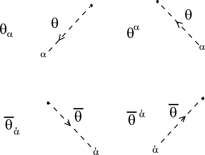
Figure 3: The graphical representation for the spinor coordinates in the superspace: $\theta_{\alpha},\theta^{\alpha},{\bar{\theta}}_{\dot{\alpha}}$ and ${\bar{\theta}}^{\dot{\alpha}}$.

(4) Gagino [Symbol: l ; Dimension: M^3/2 ]
The photino $\lambda^{\alpha}$ is exprssed in the same way as the spinor $\psi^{\alpha}$. We take the 2$\times$2 array la[ ][ ].

$\lambda^{\alpha}$ la[0,0]=$\alpha$ la[0,1]=emp la[1,0]=emp la[1,1]=emp   $\lambda_{\alpha}$ la[0,0]=emp la[0,1]=$\alpha$ la[1,0]=emp la[1,1]=emp   ${\bar{\lambda}}_{\dot{\alpha}}$ la[0,0]=emp la[0,1]=emp la[1,0]=emp la[1,1]=${\dot{\alpha}}$   ${\bar{\lambda}}^{\dot{\alpha}}$ la[0,0]=emp la[0,1]=emp la[1,0]=${\dot{\alpha}}$ la[1,1]=emp

In the process of SUSY calculation, there appear graphs connected by directed lines (chiral suffixes contraction) and by (non-directed) dotted lines (vector suffixes contraction). We can classify them by some graph indices: (1)vpairno The number of vector-suffix contractions; (2)NcpairO The number of chiral-suffix contractions. This is equal to the number of left-directed wedges; (3)NcpairE The number of anti-chiral-suffix contractions. This is equal to the number of the right-directed wedges; (4)closed-chiral-loop-No The closed-chiral-loop is the case that the directed lines , connected by $\sigma$ or ${\bar{\sigma}}$, make a loop. In this case NcpairO=NcpairE. The number of closed chiral loops is defined to this index; (5)GrNum A group is defined to be a set of $\sigma$’s or ${\bar{\sigma}}$’s which are connected by directed lines. The number of groups is defined to be GrNum.

In TABLE 1-2, we list the classification of the product of $\sigma$’s using the graph indices defined above.

vpairno	NcpairO	NcpairE	figure
	0	0	$\begin{array}[]{c}\mbox{ \leavevmode\resizebox{30.35216pt}{}{\includegraphics*{sig2Ar.eps} } }\end{array}$
0	0	1	$\begin{array}[]{c}\mbox{ \leavevmode\resizebox{30.35216pt}{}{\includegraphics*{sig2Cr.eps} } }\end{array}$
	1	0	$\begin{array}[]{c}\mbox{ \leavevmode\resizebox{30.35216pt}{}{\includegraphics*{sig2Cbr.eps} } }\end{array}$
	1	1	$\begin{array}[]{c}\mbox{ \leavevmode\resizebox{30.35216pt}{}{\includegraphics*{sig2Dr.eps} } }\end{array}\ =-2\eta^{mn}$
	0	0	$\begin{array}[]{c}\mbox{ \leavevmode\resizebox{30.35216pt}{}{\includegraphics*{sig2Br.eps} } }\end{array}\ =-2\epsilon_{\alpha\beta}\epsilon_{{\dot{\alpha}}{\dot{\beta}}}$
1	0	1	$\begin{array}[]{c}\mbox{ \leavevmode\resizebox{30.35216pt}{}{\includegraphics*{sig2Fr.eps} } }\end{array}\ =-4\delta^{\beta}_{\alpha}$
	1	0	$\begin{array}[]{c}\mbox{ \leavevmode\resizebox{30.35216pt}{}{\includegraphics*{sig2Fbr.eps} } }\end{array}\ =-4\delta_{\dot{\beta}}^{\dot{\alpha}}$
	1	1	$\begin{array}[]{c}\mbox{ \leavevmode\resizebox{30.35216pt}{}{\includegraphics*{sig2Er.eps} } }\end{array}\ =-8$
TABLE 1 Classification of the product of 2 sigma matrices.

vpairno	NcpairO	NcpairE	figure
	0	0	$\begin{array}[]{c}\mbox{ \leavevmode\resizebox{30.35216pt}{}{\includegraphics*{sig3Ar.eps} } }\end{array}$
0	0	1	$\begin{array}[]{c}\mbox{ \leavevmode\resizebox{30.35216pt}{}{\includegraphics*{sig3Cbr.eps} } }\end{array}$
	1	0	$\begin{array}[]{c}\mbox{ \leavevmode\resizebox{30.35216pt}{}{\includegraphics*{sig3Cr.eps} } }\end{array}$
	1	1	closed-chiral-loop No =1 $\begin{array}[]{c}\mbox{ \leavevmode\resizebox{30.35216pt}{}{\includegraphics*{sig3Er.eps} } }\end{array}$
			closed-chiral-loop No =0 $\begin{array}[]{c}\mbox{ \leavevmode\resizebox{30.35216pt}{}{\includegraphics*{sig3Gr.eps} } }\end{array}$
	0	0	$-2\epsilon_{\alpha\beta}\epsilon_{{\dot{\alpha}}{\dot{\beta}}}\ \begin{array}[]{c}\mbox{ \leavevmode\resizebox{30.35216pt}{}{\includegraphics*{sig3Br.eps} } }\end{array}$
1	0	1	$-4\delta^{\beta}_{\alpha}\ \begin{array}[]{c}\mbox{ \leavevmode\resizebox{30.35216pt}{}{\includegraphics*{sig3Dr.eps} } }\end{array}$
	1	0	$-4\delta^{\dot{\alpha}}_{\dot{\beta}}\ \begin{array}[]{c}\mbox{ \leavevmode\resizebox{30.35216pt}{}{\includegraphics*{sig3Dr.eps} } }\end{array}$
	1	1	$-8\ \begin{array}[]{c}\mbox{ \leavevmode\resizebox{30.35216pt}{}{\includegraphics*{sig3Fr.eps} } }\end{array}$
TABLE 2 Classification of the product of 3 sigma matrices.

These tables clearly show the $\sigma$-matrices play an important role to connect the chiral world and the space-time (Lorentz) world.

Supersymmetry is most manifestly expressed in the superspace $(x^{m},\theta,{\bar{\theta}})$. $\theta_{\alpha}=\epsilon_{\alpha\beta}\theta^{\beta}$, ${\bar{\theta}}^{\dot{\alpha}}=\epsilon^{{\dot{\alpha}}{\dot{\beta}}}{\bar{\theta}}_{\dot{\beta}}$ are spinorial coordinates. They satisfy the relations graphically shown in Fig.4.

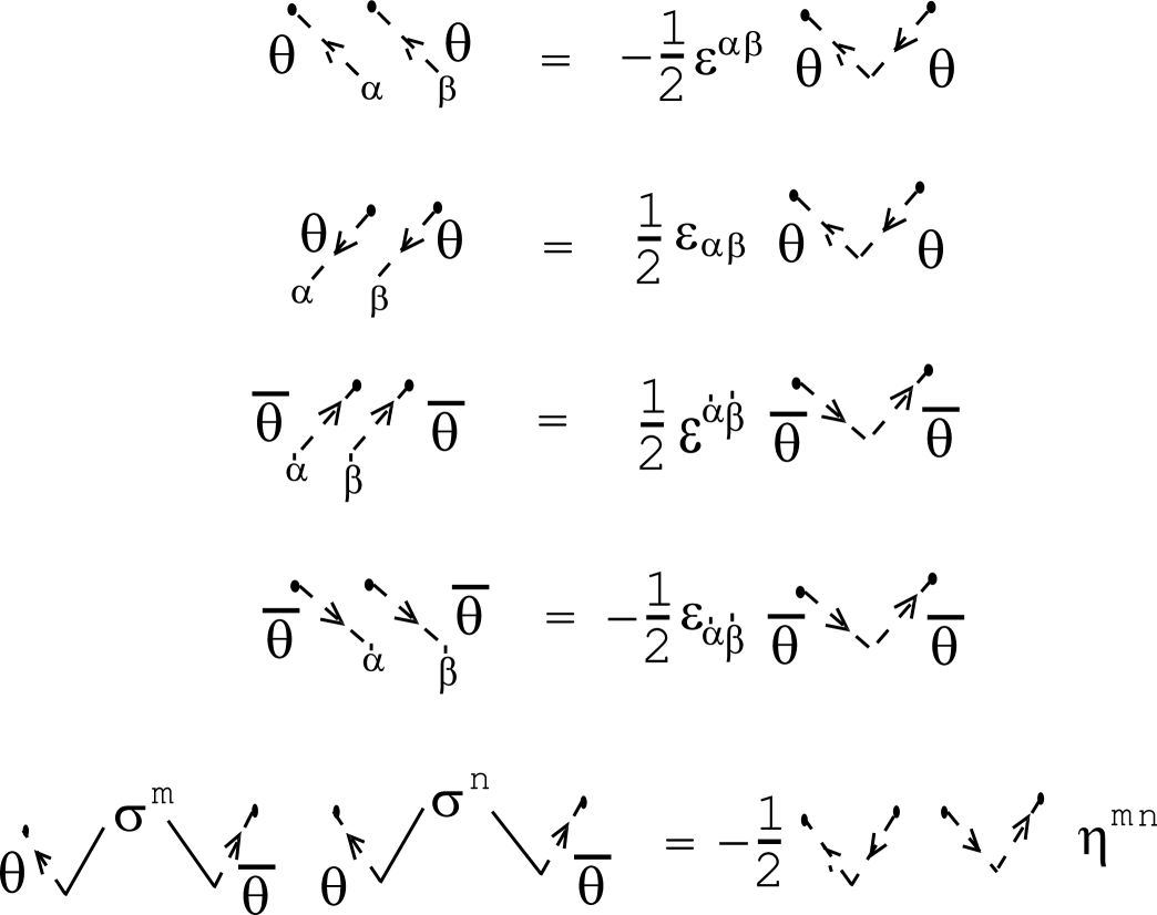
Figure 4: The graphical rules for the spinor coordinates: $\theta^{\alpha}\theta^{\beta}=-{\frac{1}{2}}\epsilon^{\alpha\beta}\theta\theta,~{}\theta_{\alpha}\theta_{\beta}={\frac{1}{2}}\epsilon_{\alpha\beta}\theta\theta,~{}{\bar{\theta}}^{\dot{\alpha}}{\bar{\theta}}^{\dot{\beta}}={\frac{1}{2}}\epsilon^{{\dot{\alpha}}{\dot{\beta}}}{\bar{\theta}}{\bar{\theta}},~{}{\bar{\theta}}_{\dot{\alpha}}{\bar{\theta}}_{\dot{\beta}}=-{\frac{1}{2}}\epsilon_{{\dot{\alpha}}{\dot{\beta}}}{\bar{\theta}}{\bar{\theta}},~{}\theta\sigma^{m}{\bar{\theta}}\theta\sigma^{n}{\bar{\theta}}=-{\frac{1}{2}}\theta\theta{\bar{\theta}}{\bar{\theta}}\eta^{mn}$.

These relations are exploited in the program in order to sort the SUSY quantities with respect to the power of $\theta\theta$ and ${\bar{\theta}}{\bar{\theta}}$.

For the totally anti-symmetric tensor $\epsilon^{lmns}$, we introduce one dimensional array ep[ ] with 4 components.

    ep[0]=l ep[1]=m ep[2]=n ep[3]=s     Symbol:  e    

This term appears later and produces topologically important terms such as $v_{lm}{\tilde{v}}^{lm}=\epsilon^{lmns}v_{lm}v_{ns}$.

As for the metric of the chiral suffix, we do not introduce specific arrays. They play a role of raising or lowering suffixes, which can be encoded in the upper (0) and lower (1) code in arrays. For the Lorentz metric $\eta^{mn}$, we do not need to much care for the discrimination between the upper and lower suffixes because of the even-symmetry with respect to the change of the Lorentz suffixes($\eta^{mn}=\eta^{nm}$).

The ”reduction” formulae (from the cubic $\sigma^{\prime}$s to the linear one) are expressed as in Fig.5.

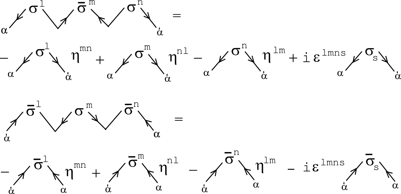
Figure 5: Two relations: 1) $\sigma^{l}{\bar{\sigma}}^{m}\sigma^{n}=-\sigma^{l}\eta^{mn}+\sigma^{m}\eta^{nl}-\sigma^{n}\eta^{lm}+i\epsilon^{lmns}\sigma_{s}$, 2) ${\bar{\sigma}}^{l}\sigma^{m}{\bar{\sigma}}^{n}=-{\bar{\sigma}}^{l}\eta^{mn}+{\bar{\sigma}}^{m}\eta^{nl}-{\bar{\sigma}}^{n}\eta^{lm}-i\epsilon^{lmns}{\bar{\sigma}}_{s}$.

From Fig.5, we notice any chain of $\sigma^{\prime}$s can always be expressed by less than three $\sigma^{\prime}$s. The appearance of the 4th rank anti-symmetric tensor $\epsilon^{lmns}$ is quite illuminating. The following closed chiral-loop graph reduces to an interesting quantity.

$$\begin{array}[]{c}\mbox{ \leavevmode\resizebox{50.59209pt}{}{\includegraphics*{ssbssbBR.eps} } }\end{array}=2(\eta^{lm}\eta^{ns}-\eta^{ln}\eta^{ms}+\eta^{ls}\eta^{mn}$$ (8)

$$-i\epsilon^{lmns})$$ (9)

The transformation between the superfield expression and the fields-components expression is an important subject of SUSY theories. For the purpose, we do the calculation of $\Phi^{\dagger}\Phi$. In this case, the input data is taken from the content of the superfield.

$$\Phi^{\dagger}=-i\begin{array}[]{c}\mbox{ \leavevmode\resizebox{30.35216pt}{}{\includegraphics*{PHI1r.eps} } }\end{array}\partial_{m}A^{*}+\begin{array}[]{c}\mbox{ \leavevmode\resizebox{30.35216pt}{}{\includegraphics*{PHI2r.eps} } }\end{array}\frac{1}{4}\partial^{2}A^{*}$$ (12)

$$+2\begin{array}[]{c}\mbox{ \leavevmode\resizebox{30.35216pt}{}{\includegraphics*{PHIB3r.eps} } }\end{array}+i\begin{array}[]{c}\mbox{ \leavevmode\resizebox{30.35216pt}{}{\includegraphics*{PHIB4r.eps} } }\end{array}+\begin{array}[]{c}\mbox{ \leavevmode\resizebox{30.35216pt}{}{\includegraphics*{PHIB5r.eps} } }\end{array}F^{*}+A^{*}$$ (16)

where the directed dotted line is the superspace coordinate $\theta^{\alpha}$. This data of $\Phi^{\dagger}$ is stored as

weight[sf=0,t=0]=0+i(-1) type[sf=0,t=0,c=0]= t th[sf=0,t=0,c=0,0,0]=1 type[sf=0,t=0,c=1]= s si[sf=0,t=0,c=1,0,1]=1 si[sf=0,t=0,c=1,1,1]=2 siv[sf=0,t=0,c=1]=51 type[sf=0,t=0,c=2]= t th[sf=0,t=0,c=2,1,0]=2 type[sf=0,t=0,c=3]= B B[sf=0,t=0,c=3,1]=51 weight[sf=0,t=1]=1+i(0) type[sf=0,t=1,c=0]= t th[sf=0,t=1,c=0,0,0]=1 type[sf=0,t=1,c=1]= t th[sf=0,t=1,c=1,0,1]=1 type[sf=0,t=1,c=2]= t th[sf=0,t=1,c=2,1,1]=2 type[sf=0,t=1,c=3]= t th[sf=0,t=1,c=3,1,0]=2 type[sf=0,t=1,c=4]= C C[sf=0,t=1,c=4,1]=1

$\cdot\cdot\cdot$

The calculation of $\Phi{\dagger}\Phi$ leads to the Wess-Zumino Lagrangian.

$$\Phi^{\dagger}\Phi|_{\theta^{2}{\bar{\theta}}^{2}}=-{\frac{1}{2}}\partial_{m}A^{*}\partial^{m}A\ +\frac{1}{4}\partial^{2}A^{*}\cdot A\ +\frac{1}{4}A^{*}\partial^{2}A$$

$$-i\times(-1)\begin{array}[]{c}\mbox{ \leavevmode\resizebox{30.35216pt}{}{\includegraphics*{OutFig2r.eps} } }\end{array}\ +i\times(-1)\begin{array}[]{c}\mbox{ \leavevmode\resizebox{30.35216pt}{}{\includegraphics*{OutFig1r.eps} } }\end{array}\ +F^{*}F$$ (19)

We donot ignore the total divergence here.

We also do the calculation of $W_{\alpha}W^{\alpha}$ where $W_{\alpha}$ is the field strength superfield. They are expressed as follows.

$$W_{\alpha}=-i\begin{array}[]{c}\mbox{ \leavevmode\resizebox{15.17607pt}{}{\includegraphics*{WalD1r.eps} } }\end{array}+\begin{array}[]{c}\mbox{ \leavevmode\resizebox{15.17607pt}{}{\includegraphics*{WalD2r.eps} } }\end{array}D$$ (22)

$$-i\begin{array}[]{c}\mbox{ \leavevmode\resizebox{50.59209pt}{}{\includegraphics*{WalD3r.eps} } }\end{array}{\frac{1}{2}}v_{mn}+\begin{array}[]{c}\mbox{ \leavevmode\resizebox{50.59209pt}{}{\includegraphics*{WalD4r.eps} } }\end{array}$$ (25)

This data of $W_{\alpha}$ is stored as

weight[sf=0,t=0]=0+i(-1) type[sf=0,t=0,c=0]= l la[sf=0,t=0,c=0,0,1]=1 weight[sf=0,t=1]=1+i(0) type[sf=0,t=1,c=0]= t th[sf=0,t=1,c=0,0,1]=1 type[sf=0,t=1,c=1]= D D[sf=0,t=1,c=1]=1

$\cdot\cdot\cdot$

The kinetic term of the photon and the photino, in the SuperQED, is given by

$${\cal L}=\frac{1}{4}(-W_{\alpha}W^{\alpha}|_{\theta^{2}}+{\bar{W}}_{\dot{\alpha}}{\bar{W}}^{\dot{\alpha}}|_{{\bar{\theta}}^{2}})$$

$$=-\frac{1}{4}{v_{mn}}^{2}+\frac{i}{2}(\begin{array}[]{c}\mbox{ \leavevmode\resizebox{30.35216pt}{}{\includegraphics*{OutFig2r.eps} } }\end{array}-\begin{array}[]{c}\mbox{ \leavevmode\resizebox{30.35216pt}{}{\includegraphics*{OutFig1r.eps} } }\end{array})+{\frac{1}{2}}D^{2}\ ,$$ (28)

where we do not ignore the total divergence.

In the history of the quantum field theory, new techniques have produced physically important results. The regularization techniques are such examples. The dimensional regularization by ’tHooft and VeltmanTV72 produced important results on the renormalization group property of Yang-Mills theory and many scattering amplitude calculations. The lattice regularization in the gauge theory revealed non-perturbative features of hadron physics. In this case, the computor technique of numerical calculation is essential. As for the computer algebraic one, we recall the calculation of 2-loop on-shell counterterms of pure Einstein gravityGS85 ; Ven92 . A new technique is equally important as a new idea.

The SUSY theory is beautifully constructed respecting the symmetry between bosons and fermions, but the attractiveness is practically much reduced by its complicated structure: many fields, chiral properties, Grassmannian algebra, etc. The present approach intends to improve the situation by a computer program which makes use of the graphical technique. (This approach is taken in Ref.SI98IJMPC for the calculation of product of SO(N) tensors. It was applied to various anomaly calculations. )

The present program should be much more improved. Here we cite the prospective final goal.

1. It can do the transformation between the superfield expression and the component expression.

2. It can do the SUSY trnasformation of various quantities. In particular it can confirm the SUSY-invariance of the Lagrangian in the graphical way and give the final total divergence.

3. It can do algebraic SUSY calculation involving $D_{\alpha},{\bar{D}}^{\dot{\alpha}},Q_{\alpha}$ and ${\bar{Q}}^{\dot{\alpha}}$.

The item 1 above has been demostrated in the present paper for the simple cases of Wess-Zumino model and the Super QED.

It is impossible to deal with all SUSY calculations. This is simply because which fields appear and which dimensional quantities are calculated depend on each problem. If we obatin a list of (graph) indices which classify all physical quantities (operators) appearing in the output, then the present program works (by adding new lines for the new problem).

References

• (1) S. Ichinose, hep-th/0301166, DAMTP-2003-8, US-03-01, ”Graphical Representation of Supersymmetry”
• (2) S. Ichinose, hep-th/0410027, Proc. 12th Int.Conf. on ”Supersymmetry and Unification of Fundamental Interactions”(June 17-23,2004,Epochal Tsukuba Congress Center,Japan), p853-856, ”Graphical Representation of Supersymmetry and Computer Calculation”
• (3) S. Ichinose, hep-th/0603214, Univ. Vienna preprint UWThPh-2006-7, ”Graphical Representation of Supersymmetry”
• (4) S. Ichinose, hep-th/0603220, Univ. Vienna preprint UWThPh-2006-8, ”Graphical Representation of SUSY and C-Program Calculation”
• (5) G. ’tHooft and M. Veltman, Nucl.Phys.B44,189(1972)
• (6) M.H. Goroff and A. Sagnotti, Phys.Lett.B150(1985)81; Nucl.Phys.B266(1986)709
• (7) A.E.M. van de Ven, Nucl.Phys.B378(1992)309
• (8) S. Ichinose, Int.Jour.Mod.Phys.C9(1998)243, hep-th/9609014