Mode entanglement of an electron in one-dimensional determined and random potentials

Abstract

By using the measure of concurrence, mode entanglement of an electron moving in four kinds of one-dimensional determined and random potentials is studied numerically. The extended and localized states can be distinguished by mode entanglement. There are sharp transitions in concurrence at mobility edges. It provides that the mode entanglement may be a new index for a metal-insulator transition.

I Introduction

Entanglement is a unique feature of quantum systems that play a key role in quantum information processing. The early study of entanglement is only focused on the foundations of the quantum mechanics sch35 . Recently due to its potential applications in quantum communications, quantum cryptography, quantum computer and quantum information bo00 , entanglement has been studied extensively. One of the most important progress is the quantitative measures of entanglement for mixed state by using the entanglement of formation be96a ; be96b . For the special case of two spin-1/2 systems, the entanglement of formation is given by the concurrence wo01 ; hi97 . Newly, considerable interest has been devoted to entanglement of quantum spin system vi03 ; gl03 , identical particles sc01 ; wi03 , fractional quantum Hall effect ze02 , and spins of a noninteracting electron gas sa04 .

On the other hand, since Anderson published his famous paper an58 about disorder induced localization, extensive investigations have focused on the metal-insulator transition (MIT). For one-dimensional (1D) Anderson model, it is well known ra85 that all eigenstates are localized and there is no mobility edge separating localized and extended states. However, the specific extended states and/or mobility edges have been found in several 1D determined and random model with short-range and long-range correlation gr88 ; th88 ; sa88 ; du90 ; mo98 ; ro03 ; xi03 . The well-studied examples of the potentials are a slowly varying potential gr88 ; th88 ; sa88 , random-dimer potential du90 , long-range correlated disordered potential mo98 and Anderson model with long-range hopping ro03 ; xi03 . In these models, electronic localized behaviors are studied by judging Thouless exponent (or Lyapunov coefficient), participation ratio or dynamics of wave function.

Recently mode entanglement of spinless electrons sharing in one-particle states in 1D model has been investigated in Refs. la03 ; wa04 . Using the ordinary Harper and the kicked Harper model, Lakshminarayan and Subrahmanyam found that entanglement can reflect MIT. Similar behavior is also found for the ground state of an electron in 1D Frenkel-Kontorova (FK) potential wa04 . There are many more complex 1D potentials, e.g., potentials used in Refs.gr88 ; th88 ; sa88 ; du90 ; mo98 ; ro03 ; xi03 , which have been widely used to study the MIT and exhibit more complex localization behaviors than that of the Harper model. Therefore, it is interesting to study the mode entanglement of an electron in these more complex 1D potentials.

The paper is organized as follows. In next section the formalism of entanglement and concurrence is described. In Sec. III the numerical results for four kinds of models are presented. Section  IV is devoted to conclusion.

II Formalism

In the second-quantized picture, the Hamiltonian for electrons moving in 1D determined and/or random potential can be written as follow:

$$H=-t\sum\limits_{n=1}^{N}{(c_{n}^{+}c_{n+1}+c_{n+1}^{+}c_{n})+\sum\limits_{n=1}^{N}{V_{n}c_{n}^{+}c_{n}}},$$ (1)

where $t$ is a nearest-neighbor hopping integral, $c_{n}^{+}$ ($c_{n}$) is the creation(annihilation) operator of nth site, and $V_{n}$ is the one-site potential. In our numerical studies, we take $t=1$ without loss of generality. The site occupation basis is

$$\left|n_{1},n_{2},\ldots,n_{N}\right\rangle=c_{1}^{+n_{1}}c_{2}^{+n_{2}}\ldots c_{N}^{+n_{N}}\left|0\right\rangle,$$ (2)

where $n_{i}=0,1$, and $\left|0\right\rangle$ is the vacuum. Note that there is an isomorphism between these states and the states of N qubitsla03 . For an electron, $\sum_{i=1}^{N}n_{i}=1$. If we write $\left|n\right\rangle=\left|0,\ldots,1_{n},\ldots,0\right\rangle,$ the general state of an electron is

$$\left|\Psi\right\rangle=\sum\limits_{n=1}^{N}{\Psi_{n}}\left|n\right\rangle=\sum\limits_{n=1}^{N}{\Psi_{n}c_{n}^{+}}\left|0\right\rangle,$$ (3)

where ${\Psi_{n}}$ is amplitude of wave at nth site.

From Eqs. (1), (2) and (3), we obtain the eigenequation

$$-(\Psi_{n+1}+\Psi_{n-1})t+V_{n}\Psi_{n}=E\Psi_{n},$$ (4)

where $E$ is the eigenenergy. For an eigenstate $\beta$ with eigenenergy $E_{\beta}$, the concurrence between sites ( or qubits) $i$ and $j$ is given la03 as

$$C_{ij}^{\beta}=2\left|{\Psi_{i}^{\beta}\Psi_{j}^{\beta}}\right|.$$ (5)

States that have a large minimum pairwise concurrence can be said share entanglement better. Specifically, when $\left|{\Psi_{i}^{\beta}}\right|=1/\sqrt{N}$, the state becomes the so-called $W$ state du00 and the concurrence is given by $2/N$. There can not be states whose minimum pairwise concurrence exceeds $2/N$. As a gross but useful measure of entanglement sharing, Lakshminarayan and Subrahmanyam propose and study the pairwise concurrence averagely in a given state. For the given eigenstate,

$$\left\langle{C^{\beta}}\right\rangle=\frac{1}{d}\sum\limits_{i<j}{C_{ij}^{\beta}=}\frac{1}{d}((\sum\limits_{i=1}^{N}{\left|{\Psi_{i}^{\beta}}\right|})^{2}-1),$$ (6)

where $d=N(N-1)/2$. From the definition of (6), we can see that $<C^{\beta}>$ has connections to measures of localization of the eigenstates. As a further gross measure they also average over all the eigenstates $\beta$ , i.e. ,

$$\left\langle{C}\right\rangle=\frac{1}{M}\sum\limits_{\beta}\left\langle{C^{\beta}}\right\rangle,$$ (7)

where $M$ is the number of all the states. In the following concurrence ${\left\langle{C}\right\rangle}$ and ${\left\langle{C^{\beta}}\right\rangle}$ are measured for four kinds of 1D determined and random potentials .

III Numerical Results

III.1 Slowly varying potential

In the slowly varying potential model gr88 ; th88 ; sa88 , the on-site potential is given by $V_{n}=\lambda\cos(\pi\alpha n^{\upsilon})$, here $\lambda$, $\alpha$ and $0\leq\upsilon\leq 1$ are positive numbers which completely define the tight-binding problem. If $\upsilon=1$, the model is well known Harper model. For Harper model, the eigenstates are either all extended or all localized states depending on whether $\lambda$ is smaller or larger than 2.0 sa88 . When $\lambda=2.0$, all the states are critical. The mode entanglement of Harper model has been investigated in Ref. la03 and it was found a sharp transition in concurrence at $\lambda=2.0$, which corresponds to MIT.

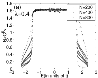
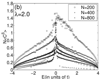
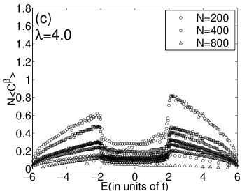
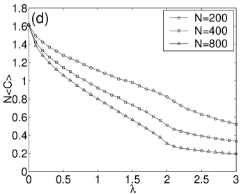
Figure 1: Average concurrence $N\left\langle{C^{\beta}}\right\rangle$ of the individual state in the slowly varying potential model as functions of energy, with $\pi\alpha=0.2$ and $\upsilon=0.7$, (a) $\lambda=0.4$, (b) $\lambda=2.0$ and (c) $\lambda=4.0$, respectively. (d) Average concurrence $N\left\langle{C}\right\rangle$ over all states varying with $\lambda$.

For $0<\upsilon<1$, it is well known that there are two mobility edges at $E_{c}=\pm(2.0-\lambda)$ provided that $\lambda<2.0$. It was found extended states in the middle of the band ( $\left|E\right|<2.0-\lambda$ ) and localized states at the band edge ( $2.0-\lambda<\left|E\right|<2.0+\lambda$ ). For $\lambda>2.0$, all states are found to be localized.

Concurrence $N\left\langle C^{\beta}\right\rangle$ are plotted in Fig.1(a), (b), (c) for $\lambda=0.4,2.0$ and $4.0$ respectively. From Fig.1(a), (b), it’s clearly shown that there are sharp transitions in concurrence at the mobility edges $E_{c}=\pm(2.0-\lambda)$. The transition becomes sharper when $N$ increasing. At extended states, $N\left\langle{C^{\beta}}\right\rangle\approx 1.6$. At the localized states, $N\left\langle{C^{\beta}}\right\rangle$ is decreasing from mobility edges to band top (or bottom). In Fig.1 (c), all states are localized and $N\left\langle{C^{\beta}}\right\rangle$ are small for all states, which is smaller than 1.6. Comparing with Fig.1(a), (b) and (c) in Ref.sa88 , we can found that the longer the localized length is, the larger concurrence is.

The concurrence $N\left\langle{C}\right\rangle$ averaged over all states is plotted in Fig.1(d). There is a transition at $\lambda=2.0$. The transition becomes sharper when $N$ increasing. Obviously there is dramatically transition as $N\rightarrow\infty$ at $\lambda=2.0$.

III.2 Random-dimer potential

Another interesting 1D model, which has localized and extended states, is random-dimer model du90 . In this model, the site energies $V_{a}$ and $V_{b}$ are assigned at random to $2n$th ($n$=integer) site with probability $q$ and $1-q$, and $V_{2n+1}=V_{2n}$. By solving the time-depended Schrödinger equation, Dunlap et al. du90 found that the mean-square displacement at long times is shown to grow in time as $t^{3/2}$ provided $-2<V_{a}-V_{b}<2$, diffusion occurs if $V_{a}-V_{b}=\pm 2$ and localization otherwise. These mean that extended states exist when $-2<V_{a}-V_{b}<2$, and there are only localized states when $|V_{a}-V_{b}|>2$.

Concurrence $N\left\langle C^{\beta}\right\rangle$ are plotted in Fig.2(a), (b), (c) for $V_{a}-V_{b}=1.0$, $2.0$ and $2.5$ respectively. The $V_{b}$ is taken as $1.0$ without loss of generality and $q$ is equal to $0.5$ corresponding to most random situation. The results of Fig.2 are obtained for average of 200 samples gl04 . The averages with more samples give same results. There are two bumps in concurrence when $V_{a}-V_{b}=1.0$. There is no obvious mobility edge in this model, so there is no sharp transition in concurrence as that in the slowly varying potential model. There are two jumps in concurrence when $V_{a}-V_{b}=2.0$. For $V_{a}-V_{b}=2.5$, concurrences are small for all states.

Average concurrence $N\left\langle C\right\rangle$ as functions of $V_{a}-V_{b}$ is plotted in Fig.2(d). There is a jump in the concurrence at $V_{a}-V_{b}=2.0$, which is in accordance with the critical value of $V_{a}-V_{b}$ obtained by dynamical method.

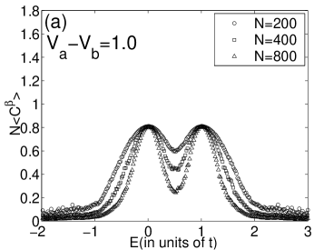
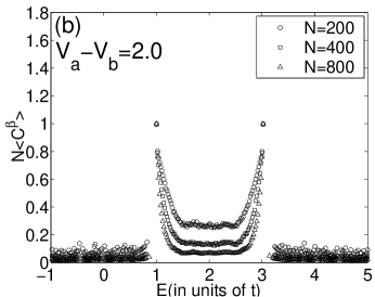
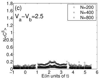
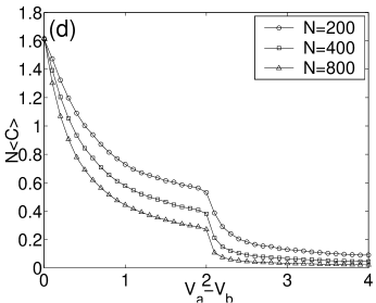
Figure 2: Average concurrence $N\left\langle{C^{\beta}}\right\rangle$ of the individual state in the random-dimer model as functions of energy, (a) $V_{a}-V_{b}=1.0$, (b) $V_{a}-V_{b}=2.0$ and (c) $V_{a}-V_{b}=2.5$, respectively. (d) Average concurrence $N\left\langle{C}\right\rangle$ over all states in the dimer model as functions of $V_{a}-V_{b}$.

III.3 Long-range correlated disordered potential

Recently, another kinds of disordered potential is studied extensively. The potential is self-affine Gaussian potential with Hurst exponent $0<H<1$, such that $<(V_{m}-V_{n})^{2}>=\Delta^{2}\left|{m-n}\right|^{2H}$. Such sequence of potential can be generated by fractional Brownian motion. To generate the trace of a fractional Brownian motion, an approach based on the use of discrete Fourier transforms to construct such long-range correlated sequences can be applied. The on-site energies can be given by the relationmo98 :

$$V_{i}=\sum\limits_{k=1}^{N/2}{[k^{-\alpha}\left|{\frac{{2\pi}}{N}}\right|^{(1-\alpha)}]}^{1/2}\cos(\frac{{2\pi ik}}{N}+\varphi_{k}),$$ (8)

where $N$ is the number of sites and $\varphi_{k}$ are $N/2$ independent random phases uniformly distributed in the interval $[0,2\pi]$. The sequence usually has an approximate power-law spectral density of the form $S(k)\propto 1/k^{\alpha}$, where $S(k)$ is the Fourier transform of the two-point correlation $<V_{i}V_{j}>$. Here $\alpha=2H+1$. Same as in Ref. mo98 , we normalized the energy sequence to have $<V_{n}>=0$ and $\Delta V=\sqrt{\left\langle{V_{n}^{2}}\right\rangle-\left\langle{V_{n}}\right\rangle^{2}}=1$.

It is shown mo98 that when $\alpha<2.0$, all states are localized; when $\alpha>2.0$, localized states occur in the edges of the band and the extended states in the middle of the band, separated by mobility edge.

The relations between concurrence $N\left\langle C^{\beta}\right\rangle$ and eigenenergy $E$ are plotted in Fig.3(a), (b) and (c) for $\alpha=5.0,2.0$ and $1.0$ respectively. Here 200 samples of random $\varphi_{k}$ are averaged. For $\alpha=5.0$, $N\left\langle C^{\beta}\right\rangle\approx 1.6$ in the middle states and $N\left\langle C^{\beta}\right\rangle$ is gradually decreasing from center to band top (or band bottom). The eigenenergies region of extended states is decreasing as $\alpha$ becomes smaller mo98 . When $\alpha=2.0$, the concurrence is near $1.6$ only at band center, which is shown clearly in inset of Fig.3(b). When $\alpha=1.0$, concurrence for all states is small, which corresponds to localized states.

Concurrence averaged over all states is plotted in Fig.3(d). There is an inflexion when $\alpha$ is near $2.0$ in the figure. Same as in model with slowly varying potential, the bigger $N$ is, the transition is sharper.

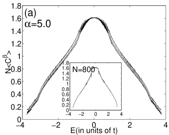
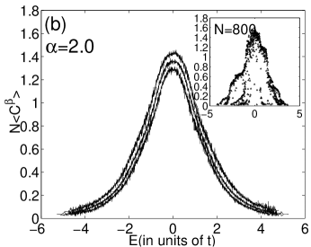
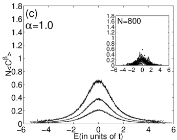
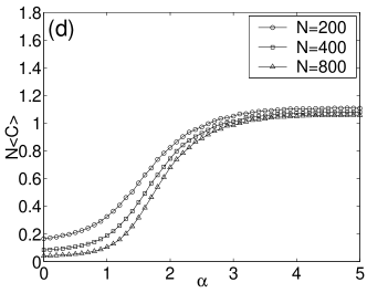
Figure 3: Average concurrence $N\left\langle{C^{\beta}}\right\rangle$ of the individual state in the long-range correlated disordered potential model as functions of energy for (a) $\alpha=5.0$, (b) $\alpha=2.0$ and (c) $\alpha=1.0$, respectively. The insets show concurrence for a typical disorder realization at N=800. (d) Average concurrence $N\left\langle{C}\right\rangle$ over all states as functions of $\alpha$. In all figures, from up to low, $N=200$, $400$ and $800$.

III.4 Random potential with long-range hopping

The random potential with long-range hopping has received considerable attention recently. The Hamiltonian of such 1D tight-binding model is expressed as

$$H=\sum\limits_{n}{\varepsilon_{n}}\left|n\right\rangle\left\langle n\right|+\sum\limits_{n\neq m}{J_{mn}}\left|n\right\rangle\left\langle m\right|,$$ (9)

where $\varepsilon_{n}$ is energy level at nth site , uniformly distributed in interval $[-W/2,W/2]$ and $J_{mn}=J/\left|{m-n}\right|^{\mu}$ ($J_{mm}\equiv 0$) is the long-range hopping amplitude. We will adopt $J$ as energy units without loss of generality. The periodic boundary condition is applied.

By using a supersymmetric method combined with a renormalization group analysis, Rodriguez et al. ro03 have shown the existence of extended states for energies within a range near the band top in one and two dimensional Anderson models. They found that MIT occurs only within the range of $d<\mu<3d/2$ in the thermodynamic limit, no matter how large the value of $W$ is, here $d$ is the geometric dimensionality of the system. Using finite size scaling analysis combined with the transfer matrix method, Xiong and Zhang xi03 found that there exists MIT at critical value $\mu_{c}$ for some $W$.

The concurrence $N\left\langle C^{\beta}\right\rangle$ as functions of energy are plotted in Fig.4 (a), (b) and (c) for $\mu=1.1$, $1.5$ and $1.7$ respectively. Here $W=5$ is taken as example and the phenomena are similar for other $W$. The results are obtained for average of $200,100,50$ samples gl04 for $N=200,400,800$ respectively. When $\mu=1.1$ and $1.5$, concurrence $N\left\langle C^{\beta}\right\rangle$ is large for states near the band top, which means there exist extended states. It is small for the states near the band bottom. This is quite different from that of above three models. For $\mu=1.7$, the concurrence is small for all states, which means all states are localized.

The concurrence averaged over all states is plotted in Fig.4(d). From the inset, we can get the inflexion for $\mu$ near $1.70$, which is consistence with the upper limit for critical value $\mu_{c}$ obtained in Ref.xi03 .

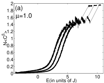
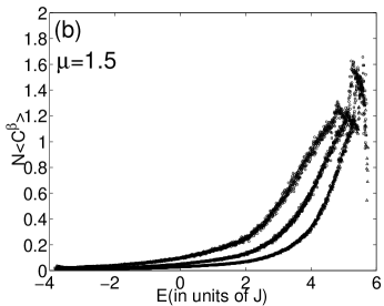
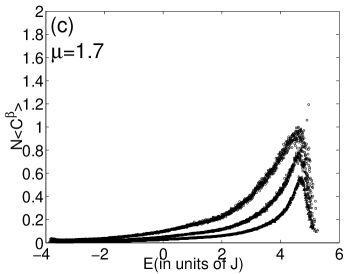
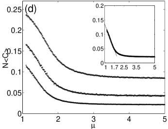
Figure 4: Average concurrence $N\left\langle{C^{\beta}}\right\rangle$ of the individual state in the model with long-range hopping as functions of energy, with $W=5.0$, (a) $\mu$=1.1, (b) $\mu=1.5$ and (c) $\mu=1.7$, respectively. (d)Average concurrence $N\left\langle{C}\right\rangle$ over all states as functions of $\mu$. The inset shows concurrence when $N=800$. The line is linear fitted line for $\mu<1.5$ . In all figures, from up to low, $N=200,400,800$.

IV Conclusion

Using the measure of concurrence, mode entanglement sharing in one-particle states in four kinds of models is studied numerically. Concurrence $N\left\langle C^{\beta}\right\rangle$ at a given state and $N\left\langle C\right\rangle$ averaged over all states are investigated. For $N\left\langle C^{\beta}\right\rangle$, the concurrence is large in extended states and small in localized states. There is a sharp transition in the concurrence at mobility edge. $N\left\langle C^{\beta}\right\rangle$ gives the information about the localization behavior of the given eigenstate $\beta$. From the curves of the $N\left\langle C\right\rangle$ vs the parameter of the models, which is $\lambda$, $V_{a}-V_{b}$, $\alpha$, and $\mu$ for slowly varying potential, random-dimer potential, long-range correlated disordered potential, and long-range hopping random potential, respectively, we can found clearly that there is an inflexion (or jump) at a critical parameter value, which is in accordance with that obtained by other methods. When parameter value is greater (smaller) than the critical parameter value, the system has only localized eigenstates, while when parameter value is smaller (greater) than the critical parameter value, the system has both localized and delocalized states, which is different from that of one-dimensional Harper model. The inflexion or transition point in the curve of $N\left\langle C\right\rangle$ versus parameter of systems corresponds to the disappear of delocalized states. Therefore mode entanglement can be a new index to reflect MIT.

- (1) E. Schrödinger, Proc. Cambridge Philos. Soc. 31, 555 (1935); J. S. Bell, Physics, 1, 195 (1964).
- (2) See, for example, The Physics of Quantum Information, Eds., D. Bouwmeester, A. Ekert, and A. Zeilinger,(Springer, Berlin 2000).
- (3) C. H. Bennett, D. P. DiVincenzo, J. A. Smolin, and W. K. Wootters, Phys. Rev. A 54, 3824 (1996).
- (4) C. H. Bennett, G. Brassard, S. Popescu, B. Schumacher, J. A. Smolin, and W. K. Wootters, Phys. Rev. Lett. 76, 722 (1996).
- (5) W. K. Wootters, Quamt. Inf. and Comp. 1 27 (2001).
- (6) S. Hill, and W. K. Wootters, Phys. Rev. Lett. 78, 5022 (1997); W. K. Wootters, Phys. Rev. Lett. 80, 2245 (1998).
- (7) G. Vidal, J. I. Latorre, E. Rico, and A. Kitaev, Phys. Rev. Lett. 90, 227902 (2003).
- (8) U. Glaser, H. Büttner, and H. Fehske, Phys. Rev. A 68, 032318 (2003).
- (9) J. Schliemann, J. I. Cirac, M. Kus, M.Lewenstein and D. Loss, Phys. Rev. A 64, 022303 (2001).
- (10) H. M. Wiseman and J. A. Vaccaro, Phys. Rev. Lett. 91, 097902 (2003).
- (11) B. Zeng, H. Zhai, and Z. Xu, Phys. Rev. A 66, 042324 (2002).
- (12) S. Oh and J. Kim, Phys. Rev. A 69, 054305 (2004).
- (13) P. W. Anderson, Phys. Rev. 109, 1429 (1958).
- (14) T. V. Ramakrishnan and P. A. Lee, Rev. Mod. Phys. 57, 287 (1985).
- (15) M. Griniasty and S. Fishman, Phys. Rev. Lett. 60, 1334 (1988).
- (16) D. J. Thouless, Phys. Rev. Lett. 61, 2141 (1988).
- (17) S. Das Sarma, S. He, and X. C. Xie, Phys. Rev. Lett. 61 2144 (1988).
- (18) D. H. Dunlap, H-L. Wu and P. W. Phillips, Phys. Rev. Lett. 65, 88 (1990).
- (19) F. A. B. F. de Moura and M. L. Lyra, Phys. Rev. Lett.81 3735 (1998).
- (20) A. Rodríguez, V. A. Malyshev, G. Sierra, M. A. Martín-Delgado, J. Rodríguez-Laguna, and F. Domínguez-Adame, Phys. Rev. Lett. 90, 027404 (2003).
- (21) S. J. Xiong and G. P. Zhang, Phys. Rev. B 68 174201 (2003).
- (22) A. Lakshminarayan and V. Subrahmanyam, Phys. Rev. A 67, 052304 (2003).
- (23) X. Wang, H. Li, and B. Hu, Phys. Rev. A 69, 054303 (2004).
- (24) W. Dür, G. Vidal, and J. I. Cirac, Phys. Rev. A 62, 062314 (2000).
- (25) For random potentials, we use the following definition of concurrence:, here is denoted as random average, is the number samples, and denotes a given state.