On the conditional logistic estimator
for repeated binary outcomes
in two-arm experimental studies with non-compliance

Francesco Bartolucci111 Department of Economics, Finance and Statistics, University of Perugia, 06123 Perugia, Italy, email: bart@stat.unipg.it
Abstract

The behavior of the conditional logistic estimator is analyzed under a causal model for two-arm experimental studies with possible non-compliance in which the effect of the treatment is measured by a binary response variable. We show that, when non-compliance may only be observed in the treatment arm, the effect (measured on the logit scale) of the treatment on compliers and that of the control on non-compliers can be identified and consistently estimated under mild conditions. The same does not happen for the effect of the control on compliers. A simple correction of the conditional logistic estimator is then proposed which allows us to considerably reduce its bias in estimating this quantity and the causal effect of the treatment over control on compliers. A two-step estimator results whose asymptotic properties are studied by exploiting the general theory on maximum likelihood estimation of misspecified models. Finite-sample properties of the estimator are studied by simulation and the extension to the case of missing responses is outlined. The approach is illustrated by an application to a dataset deriving from a study on the efficacy of a training course on the practise of breast self examination.

Key words: Causal inference; Counterfactuals; Potential outcomes; Pseudo-likelihood inference; Sufficient statistics.

1 Introduction

Conditional logistic regression is a commonly used tool of data analysis in the health sciences and medical statistics when the outcome of interest is binary and subjects are observed before and after a certain treatment or these subjects are somehow matched; see, for instance, [1], [2], [3] and [4]. The main reasons of the popularity of the method are represented by its simplicity and by the possibility of obtaining reliable estimates of the quantities of interest under very mild conditions.

The first aim of this paper is that of illustrating the behavior of the conditional logistic estimator when data come from two-arm experimental studies with all-or-nothing compliance in which the efficacy of the treatment is observed through a binary variable, and a pre-treatment version of the same variable is available. We are then in a context of repeated binary outcomes at two occasions, before and after the treatment (or control), for which non-compliance may represent a strong source of confounding in estimating the causal effect of the treatment over control. An example is represented by the study described by [5] on the effect of a training course on the attitude to practise breast self examination (BSE); see also [6]. In this study, a significant number of women, among those randomly assigned to the treatment, did not comply and preferred learning BSE by a standard method (control). Moreover, the efficacy of the treatment is measured by a binary variable indicating if a women regularly practises BSE and another binary variable indicating if BSE is practised in the proper way (provided it is practised). Pre-treatment values of these response variables are also available.

In order to study the behavior of the conditional logistic estimator in experimental studies of the type described above, we introduce a causal model which includes parameters for the control and treatment effects in the subpopulation of compliers and never-takers and assumes that only the subjects assigned to the treatment can access it. Given the type of experimental studies, we assume that always-takers do not exist; we also assume that defiers are no present. The model is then related to the causal models described by [7] and [8]; see also [9]. It also allows for the inclusion of base-line observable and unobservable covariates which affect the response variables at the first and second occasions. We show that, under this model, the conditional logistic method allows us to identify and consistently estimate the effect of the treatment on compliers and that of the control on never-takers. However, apart from very particular cases, this method does not allow us to identify the effect of control on the subpopulation of compliers and then the causal effect of the treatment over control on this subpopulation. As in other approaches for causal inference, this effect is here measured on the logit scale; see [10], [11], [12] and [13].

Based on an approximation of the distribution of the observable variables under the causal model, we then propose a correction for the conditional logistic estimator which allows us to remove most of its bias in estimating the effect of the treatment on compliers. It results a two-step estimator which has some connection with the estimator usually adopted for the selection model [14] and that proposed by [15] to estimate the causal effect of a treatment in a context similar to the present one. At the first step, the parameters of a model for the probability that a subject is a complier are estimated. At the second step, a conditional logistic likelihood is maximized which is based on an approximated version of the conditional probability of the response variables at the two occasions, given their sum. This likelihood is computed on the basis of the first step parameter estimates. The proposed estimator is very simple to use and is consistent when the control has the same effect on compliers and never-takers. This result holds regardless of the model that we choose for the probability to comply. In the general case in which compliers and never-takers react differently to control, the estimator is not consistent but we show that it may converge in probability to a value surprisingly close to the true value of the causal parameters as the sample size grows to infinity. We also derive a sandwich formula for its standard error. As we show, with minor adjustments the two-step estimator leads to valid inference even with missing responses.

The paper is organized as follows. In Section 2 we introduce the causal model for repeated outcomes coming from two-arm experimental studies. The behavior of the conditional logistic estimator under this model is studied in Section 3. The correction of this estimator is proposed in Section 4 where we also study the asymptotic and finite-sample properties of the resulting two-step estimator. In Section 5 we outline the extension of the approach to missing responses and in Section 6 we provide an illustration based on an application to the dataset deriving from the BSE study described above. Final conclusions are reported in Section 7 where possible extensions are also mentioned, such us that to experimental studies in which subjects in both arms can access the treatment and then non-compliance phenomena can be observed for all subjects.

2 The causal model

Let $Y_{1}$ and $Y_{2}$ denote the binary response variables of interest, let $V$ be a vector of observable covariates, let $Z$ be a binary variable equal to 1 when a subject is assigned to the treatment and to 0 when he/she is assigned to the control and let $X$ be the corresponding binary variable for the treatment actually received. We recall that $V$ and $Y_{1}$ are pre-treatment variables, whereas $Y_{2}$ is a post-treatment variable. Non-compliance of the subjects involved in the experimental study implies that $X$ may differ from $Z$. In particular we consider experiments in which only subjects randomized to the treatment can access it and therefore $Z=0$ implies $X=0$, whereas with $Z=1$ we may observe either $X=0$ or $X=1$. Using a terminology taken from [7], in this case we have only randomized eligibility and we then consider two subpopulations: compliers and never-takers. Nevertheless, the approach can be extended to randomized experiments in which subjects in both arms can access the treatment and therefore any configuration of $(Z,X)$ may be observed; see Section 7 for a discussion on this point. In both types of experiment, we assume that defiers are not present and our aim is that of estimating the causal effect of the treatment over control in the subpopulation of compliers.

We assume that the behaviour of a subject depends on the observable covariates $V$, a latent variable $U$ representing the effect of unobservable covariates on both response variables and a latent variable $C$ representing the attitude to comply with the assigned treatment. The last one, in particular, is a discrete variable with two levels: 0 for never-takers, 1 for compliers.

The model is based on the following assumptions:

  • A1:

    Cβ€‹βŠ§β€‹Y1|(U,𝑽)conditional𝐢⊧subscriptπ‘Œ1π‘ˆπ‘½C\>\begin{sideways}$\models$\end{sideways}\>Y_{1}|(U,\mbox{\boldmath$V$}), i.e. C𝐢C is conditionally independent of Y1subscriptπ‘Œ1Y_{1} given (U,𝑽)π‘ˆπ‘½(U,\mbox{\boldmath$V$});

  • A2:

    Zβ€‹βŠ§β€‹(U,Y1,C)|𝑽conditionalπ‘βŠ§π‘ˆsubscriptπ‘Œ1𝐢𝑽Z\>\begin{sideways}$\models$\end{sideways}\>(U,Y_{1},C)|\mbox{\boldmath$V$};

  • A3:

    Xβ€‹βŠ§β€‹(U,𝑽,Y1)|(C,Z)conditionalπ‘‹βŠ§π‘ˆπ‘½subscriptπ‘Œ1𝐢𝑍X\>\begin{sideways}$\models$\end{sideways}\>(U,\mbox{\boldmath$V$},Y_{1})|(C,Z) and, with probability 1, X=Z𝑋𝑍X=Z when C=1𝐢1C=1 (compliers) and X=0𝑋0X=0 when C=0𝐢0C=0 (never-takers);

  • A4:

    Y2β€‹βŠ§β€‹(Y1,Z)|(U,𝑽,C,X)conditionalsubscriptπ‘Œ2⊧subscriptπ‘Œ1π‘π‘ˆπ‘½πΆπ‘‹Y_{2}\>\begin{sideways}$\models$\end{sideways}\>(Y_{1},Z)|(U,\mbox{\boldmath$V$},C,X);

  • A5:

    for any $u,\mbox{\boldmath$v$},c$ and $x$, we have

    $${\rm logit}[p(Y_{2}=1|u,\mbox{\boldmath$v$},c,x)]-{\rm logit}[p(Y_{1}=1|u,\mbox{\boldmath$v$})]=\mbox{\boldmath$a$}(\mbox{\boldmath$v$},x)^{\prime}\mbox{\boldmath$\alpha$}+c(1-x)\mbox{\boldmath$b$}(\mbox{\boldmath$v$})^{\prime}\mbox{\boldmath$\beta$},$$ (1)

    where $\mbox{\boldmath$a$}(\mbox{\boldmath$v$},x)$ and $\mbox{\boldmath$b$}(\mbox{\boldmath$v$})$ are known functions which depend on observable covariates and (limited to the first) on the received treatment and $\alpha$ and $\beta$ are corresponding vectors of parameters.

The above assumptions lead to a dependence structure on the observable and unobservable variables which is represented by the DAG in Figure 1.

Refer to caption
Figure 1: DAG for the model based on assumptions A1-A5. $U$ and $V$ represent unobservable and observable covariates affecting the response variables $Y_{1}$ and $Y_{2}$, $C$ is a binary variable for the compliance status and $Z$ and $X$ are binary variables for the assigned and received treatment.

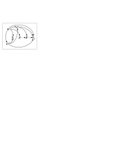
Assumption A1 says that the tendency to comply only depends on $(U,\mbox{\boldmath$V$})$. Assumption A2 is satisfied in randomized experiments, even when randomization is conditioned on the observable covariates. This assumption could be relaxed by requiring that $Z$ is conditionally independent of $U$ given $(\mbox{\boldmath$V$},Y_{1})$, so that randomization can also be conditioned on the first outcome. Assumption A3 is rather obvious considering that $C$ represents the tendency of a subject to comply with the assigned treatment. Assumption A4 implies that there is no direct effect of $Y_{1}$ on $Y_{2}$, since the distribution of the latter only depends on $(U,\mbox{\boldmath$V$},C,X)$. Using a terminology which is well known in the literature on latent variable models, this is an assumption of local independence. Assumption A4 also implies an assumption known in the causal inference literature as exclusion restriction, according to which $Z$ affects $Y_{2}$ only through $X$. Finally, assumption A5 says that the distribution of $Y_{2}$ depends on the vectors of parameters $\alpha$ and $\beta$ through the functions $\mbox{\boldmath$a$}(\mbox{\boldmath$v$},x)$ and $\mbox{\boldmath$b$}(\mbox{\boldmath$v$})$. Note, in particular, that $\mbox{\boldmath$a$}(\mbox{\boldmath$v$},0)^{\prime}\mbox{\boldmath$\alpha$}$ is the effect of the control on never-takers, $\mbox{\boldmath$a$}(\mbox{\boldmath$v$},1)^{\prime}\mbox{\boldmath$\alpha$}$ is the effect of the treatment on compliers, whereas $\mbox{\boldmath$b$}(\mbox{\boldmath$v$})^{\prime}\mbox{\boldmath$\beta$}$ is the differential effect of the control between compliers and never-takers. In the simplest case, we have

$$\mbox{\boldmath$a$}(\mbox{\boldmath$v$},x)=(1-x,x)^{\prime}\quad\mbox{and}\quad b(\mbox{\boldmath$v$})=1,$$ (2)

so that $\mbox{\boldmath$\alpha$}=(\alpha_{1},\alpha_{2})^{\prime}$ and $\beta$ have an obvious interpretation as effects of the control and the treatment on specific subpopulations.

As mentioned above, the most interest quantity to estimate is the causal effect of the treatment over the control in the subpopulation of compliers. In the present approach, this effect is defined as the difference in logits (log-odds ratio)

$\displaystyle\delta(\mbox{\boldmath$v$})$ $\displaystyle=$ $\displaystyle{\rm logit}[p(Y_{2}=1|u,\mbox{\boldmath$v$},C=1,X=1)]-{\rm logit}[p(Y_{2}=1|u,\mbox{\boldmath$v$},C=1,X=0)]=$ (3)
$\displaystyle=$ $\displaystyle[\mbox{\boldmath$a$}(\mbox{\boldmath$v$},1)-\mbox{\boldmath$a$}(\mbox{\boldmath$v$},0)]^{\prime}\mbox{\boldmath$\alpha$}-\mbox{\boldmath$b$}(\mbox{\boldmath$v$})^{\prime}\mbox{\boldmath$\beta$},$

and, with reference to the subpopulation of compliers, it corresponds to the increase of the logit of the probability of success when $X$ goes from 0 to 1, all the other factors remaining unchanged. This quantity depends on the covariates in $V$ and then an overall causal effect can be computed as the average of $\delta(\mbox{\boldmath$v$})$ over suitable configurations of these covariates. Under (2), we simply have $\delta=\alpha_{2}-\alpha_{1}-\beta$ and then computing this average is not necessary. Also note that the model makes sense, not only when $Y_{1}$ is a response variable of the same nature of $Y_{2}$ that is observed before the treatment, but also when $Y_{1}$ is a variable which is affected neither by the compliance status nor by the treatment received and such that the difference between the logits in (1) is independent of $u$ and $v$.

That based on assumptions A1-A5 is a causal model in the sense of [16] since all the observable and unobservable factors affecting the response variables of interest are included. Indeed, the same model could be formulated by exploiting potential outcomes, which we denote by $Y_{2}^{(z,x)}$, $z,x=0,1$. In this case, the model could be formulated on the basis of assumptions A1-A3 and the following assumptions which substitute A4-A5:

  • A4βˆ—:

    Y2(z,x)=Y2(x)superscriptsubscriptπ‘Œ2𝑧π‘₯superscriptsubscriptπ‘Œ2π‘₯Y_{2}^{(z,x)}=Y_{2}^{(x)} for z,x=0,1formulae-sequence𝑧π‘₯01z,x=0,1 (exclusion restriction) and (Y2(0),Y2(1))β€‹βŠ§β€‹(Y1,Z,X)|(U,𝑽,C)conditionalsuperscriptsubscriptπ‘Œ20superscriptsubscriptπ‘Œ21⊧subscriptπ‘Œ1π‘π‘‹π‘ˆπ‘½πΆ(Y_{2}^{(0)},Y_{2}^{(1)})\>\begin{sideways}$\models$\end{sideways}\>(Y_{1},Z,X)|(U,\mbox{\boldmath$V$},C);

  • A5βˆ—:

    for any $u,\mbox{\boldmath$v$},c$ and $x$, we have

    $${\rm logit}[p(Y_{2}^{(x)}=1|u,\mbox{\boldmath$v$},c)]-{\rm logit}[p(Y_{1}=1|u,\mbox{\boldmath$v$})]=\mbox{\boldmath$a$}(\mbox{\boldmath$v$},x)^{\prime}\mbox{\boldmath$\alpha$}+c(1-x)\mbox{\boldmath$b$}(\mbox{\boldmath$v$})^{\prime}\mbox{\boldmath$\beta$};$$ (4)
  • A6βˆ—:

    $Y_{2}=Y_{2}^{(x)}$ for any given value of $U,\mbox{\boldmath$V$},C$ and any given value $x$ of $X$.

It may be easily realized that the model based on assumptions A1-A5 is equivalent to that based on assumptions A1-A3 and A4βˆ—-A6βˆ—. In a similar context, this kind of equivalence between causal models is dealt with by [10].

It is even more clear from (4) that $\alpha$ and $\beta$ are vectors of causal parameters, in the sense that they allow us to measure the causal effect of the treatment over control in the subpopulation of compliers. Using potential outcomes and for simplicity under (2), this effect may now be expressed as

$$\delta={\rm logit}[p(Y_{2}^{(1)}=1|u,\mbox{\boldmath$v$},C=1)]-{\rm logit}[p(Y_{2}^{(0)}=1|u,\mbox{\boldmath$v$},C=1)]=\alpha_{2}-\alpha_{1}-\beta.$$

3 Behavior of the conditional logistic estimator

In this section we show that, by the conditional logistic method and under mild conditions, we can identify and consistently estimate the parameter vector $\alpha$ which measures the effect of the treatment on compliers and that of the control on never-takers. However, the same is not possible for $\beta$. In order to show this we need to derive the conditional distribution of $(Y_{1},Z,X,Y_{2})$ given $V$ under the assumptions introduced in Section 2. The probability mass function of this distribution is denoted by $f(y_{1},z,x,y_{2}|\mbox{\boldmath$v$})$.

First of all, these assumptions imply that the probability function of the conditional distribution of $(Y_{1},Z,X,Y_{2})$ given $(U,\mbox{\boldmath$V$},C)$ is equal to

$$p(y_{1},z,x,y_{2}|u,\mbox{\boldmath$v$},c)=p(y_{1}|u,\mbox{\boldmath$v$})p(z|\mbox{\boldmath$v$})p(x|c,z)p(y_{2}|u,\mbox{\boldmath$v$},c,x).$$

After some algebra we have

$$p(y_{1},z,x,y_{2}|u,\mbox{\boldmath$v$})=\frac{e^{(y_{1}+y_{2})\lambda(u,\mbox{\footnotesize\boldmath{$v$}})}}{1+e^{\lambda(u,\mbox{\footnotesize\boldmath{$v$}})}}p(z|\mbox{\footnotesize\boldmath{$v$}})\sum_{c}p(x|c,z)\frac{e^{y_{2}t(c,\mbox{\footnotesize\boldmath{$v$}},x)}}{1+e^{\lambda(u,\mbox{\footnotesize\boldmath{$v$}})+t(c,\mbox{\footnotesize\boldmath{$v$}},x)}}\pi(c|u,\mbox{\boldmath$v$}),$$

where $\lambda(u,\mbox{\boldmath$v$})={\rm logit}[p(Y_{1}=1|u,\mbox{\boldmath$v$})]$, $\pi(c|u,\mbox{\boldmath$v$})=p(c|u,\mbox{\boldmath$v$})$ and the sum $\sum_{c}$ is extended to $c=0,1$. Moreover, $t(c,\mbox{\boldmath$v$},x)=\mbox{\boldmath$a$}(\mbox{\boldmath$v$},x)^{\prime}\mbox{\boldmath$\alpha$}+c(1-x)\mbox{\boldmath$b$}(\mbox{\boldmath$v$})^{\prime}\mbox{\boldmath$\beta$}$; see equation (1). Finally, denoting by $\phi(u|\mbox{\boldmath$v$})$ the density function of the conditional distribution of $U$ given $V$ and letting $y_{+}=y_{1}+y_{2}$, we have

$$f(y_{1},z,x,y_{2}|\mbox{\boldmath$v$})=p(z|\mbox{\boldmath$v$})\int\frac{e^{y_{+}\lambda(u,\mbox{\footnotesize\boldmath{$v$}})}}{1+e^{\lambda(u,\mbox{\footnotesize\boldmath{$v$}})}}\sum_{c}p(x|c,z)\frac{e^{y_{2}t(c,\mbox{\footnotesize\boldmath{$v$}},x)}}{1+e^{\lambda(u,\mbox{\footnotesize\boldmath{$v$}})+t(c,\mbox{\footnotesize\boldmath{$v$}},x)}}\pi(c|u,\mbox{\boldmath$v$})\phi(u|\mbox{\boldmath$v$})du.$$ (5)

When $z=1$ (treatment arm), $p(x|c,z)$ is equal to 1 for $x=c$ and to 0 otherwise. Consequently, (5) reduces to

$$f(y_{1},1,x,y_{2}|\mbox{\boldmath$v$})=p(Z=1|\mbox{\boldmath$v$})\int\frac{e^{y_{+}\lambda(u,\mbox{\footnotesize\boldmath{$v$}})}}{1+e^{\lambda(u,\mbox{\footnotesize\boldmath{$v$}})}}\frac{e^{y_{2}\mbox{\footnotesize\boldmath{$a$}}(\mbox{\footnotesize\boldmath{$v$}},x)^{\prime}\mbox{\footnotesize\boldmath{$\alpha$}}}}{1+e^{\lambda(u,\mbox{\footnotesize\boldmath{$v$}})+\mbox{\footnotesize\boldmath{$a$}}(\mbox{\footnotesize\boldmath{$v$}},x)^{\prime}\mbox{\footnotesize\boldmath{$\alpha$}}}}\pi(x|u,\mbox{\footnotesize\boldmath{$v$}})\phi(u|v)du,$$ (6)

since it is possible to identify a subject in this arm as a never-taker or a compiler according to whether $x=0$ or $x=1$ and $t(c,\mbox{\boldmath$v$},x)=\mbox{\boldmath$a$}(\mbox{\boldmath$v$},x)^{\prime}\mbox{\boldmath$\alpha$}$ when $c=x$. Now let $f(y_{2}|\mbox{\boldmath$v$},z,x)$ denote the probability mass function of the conditional distribution of $Y_{2}$ given $(\mbox{\boldmath$V$},X,Y_{+}=1)$, with $Y_{+}=Y_{1}+Y_{2}$. The above result implies that

$$f(y_{2}|\mbox{\boldmath$v$},1,x)=\frac{f(1-y_{2},1,x,y_{2}|v)}{f(0,1,x,1|v)+f(1,1,x,0|v)}=\frac{e^{y_{2}\mbox{\footnotesize\boldmath{$a$}}(\mbox{\footnotesize\boldmath{$v$}},x)^{\prime}\mbox{\footnotesize\boldmath{$\alpha$}}}}{1+e^{\mbox{\footnotesize\boldmath{$a$}}(\mbox{\footnotesize\boldmath{$v$}},x)^{\prime}\mbox{\footnotesize\boldmath{$\alpha$}}}}.$$ (7)

This probability function depends neither on the distribution of $U$ nor on the function $\lambda(u,\mbox{\boldmath$v$})$. Consequently, as already mentioned above, we can identify the parameters in $\alpha$ measuring the effect of the treatment on compliers and that of the control on never-takers and the conditional logistic estimator of these parameters is consistent. It is also worth to observe that under assumption (2), which implies that $\mbox{\boldmath$\alpha$}=(\alpha_{1},\alpha_{2})^{\prime}$, the conditional logistic estimator of these parameters has an explicit form given by

$$\hat{\alpha}_{1}=\log\frac{n_{0101}}{n_{1100}}\quad\mbox{and}\quad\hat{\alpha}_{2}=\log\frac{n_{0111}}{n_{1110}},$$

where $n_{y_{1}zxy_{2}}$ denotes the number of subjects in the sample with response configuration $(y_{1},y_{2})$ who are in the control or treatment arm (according to whether $z=0$ or $z=1$) and chose or not the treatment (according to whether $x=0$ or $x=1$).

When $z=0$ (control arm), $p(x|c,z)$ is equal to 1 for $x=0$ and to 0 otherwise (regardless of $c$), since no subject in this arm can access the treatment. Then, expression (5) reduces to

$\displaystyle f(y_{1},0,0,y_{2}|\mbox{\boldmath$v$})$ $\displaystyle=$ $\displaystyle p(Z=0|\mbox{\boldmath$v$})g(y_{1},y_{2}|\mbox{\boldmath$v$}),$
$\displaystyle g(y_{1},y_{2}|\mbox{\boldmath$v$})$ $\displaystyle=$ $\displaystyle\int\frac{e^{y_{+}\lambda(u,\mbox{\footnotesize\boldmath{$v$}})}}{1+e^{\lambda(u,\mbox{\footnotesize\boldmath{$v$}})}}\sum_{c}\frac{e^{y_{2}t(c,\mbox{\footnotesize\boldmath{$v$}},0)}}{1+e^{\lambda(u,\mbox{\footnotesize\boldmath{$v$}})+t(c,\mbox{\footnotesize\boldmath{$v$}},0)}}\pi(c|u,\mbox{\boldmath$v$})\phi(u|\mbox{\boldmath$v$})du,$

which is more complex than (6), being based on a mixture between the conditional distribution of $Y_{2}$ for the subpopulation of compliers and for that of never-takers. In this case, we cannot remove the dependence on the distribution of $U$ and on $\lambda(u,\mbox{\boldmath$v$})$ via conditioning on $Y_{+}$. Then, we cannot identify and consistently estimate the parameters in $\beta$ corresponding to the differential effect of control on compliers with respect to never-takers. The same happens for the causal effect $\delta(\mbox{\boldmath$v$})$ defined in (3).

In order to better investigate this point we consider an approximation of $\log g(y_{1},y_{2}|\mbox{\boldmath$v$})$ based on a first-order Taylor series expansion around $\mbox{\boldmath$\beta$}=\mbox{\boldmath$0$}$, with 𝟎0 denoting a column vector of zeros of suitable dimension. Note that this point corresponds to the situation in which the control has the same effect on compliers and never-takers. We have that

$$\log g(y_{1},y_{2}|\mbox{\boldmath$v$})\approx\log g_{0}(y_{1},y_{2}|\mbox{\boldmath$v$})+h(y_{1},y_{2}|\mbox{\boldmath$v$})\mbox{\boldmath$b$}(\mbox{\boldmath$v$})^{\prime}\mbox{\boldmath$\beta$},$$

where $g_{0}(y_{1},y_{2}|\mbox{\boldmath$v$})$ is equal to $g(y_{1},y_{2}|\mbox{\boldmath$v$})$ computed at $\mbox{\boldmath$\beta$}=\mbox{\boldmath$0$}$, that is

$$g_{0}(y_{1},y_{2}|\mbox{\boldmath$v$})=\int\frac{e^{y_{+}\lambda(u,\mbox{\footnotesize\boldmath{$v$}})}}{1+e^{\lambda(u,\mbox{\footnotesize\boldmath{$v$}})}}\frac{e^{y_{2}t(0,\mbox{\footnotesize\boldmath{$v$}},0)}}{1+e^{\lambda(u,\mbox{\footnotesize\boldmath{$v$}})+t(0,\mbox{\footnotesize\boldmath{$v$}},0)}}\phi(u|\mbox{\boldmath$v$})du,$$

and

$$h(y_{1},y_{2}|\mbox{\boldmath$v$})=\frac{2y_{2}-1}{g_{0}(y_{1},y_{2}|\mbox{\boldmath$v$})}\int\frac{e^{y_{+}\lambda(u,\mbox{\footnotesize\boldmath{$v$}})}}{1+e^{\lambda(u,\mbox{\footnotesize\boldmath{$v$}})}}\frac{e^{t(0,\mbox{\footnotesize\boldmath{$v$}},0)}}{[1+e^{\lambda(u,\mbox{\footnotesize\boldmath{$v$}})+t(0,\mbox{\footnotesize\boldmath{$v$}},0)}]^{2}}\pi(1|u,\mbox{\boldmath$v$})\phi(u|\mbox{\boldmath$v$})du.$$

Now, because $g_{0}(0,1|\mbox{\boldmath$v$})=g_{0}(1,0|\mbox{\boldmath$v$})e^{t(0,\mbox{\footnotesize\boldmath{$v$}},0)}$ and recalling that $t(0,\mbox{\boldmath$v$},0)=\mbox{\boldmath$a$}(\mbox{\boldmath$v$},0)^{\prime}\mbox{\boldmath$\alpha$}$, after some algebra (see Appendix A1 for details) we find

$$\log\frac{f(0,0,0,1|\mbox{\boldmath$v$})}{f(1,0,0,0|\mbox{\boldmath$v$})}=\log g(0,1|\mbox{\boldmath$v$})-\log g(1,0|\mbox{\boldmath$v$})\approx\mbox{\boldmath$a$}(\mbox{\boldmath$v$},0)^{\prime}\mbox{\boldmath$\alpha$}+h(\mbox{\boldmath$v$})\mbox{\boldmath$b$}(\mbox{\boldmath$v$})^{\prime}\mbox{\boldmath$\beta$},$$ (8)

where $h(\mbox{\boldmath$v$})$ is a correction factor defined as

$$h(\mbox{\boldmath$v$})=\frac{1}{g_{0}(1,0|\mbox{\boldmath$v$})}\int\frac{e^{\lambda(u,\mbox{\footnotesize\boldmath{$v$}})}}{1+e^{\lambda(u,\mbox{\footnotesize\boldmath{$v$}})}}\frac{1}{1+e^{\lambda(u,\mbox{\footnotesize\boldmath{$v$}})+t(0,\mbox{\footnotesize\boldmath{$v$}},0)}}\pi(1|u,\mbox{\boldmath$v$})\phi(u|\mbox{\boldmath$v$})du.$$ (9)

This correction term is simply equal to $\pi(1|\mbox{\boldmath$v$})=p(C=1|\mbox{\boldmath$v$})$ when $C$ is conditionally independent of $U$ given $V$. We then have

$$f(y_{2}|\mbox{\boldmath$v$},0,0)=\frac{f(1-y_{2},0,0,y_{2}|\mbox{\boldmath$v$})}{f(0,0,0,1|\mbox{\boldmath$v$})+f(1,0,0,0|\mbox{\boldmath$v$})}\approx\frac{e^{\mbox{\footnotesize\boldmath{$a$}}(\mbox{\footnotesize\boldmath{$v$}},0)^{\prime}\mbox{\footnotesize\boldmath{$\alpha$}}+h(\mbox{\footnotesize\boldmath{$v$}})\mbox{\footnotesize\boldmath{$b$}}(\mbox{\footnotesize\boldmath{$v$}})^{\prime}\mbox{\footnotesize\boldmath{$\beta$}}}}{1+e^{\mbox{\footnotesize\boldmath{$a$}}(\mbox{\footnotesize\boldmath{$v$}},0)^{\prime}\mbox{\footnotesize\boldmath{$\alpha$}}+h(\mbox{\footnotesize\boldmath{$v$}})\mbox{\footnotesize\boldmath{$b$}}(\mbox{\footnotesize\boldmath{$v$}})^{\prime}\mbox{\footnotesize\boldmath{$\beta$}}}}$$ (10)

which shows that a conditional logistic estimator based on regressing $Y_{2}$ on $V$, only for the cases in which $Y_{+}=1$ and $Z=0$, would estimate a quantity which does not correspond to the effect of the control either on compliers or on never-takers.

To clarify the above point consider the case of absence of covariates in which assumption (2) holds. In this case, the conditional logistic estimator is equal to $\log(n_{0001}/n_{1000})$ which converges in probability to a quantity close to $\alpha_{1}+h\beta$. Then, provided that $h$ can be suitably estimated, a correction for this estimator can be implemented so as to reduce its bias. This idea is exploited to propose a general approach which allows us to considerably reduce the bias of the conditional logistic estimator applied to the data coming from the control group.

4 Corrected conditional logistic estimator

With reference to a sample of $n$ subjects included in the two-arm experimental study, let $y_{i1}$ denote the observed value of $Y_{1}$ for subject $i$, let $y_{i2}$ denote the value of $Y_{2}$ for the same subject and let $\mbox{\boldmath$v$}_{i}$, $z_{i}$ and $x_{i}$ denote the corresponding values of $V$, $Z$ and $X$, respectively.

4.1 The estimator

In order to estimate the parameters of the causal model introduced in Section 2, we rely on a standard logistic regression applied to the data coming from the treatment arm (for which we can disentangle compliers from never-takers) and a logistic regression based on approximation (10) for the data coming from the control arm. Note that to exploit this approximation we need to estimate the correction term $h(\mbox{\boldmath$v$})$ defined in (9). For sake of simplicity, we assume that $C$ is conditionally independent on $U$ given $V$, so that this correction term corresponds to $\pi(1|\mbox{\boldmath$v$})$ and for the latter we assume the logit model

$${\rm logit}[\pi(1|\mbox{\boldmath$v$})]=\mbox{\boldmath$m$}(\mbox{\boldmath$v$})^{\prime}\mbox{\boldmath$\eta$},$$ (11)

where $\mbox{\boldmath$m$}(\mbox{\boldmath$v$})$ is a known function of the observed covariates. The implications of this assumption will be studied in the following (see Section 4.2.1). It results an estimator of the causal effect parameters whose main advantage is the simplicity of use. The estimator recalls the two-step estimator of the selection model [14] and the estimator proposed by [15] in the causal inference literature.

The two steps on which the proposed estimation method is based are the following:

  1. 1.

    Estimation of $\eta$. Since the compliance status may be directly observed for those subjects assigned to the treatment arm, estimation of $\eta$ is based on the observed values $x_{i}$ and $\mbox{\boldmath$v$}_{i}$ for every $i$ such that $z_{i}=1$. Taking into account that the distribution of $Z$ is allowed to depend on $V$, we then proceed by maximizing the weighted log-likelihood

    $$\ell_{1}(\mbox{\boldmath$\eta$})=\sum_{i}\frac{z_{i}}{p(z_{i}|\mbox{\boldmath$v$}_{i})}[x_{i}\log\pi(1|\mbox{\boldmath$v$}_{i})+(1-x_{i})\log\pi(0|\mbox{\boldmath$v$}_{i})],$$

    with weights corresponding to the inverse probabilities $1/p(z_{i}|\mbox{\boldmath$v$}_{i})$.

  2. 2.

    Estimation of $\alpha$ and $\beta$. This is done by maximizing the conditional log-likelihood

    $$\ell_{2}(\mbox{\boldmath$\alpha$},\mbox{\boldmath$\beta$};\mbox{\boldmath$\eta$})=\sum_{i}d_{i}\ell_{i2}(\mbox{\boldmath$\alpha$},\mbox{\boldmath$\beta$};\mbox{\boldmath$\eta$}),$$ (12)

    where $\ell_{i2}(\mbox{\boldmath$\alpha$},\mbox{\boldmath$\beta$};\mbox{\boldmath$\eta$})$ corresponds to the logarithm of (7) when $z_{i}=1$ and to that of (10) when $z_{i}=0$, once the parameter vector $\eta$ has been substituted by its estimate $\hat{\mbox{\boldmath$\eta$}}$ obtained at the first step. Moreover, $d_{i}$ is a dummy variable equal to 1 if $y_{i+}=1$, with $y_{i+}=y_{i1}+y_{i2}$, and to 0 otherwise, so that subjects with response configuration $(0,0)$ or $(1,1)$ are excluded since the conditional probability of these configurations given their sum would not depend either on $\alpha$ or $\beta$.

Maximization of $\ell_{1}(\mbox{\boldmath$\eta$})$ may be performed by a standard Newton-type algorithm; the data to be used are only those concerning the subjects in the treatment arm. The same algorithm may used to maximize $\ell_{2}(\mbox{\boldmath$\alpha$},\mbox{\boldmath$\beta$};\mbox{\boldmath$\eta$})$. In this case, the data to be used concern all subjects with sum of the response variables (before and after) equal to 1. Moreover, collecting the parameter vectors $\alpha$ and $\beta$ in a unique vector $\mbox{\boldmath$\theta$}=(\mbox{\boldmath$\alpha$}^{\prime},\mbox{\boldmath$\beta$}^{\prime})^{\prime}$, the design matrix to be used has rows $\mbox{\boldmath$w$}(\mbox{\boldmath$v$}_{i},z_{i},x_{i})^{\prime}$, where

$$\mbox{\boldmath$w$}(\mbox{\boldmath$v$}_{i},z_{i},x_{i})=\pmatrix{\mbox{\boldmath$a$}(\mbox{\boldmath$v$}_{i},0)\cr(1-z_{i})\pi(1|\mbox{\boldmath$v$}_{i})\mbox{\boldmath$b$}(\mbox{\boldmath$x$}_{i})},$$

which corresponds to $(\mbox{\boldmath$a$}(\mbox{\boldmath$v$}_{i},x_{i})^{\prime},\mbox{\boldmath$0$}^{\prime})$ when $z_{i}=1$ and $(\mbox{\boldmath$a$}(\mbox{\boldmath$v$}_{i},0)^{\prime},\pi(1|\mbox{\boldmath$v$}_{i})\mbox{\boldmath$b$}(\mbox{\boldmath$x$}_{i})^{\prime})$ when $z_{i}=0$. At the end, by substituting the subvectors $\hat{\mbox{\boldmath$\alpha$}}$ and $\hat{\mbox{\boldmath$\beta$}}$ of $\hat{\mbox{\boldmath$\theta$}}$ into (3) we obtain an estimate $\hat{\delta}(\mbox{\boldmath$v$})$ of the causal effect of the treatment, with respect to control, for compliers with covariate configuration $v$. Under (2), this estimate reduces to $\hat{\delta}=\hat{\alpha}_{2}-\hat{\alpha}_{1}-\hat{\beta}$.

With small samples, which are not uncommon in certain experimental studies, it might happen that discordant response configurations, of type (0,1) or (1,0), are not observed for certain configurations of $(Z,X)$. This would imply that the estimator of $\theta$ cannot be computed. To overcome this problem, we follow a rule of thumb consisting of: (i) checking that both discordant response configurations are present for each observable configuration of $(X,Z)$; (ii) adding to the dataset the response configurations which are missing. To the added response configurations we assign a vector of covariates $\mbox{\boldmath$v$}_{i}$ equal to the sample average and weight 0.5 in the conditional log-likelihood (12). The simulation study in Section 4.2.2 allows us to evaluate the impact of this correction on the inferential properties of the estimator.

Concerning the estimation of the variance-covariance matrix of the estimators $\hat{\mbox{\boldmath$\alpha$}}$ and $\hat{\mbox{\boldmath$\beta$}}$, consider that $(\hat{\mbox{\boldmath$\eta$}}^{\prime},\hat{\mbox{\boldmath$\theta$}}^{\prime})^{\prime}$ correspond to the solution with respect to $(\mbox{\boldmath$\eta$}^{\prime},\mbox{\boldmath$\theta$})^{\prime}$ of the equation $\mbox{\boldmath$s$}(\mbox{\boldmath$\eta$},\mbox{\boldmath$\theta$})=\mbox{\boldmath$0$}$, where

$$\mbox{\boldmath$s$}(\mbox{\boldmath$\eta$},\mbox{\boldmath$\theta$})=\left(\begin{array}[]{c}{\displaystyle\frac{\partial\ell_{1}(\mbox{\boldmath$\eta$})}{\partial\mbox{\boldmath$\eta$}}\vspace*{0.1cm}}\cr{\displaystyle\frac{\partial\ell_{2}(\mbox{\boldmath$\theta$};\mbox{\boldmath$\eta$})}{\partial\mbox{\boldmath$\theta$}}}\end{array}\right),$$

with $\ell_{2}(\mbox{\boldmath$\theta$};\mbox{\boldmath$\eta$})=\ell_{2}(\mbox{\boldmath$\alpha$},\mbox{\boldmath$\beta$};\mbox{\boldmath$\eta$})$. When logit model (11) is assumed, the first subvector of $\mbox{\boldmath$s$}(\mbox{\boldmath$\eta$},\mbox{\boldmath$\theta$})$ is equal to

$$\frac{\partial\ell_{1}(\mbox{\boldmath$\eta$})}{\partial\mbox{\boldmath$\eta$}}=\sum_{i}\frac{z_{i}}{p(z_{i}|\mbox{\boldmath$v$}_{i})}[x_{i}-\pi(1|\mbox{\boldmath$v$}_{i})]\mbox{\boldmath$m$}(\mbox{\boldmath$v$}_{i}),$$

whereas the second subvector is equal to

$$\frac{\partial\ell_{2}(\mbox{\boldmath$\theta$})}{\partial\mbox{\boldmath$\theta$}}=\sum_{i}d_{i}\bigg{[}y_{i2}-\frac{e^{\mbox{\footnotesize\boldmath{$w$}}(\mbox{\footnotesize\boldmath{$v$}}_{i},z_{i},x_{i})^{\prime}\mbox{\footnotesize\boldmath{$\theta$}}}}{1+e^{\mbox{\footnotesize\boldmath{$w$}}(\mbox{\footnotesize\boldmath{$v$}}_{i},z_{i},x_{i})^{\prime}\mbox{\footnotesize\boldmath{$\theta$}}}}\bigg{]}\mbox{\boldmath$w$}(\mbox{\boldmath$v$}_{i},z_{i},x_{i}).$$

From [17] and [18], the following sandwich estimator of the variance-covariance matrix of $(\hat{\mbox{\boldmath$\eta$}}^{\prime},\hat{\mbox{\boldmath$\theta$}}^{\prime})^{\prime}$ results

$$\hat{\mbox{\boldmath$\Sigma$}}(\hat{\mbox{\boldmath$\eta$}},\hat{\mbox{\boldmath$\theta$}})=\hat{\mbox{\boldmath$H$}}^{-1}\hat{\mbox{\boldmath$K$}}(\hat{\mbox{\boldmath$H$}^{\prime}})^{-1},$$ (13)

where $\hat{\mbox{\boldmath$H$}}$ is the derivative of $\mbox{\boldmath$s$}(\mbox{\boldmath$\eta$},\mbox{\boldmath$\theta$})$ with respect to $(\mbox{\boldmath$\eta$}^{\prime},\mbox{\boldmath$\theta$}^{\prime})$ and $\hat{\mbox{\boldmath$K$}}$ is an estimate of the variance-covariance matrix of $\mbox{\boldmath$s$}(\mbox{\boldmath$\eta$},\mbox{\boldmath$\theta$})$, both computed at $\mbox{\boldmath$\eta$}=\hat{\mbox{\boldmath$\eta$}}$ and $\mbox{\boldmath$\theta$}=\hat{\mbox{\boldmath$\theta$}}$. Explicit expressions for these matrices are given in Appendix A2. We can then obtain an estimate of the variance-covariance matrix of $\hat{\mbox{\boldmath$\theta$}}$, denoted by $\hat{\mbox{\boldmath$\Sigma$}}(\hat{\mbox{\boldmath$\theta$}})$ or alternatively by $\hat{\mbox{\boldmath$\Sigma$}}(\hat{\mbox{\boldmath$\alpha$}},\hat{\mbox{\boldmath$\beta$}})$, as a suitable block of the matrix $\hat{\mbox{\boldmath$\Sigma$}}(\hat{\mbox{\boldmath$\eta$}},\hat{\mbox{\boldmath$\theta$}})$. We can also obtain the standard error for estimator of the causal effect $\hat{\delta}(\mbox{\boldmath$v$})$. In particular, when (2) holds then the standard error for $\hat{\delta}$ is simply ${\rm se}(\hat{\delta})=\sqrt{\mbox{\boldmath$\Delta$}^{\prime}\hat{\mbox{\boldmath$\Sigma$}}(\hat{\mbox{\boldmath$\theta$}})\mbox{\boldmath$\Delta$}}$, where $\mbox{\boldmath$\Delta$}=(-1,1,-1)^{\prime}$ is a vector such that $\hat{\delta}=\mbox{\boldmath$\Delta$}^{\prime}\hat{\mbox{\boldmath$\theta$}}$.

4.2 Properties of the two-step estimator

4.2.1 Asymptotic properties

Suppose that $\mbox{\boldmath$v$}_{i}$, $y_{i1}$, $z_{i}$, $x_{i}$ and $y_{i2}$, with $i=1,\ldots,n$, are independently drawn from the true model based on assumptions A1-A5 with parameters $\mbox{\boldmath$\alpha$}=\mbox{\boldmath$\alpha$}_{0}$ and $\mbox{\boldmath$\beta$}=\mbox{\boldmath$\beta$}_{0}$. This model must ensure that

$$f(y_{1},z,x,y_{2}|\mbox{\boldmath$v$})>0\quad\mbox{for all }\quad\mbox{\boldmath$v$},y_{1},z,x,y_{2}.$$

Provided that the functions $\mbox{\boldmath$a$}(\mbox{\boldmath$v$},x)$ and $\mbox{\boldmath$b$}(\mbox{\boldmath$v$})$ satisfy standard regularity conditions, which are necessary to ensure that the expected value of the second derivative of $\ell_{2}(\mbox{\boldmath$\alpha$},\mbox{\boldmath$\beta$};\mbox{\boldmath$\eta$})/n$ is of full rank, the theory on maximum likelihood estimation of misspecified models of [18], see also [19], implies that the two-step estimators $\hat{\mbox{\boldmath$\alpha$}}$ and $\hat{\mbox{\boldmath$\beta$}}$ satisfy the following asymptotic properties as $n\rightarrow\infty$:

  • β€’

    consistency: $\hat{\mbox{\boldmath$\alpha$}}\stackrel{{\scriptstyle p}}{{\rightarrow}}\mbox{\boldmath$\alpha$}_{*}$ and $\hat{\mbox{\boldmath$\beta$}}\stackrel{{\scriptstyle p}}{{\rightarrow}}\mbox{\boldmath$\beta$}_{*}$, with $\mbox{\boldmath$\alpha$}_{*}$ and $\mbox{\boldmath$\beta$}_{*}$ being the pseudo-true parameter vectors which are equal, respectively, to true parameter vectors $\mbox{\boldmath$\alpha$}_{0}$ and $\mbox{\boldmath$\beta$}_{0}$ when $\mbox{\boldmath$\beta$}_{0}=\mbox{\boldmath$0$}$;

  • β€’

    asymptotic normality: $\sqrt{n}(\hat{\mbox{\boldmath$\alpha$}}^{\prime},\hat{\mbox{\boldmath$\beta$}}^{\prime})^{\prime}\stackrel{{\scriptstyle d}}{{\rightarrow}}N[\mbox{\boldmath$0$},\mbox{\boldmath$\Omega$}(\mbox{\boldmath$\alpha$}_{*},\mbox{\boldmath$\beta$}_{*})]$, with $\mbox{\boldmath$\Omega$}(\mbox{\boldmath$\alpha$}_{*},\mbox{\boldmath$\beta$}_{*})$ being the limit in probability of the matrix $\hat{\mbox{\boldmath$\Sigma$}}(\hat{\mbox{\boldmath$\alpha$}},\hat{\mbox{\boldmath$\beta$}})/n$; see definition (13).

We recall that $\stackrel{{\scriptstyle p}}{{\rightarrow}}$ means convergence in probability, whereas $\stackrel{{\scriptstyle d}}{{\rightarrow}}$ means converge in distribution. Moreover, in order to give a formal definition of $\mbox{\boldmath$\alpha$}_{*}$ and $\mbox{\boldmath$\beta$}_{*}$ we have to consider that these correspond to the supremum of $E_{0}[\ell_{2}(\mbox{\boldmath$\alpha$},\mbox{\boldmath$\beta$};\mbox{\boldmath$\eta$}_{*})/n]$, where $E_{0}$ denotes expectation under the true model and $\mbox{\boldmath$\eta$}_{*}$ denotes the limit in probability of the estimator $\hat{\mbox{\boldmath$\eta$}}$ computed at the first step. Clearly, since the log-likelihood $\ell_{2}(\mbox{\boldmath$\alpha$},\mbox{\boldmath$\beta$};\mbox{\boldmath$\eta$}_{*})$ is based on an approximation of the true model around $\mbox{\boldmath$\beta$}=\mbox{\boldmath$0$}$, we have that $\mbox{\boldmath$\alpha$}_{*}=\mbox{\boldmath$\alpha$}_{0}$ and $\mbox{\boldmath$\beta$}_{*}=\mbox{\boldmath$\beta$}_{0}$ when $\mbox{\boldmath$\beta$}_{0}=\mbox{\boldmath$0$}$. This implies that in this case $\hat{\delta}(\mbox{\boldmath$v$})\stackrel{{\scriptstyle p}}{{\rightarrow}}\delta_{0}(\mbox{\boldmath$v$})$, with $\delta_{0}(\mbox{\boldmath$v$})$ being equal to the true causal effect of the treatment over control for a complier with covariates $v$. Obviously, this is not ensured when $\mbox{\boldmath$\beta$}_{0}=\mbox{\boldmath$0$}$, but we expect $\mbox{\boldmath$\alpha$}_{*}$ and $\mbox{\boldmath$\beta$}_{*}$ to be reasonably close to, respectively, $\mbox{\boldmath$\alpha$}_{0}$ and $\mbox{\boldmath$\beta$}_{0}$ when $\mbox{\boldmath$\beta$}_{0}$ is not too far from 𝟎0. The same may be said about the estimator $\hat{\delta}(\mbox{\boldmath$v$})$ of $\delta(\mbox{\boldmath$v$})$.

In order to illustrate the previous point, we considered a true model which involves only one observable covariate $V$ and under which the joint distribution of $(U,V)$ is

$$N\left[\pmatrix{0\cr 0},\pmatrix{1&\rho\cr\rho&1}\right],$$ (14)

with $\rho=0.00,0.75$. Moreover, we assumed (2) and that $Y_{1}$, $C$, $Z$, $Y_{2}$ have Bernoulli distribution with probabilities of success chosen, respectively, as follows

$$\begin{array}[]{rll}p(Y_{1}=1|u,v)&=&{\rm expit}[(u+v)/\sqrt{1+\rho^{2}}-1],\vspace*{0.25cm}\cr\pi(c|u,v)&=&{\rm expit}[(u+v)/\sqrt{1+\rho^{2}}/2],\vspace*{0.25cm}\cr p(Z=1|v)&=&{\rm expit}(-v),\vspace*{0.25cm}\cr p(Y_{2}=1|u,v,c,x)&=&{\rm expit}[(u+v)/\sqrt{1+\rho^{2}}-1+(1-x)\alpha_{1}+x\alpha_{2}+c(1-x)\beta],\end{array}$$ (15)

where ${\rm expit}(\cdot)$ is the inverse function of ${\rm logit}(\cdot)$, $\beta=-1.00,-0.75,\ldots,1.00$ and $\alpha_{1}$ is defined so that the casual effect $\delta=\alpha_{2}-\alpha_{1}-\beta$ is equal to 0 or 1, with $\alpha_{2}=1$ when $\delta=0$ and $\alpha_{2}=2$ when $\delta=1$. Under this model, we computed the limit in probability $\delta_{*}$ of each of the following estimators:

  • β€’

    Ξ΄^n​u​l​lsubscript^𝛿𝑛𝑒𝑙𝑙\hat{\delta}_{null}: two-step conditional logistic estimator of $\delta$ in which the probability to comply is assumed to do not depend on the covariate; this is equivalent to letting $m(v)=1$ in (11);

  • β€’

    Ξ΄^c​o​vsubscript^π›Ώπ‘π‘œπ‘£\hat{\delta}_{cov}: as above with $\mbox{\boldmath$m$}(v)=(1,v)^{\prime}$, so that the covariate is also used to predict the probability to comply;

  • β€’

    Ξ΄^i​t​tsubscript^𝛿𝑖𝑑𝑑\hat{\delta}_{itt}: intention to treat (ITT) estimator based on the conditional logistic regression of $Y_{2}$ on $(1,Z)$ given $Y_{+}=1$;

  • β€’

    Ξ΄^t​rsubscript^π›Ώπ‘‘π‘Ÿ\hat{\delta}_{tr}: treatment received (TR) estimator based on the conditional logistic regression of $Y_{2}$ on $(1,X)$ given $Y_{+}=1$.

The limit in probability of these estimators is represented, with respect to the true value of $\beta$, in Figure 2.

Refer to caption
Figure 2: Limit of the estimators $\hat{\delta}_{null}$ (dashed line), $\hat{\delta}_{cov}$ (solid line), $\hat{\delta}_{itt}$ (dotted line) and $\hat{\delta}_{tr}$ (dash-dotted line) under assumptions (14) and (15), with $\rho=0.00,0.75$, $\beta$ between -1 and 1 and $\delta=0,1$, with $\alpha_{1}$ and $\alpha_{2}$ defined accordingly.

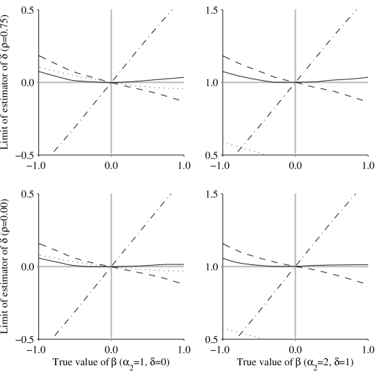
It may be observed that, when the true value of $\beta$ is 0, the limit $\delta_{*}$ is equal to true value of $\delta$ for both estimators $\hat{\delta}_{null}$ and $\hat{\delta}_{cov}$. This is in agreement with our conclusion above about the asymptotic behavior of the proposed estimator. When the true value of $\beta$ is different from 0, instead, this does not happen but, at least for $\hat{\delta}_{cov}$, the distance of $\delta_{*}$ from the true $\delta$ is surprisingly small and does not seem to be affected by the correlation between $U$ and $V$ which is measured by $\rho$. We recall that, although our estimator is derived under the assumption that $C$ is conditionally independent of $U$ given $V$, this result is obtained under a model which assumes that both $U$ and $V$ have a direct effect on $C$.

A final points concerns the ITT and TR estimators. The first is adequate only if the true value of $\delta$ is equal to 0 (plots on the left of Figure 1), whereas it is completely inadequate when it is equal to 1 (plots on the right). The TR estimator, instead, is consistent only when the true value of $\beta$ is equal to 0, but in the other cases it has a strong bias. Overall, even if based on a logistic regression method, these two estimators behave much worse than our estimator.

4.2.2 Finite-sample properties

In order to assess the finite-sample properties of the two-step estimator, we performed a simulation study based on 1000 samples of size $n=200,500$ generated from the model based on assumptions (14) and (15). For each simulated sample, we computed the estimators $\hat{\mbox{\boldmath$\alpha$}}=(\hat{\alpha}_{1},\hat{\alpha}_{2})^{\prime}$, $\hat{\beta}$ and $\hat{\delta}$ based of a model for the probability to comply of type (11), with $\mbox{\boldmath$m$}(v)=(1,v)^{\prime}$. Using the notation of Section 4.2.1, these estimators could also be denoted by $\hat{\mbox{\boldmath$\alpha$}}_{cov}$, $\hat{\beta}_{cov}$ and $\hat{\delta}_{cov}$. The results, in term of bias and standard deviation of the estimators and in terms of mean of the standard errors, are reported in Table 1 (when the true value of $\delta$ is 0) and in Table 2 (when the true value of $\delta$ is 1). Note that, for small sample sizes as those we are considering here, it may happen that there are not discordant configurations. Consequently, we apply the rule of thumb described in Section 4.1 to prevent instabilities of the estimator.

$n$ $\rho$ $\alpha_{1}$ $\alpha_{2}$ $\beta$ $\hat{\alpha}_{1}$ $\hat{\alpha}_{2}$ $\hat{\beta}$ $\hat{\delta}$
200 0.00 2 1 -1 bias 0.072 0.045 -0.144 0.117
st.dev. (0.606) (0.596) (1.344) (1.099)
mean s.e. (0.658) (0.573) (1.410) (1.097)
1 1 0 bias 0.078 0.070 -0.024 0.017
st.dev. (0.575) (0.622) (1.268) (1.041)
mean s.e. (0.555) (0.578) (1.222) (1.019)
0 1 1 bias 0.024 0.096 0.021 0.051
st.dev. (0.556) (0.614) (1.226) (1.037)
mean s.e. (0.553) (0.585) (1.204) (1.000)
200 0.75 2 1 -1 bias 0.122 0.098 -0.178 0.153
st.dev. (0.621) (0.632) (1.386) (1.171)
mean s.e. (0.658) (0.602) (1.380) (1.093)
1 1 0 bias 0.079 0.079 -0.084 0.084
st.dev. (0.564) (0.615) (1.184) (0.991)
mean s.e. (0.543) (0.592) (1.155) (0.985)
0 1 1 bias 0.038 0.111 -0.044 0.117
st.dev. (0.568) (0.601) (1.200) (0.995)
mean s.e. (0.547) (0.597) (1.132) (0.959)
500 0.00 2 1 -1 bias 0.058 0.048 -0.176 0.165
st.dev. (0.407) (0.356) (0.897) (0.678)
mean s.e. (0.399) (0.350) (0.853) (0.662)
1 1 0 bias 0.021 0.035 -0.004 0.018
st.dev. (0.354) (0.358) (0.787) (0.641)
mean s.e. (0.334) (0.348) (0.733) (0.609)
0 1 1 bias 0.010 0.047 -0.004 0.041
st.dev. (0.343) (0.351) (0.733) (0.604)
mean s.e. (0.333) (0.349) (0.711) (0.590)
500 0.75 2 1 -1 bias 0.055 0.011 -0.129 0.085
st.dev. (0.411) (0.366) (0.837) (0.647)
mean s.e. (0.387) (0.354) (0.799) (0.632)
1 1 0 bias 0.007 0.022 0.022 -0.007
st.dev. (0.329) (0.360) (0.700) (0.575)
mean s.e. (0.327) (0.353) (0.693) (0.589)
0 1 1 bias 0.019 0.023 -0.036 0.040
st.dev. (0.343) (0.370) (0.700) (0.581)
mean s.e. (0.333) (0.354) (0.686) (0.574)
Table 1: Simulation results for the proposed two-step estimator based on 1000 samples of size $n=500,1000$ generated under different models based on assumptions (14) and (15), with $\rho=0.00,0.75$ and different values of $\alpha_{1}$ and $\beta$ (in each case $\alpha_{2}=1$ and $\delta=0$).
$n$ $\rho$ $\alpha_{1}$ $\alpha_{2}$ $\beta$ $\hat{\alpha}_{1}$ $\hat{\alpha}_{2}$ $\hat{\beta}$ $\hat{\delta}$
200 0.00 2 2 -1 bias 0.049 0.077 -0.075 0.103
st.dev. (0.593) (0.620) (1.363) (1.135)
mean s.e. (0.648) (0.726) (1.403) (1.193)
1 2 0 bias 0.041 0.096 0.032 0.022
st.dev. (0.556) (0.646) (1.237) (1.066)
mean s.e. (0.550) (0.734) (1.212) (1.119)
0 2 1 bias 0.053 0.140 -0.052 0.140
st.dev. (0.556) (0.627) (1.190) (1.020)
mean s.e. (0.553) (0.741) (1.190) (1.097)
200 0.75 2 2 -1 bias 0.101 0.111 -0.165 0.175
st.dev. (0.610) (0.657) (1.330) (1.127)
mean s.e. (0.645) (0.745) (1.348) (1.171)
1 2 0 bias 0.064 0.112 -0.016 0.064
st.dev. (0.591) (0.645) (1.225) (1.044)
mean s.e. (0.548) (0.743) (1.168) (1.096)
0 2 1 bias 0.024 0.124 -0.013 0.114
st.dev. (0.575) (0.621) (1.162) (0.985)
mean s.e. (0.554) (0.749) (1.143) (1.068)
500 0.00 2 2 -1 bias 0.065 0.060 -0.175 0.170
st.dev. (0.434) (0.476) (0.904) (0.735)
mean s.e. (0.399) (0.445) (0.840) (0.710)
1 2 0 bias 0.030 0.077 -0.010 0.057
st.dev. (0.327) (0.445) (0.720) (0.671)
mean s.e. (0.334) (0.447) (0.731) (0.673)
0 2 1 bias 0.024 0.084 -0.015 0.075
st.dev. (0.342) (0.487) (0.742) (0.697)
mean s.e. (0.333) (0.451) (0.716) (0.662)
500 0.75 2 2 -1 bias 0.054 0.062 -0.134 0.142
st.dev. (0.413) (0.458) (0.832) (0.716)
mean s.e. (0.387) (0.451) (0.798) (0.693)
1 2 0 bias 0.024 0.067 -0.012 0.056
st.dev. (0.350) (0.474) (0.723) (0.685)
mean s.e. (0.330) (0.451) (0.698) (0.656)
0 2 1 bias 0.041 0.066 -0.064 0.088
st.dev. (0.336) (0.475) (0.701) (0.664)
mean s.e. (0.333) (0.451) (0.688) (0.642)
Table 2: Simulation results for the proposed two-step estimator based on 1000 samples of size $n=500,1000$ generated under different models based on assumptions (14) and (15), with $\rho=0.00,0.75$ and different values of $\alpha_{1}$ and $\beta$ (in each case $\alpha_{2}=2$ and $\delta=1$).

The simulations show that the estimators always have a very low bias which, as may expected, tends to be smaller when the true value of $\beta$ is equal to 0 and when $n=500$ instead of $n=200$. It is also worth noting that this bias is not considerably affected by $\rho$. These conclusions are in agreement with those regarding the asymptotic behavior of the estimator drawn on the basis of Figure 2. Consequently, the rule of thumb that we use when all the possible discordant configurations are not present seems to work properly.

For what concerns the variability of the estimators, we observe that the standard error of each of them is roughly proportional to $1/\sqrt{n}$. This property is also in agreement with the asymptotic results illustrated in Section 4.2.1. Finally, for each estimator, the average standard error is close enough to its standard deviation. Relevant differences are only observed for $n=200$ when the standard error occasionally tends to be larger than the standard deviation. This confirms the validity of the proposed estimator of the variance-covariance matrix of $\hat{\mbox{\boldmath$\theta$}}$ which is based on the sandwich formula given in (13).

5 Dealing with missing responses

We now illustrate how the proposed causal model and the two-step conditional logistic estimator may be extended to the case of missing responses. For this aim, we introduce the binary indicator $R_{h}$, $h=1,2$, equal to 1 if the response variable $Y_{h}$ is observable and to 0 otherwise.

5.1 Causal model

With missing responses, we extend the model introduced in Section 2 by assuming that:

  • B1:

    R1β€‹βŠ§β€‹Y1|(U,𝑽)conditionalsubscript𝑅1⊧subscriptπ‘Œ1π‘ˆπ‘½R_{1}\>\begin{sideways}$\models$\end{sideways}\>Y_{1}|(U,\mbox{\boldmath$V$});

  • B2:

    Cβ€‹βŠ§β€‹(R1,Y1)|(U,𝑽)conditional𝐢⊧subscript𝑅1subscriptπ‘Œ1π‘ˆπ‘½C\>\begin{sideways}$\models$\end{sideways}\>(R_{1},Y_{1})|(U,\mbox{\boldmath$V$});

  • B3:

    Zβ€‹βŠ§β€‹(U,Y1,R1,C)|𝑽conditionalπ‘βŠ§π‘ˆsubscriptπ‘Œ1subscript𝑅1𝐢𝑽Z\>\begin{sideways}$\models$\end{sideways}\>(U,Y_{1},R_{1},C)|\mbox{\boldmath$V$};

  • B4:

    Xβ€‹βŠ§β€‹(U,𝑽,Y1,R1)|(C,Z)conditionalπ‘‹βŠ§π‘ˆπ‘½subscriptπ‘Œ1subscript𝑅1𝐢𝑍X\>\begin{sideways}$\models$\end{sideways}\>(U,\mbox{\boldmath$V$},Y_{1},R_{1})|(C,Z) and, with probability 1, X=Z𝑋𝑍X=Z when C=1𝐢1C=1 (compliers) and X=0𝑋0X=0 when C=0𝐢0C=0 (never-takers);

  • B5:

    Y2β€‹βŠ§β€‹(Y1,R1,Z)|(U,𝑽,C,X)conditionalsubscriptπ‘Œ2⊧subscriptπ‘Œ1subscript𝑅1π‘π‘ˆπ‘½πΆπ‘‹Y_{2}\>\begin{sideways}$\models$\end{sideways}\>(Y_{1},R_{1},Z)|(U,\mbox{\boldmath$V$},C,X);

  • B6:

    R2β€‹βŠ§β€‹(Y1,R1,Z,Y2)|(U,𝑽,C,X)conditionalsubscript𝑅2⊧subscriptπ‘Œ1subscript𝑅1𝑍subscriptπ‘Œ2π‘ˆπ‘½πΆπ‘‹R_{2}\>\begin{sideways}$\models$\end{sideways}\>(Y_{1},R_{1},Z,Y_{2})|(U,\mbox{\boldmath$V$},C,X);

  • B7:

    for any $u,\mbox{\boldmath$v$},c$ and $x$, we have

    $${\rm logit}[p(Y_{2}=1|u,\mbox{\boldmath$v$},c,x)]-{\rm logit}[p(Y_{1}=1|u,\mbox{\boldmath$v$})]=\mbox{\boldmath$a$}(\mbox{\boldmath$v$},x)^{\prime}\mbox{\boldmath$\alpha$}+c(1-x)\mbox{\boldmath$b$}(\mbox{\boldmath$v$})^{\prime}\mbox{\boldmath$\beta$},$$

    with the functions $\mbox{\boldmath$a$}(\mbox{\boldmath$v$},x)$ and $\mbox{\boldmath$b$}(\mbox{\boldmath$v$})$ and the corresponding parameter vectors defined as in Section 2.1.

New assumptions are essentially B1 and B6 concerning the conditional independence between $R_{1}$ and $Y_{1}$ and that between $R_{2}$ and $Y_{2}$ given observable and unobservable covariates. This assumption is weaker than the assumption that responses are missing at random given the observable covariates [20].

The resulting model is represented by the DAG in Figure 3.

Refer to caption
Figure 3: DAG for the model based on assumptions B1-B7. $U$ and $V$ represent unobservable and observable covariates affecting the response variables $Y_{1}$ and $Y_{2}$ and the indicator variables $R_{1}$ and $R_{2}$ for the response variables being observable, $C$ is a binary variable for the compliance status and $Z$ and $X$ are binary variables for the assigned and the received treatment.

5.2 Two-step conditional logistic estimator

Under assumptions B1-B7, we have that

$$p(y_{1},r_{1},z,x,y_{2},r_{2}|u,\mbox{\boldmath$v$},c)=p(y_{1}|u,\mbox{\boldmath$v$})p(r_{1}|u,\mbox{\boldmath$v$})p(z|\mbox{\boldmath$v$})p(x|c,z)p(y_{2}|u,\mbox{\boldmath$v$},c,x)p(r_{2}|u,\mbox{\boldmath$v$},c,x).$$

Then, marginalizing with respect to $C$ and $U$, we find that the probability mass function of the conditional distribution of $(Y_{1},R_{1},Z,X,Y_{2},R_{2})$ given $V$ is equal to

$\displaystyle f^{*}(y_{1},r_{1},z,x,y_{2},r_{2}|\mbox{\boldmath$v$})$ $\displaystyle=$ $\displaystyle p(z|\mbox{\boldmath$v$})\int\frac{e^{y_{+}\lambda(u,\mbox{\footnotesize\boldmath{$v$}})}}{1+e^{\lambda(u,\mbox{\footnotesize\boldmath{$v$}})}}p(r_{1}|u,\mbox{\boldmath$v$})\times$
$\displaystyle\times$ $\displaystyle\sum_{c}p(x|c,z)\frac{e^{y_{2}t(c,\mbox{\footnotesize\boldmath{$v$}},x)}}{1+e^{\lambda(u,\mbox{\footnotesize\boldmath{$v$}})+t(c,\mbox{\footnotesize\boldmath{$v$}},x)}}p(r_{2}|u,\mbox{\boldmath$v$},c,x)\pi(c|u,\mbox{\boldmath$v$})\phi(u|\mbox{\boldmath$v$})du,$

where, as in Section 3, $t(c,\mbox{\boldmath$v$},x)=\mbox{\boldmath$a$}(\mbox{\boldmath$v$},x)^{\prime}\mbox{\boldmath$\alpha$}+c(1-x)\mbox{\boldmath$b$}(\mbox{\boldmath$v$})^{\prime}\mbox{\boldmath$\beta$}$.

When $z=1$, the above expression simplifies to

$\displaystyle f^{*}(y_{1},r_{1},1,x,y_{2},r_{2}|\mbox{\boldmath$v$})$ $\displaystyle=$ $\displaystyle p(Z=1|\mbox{\boldmath$v$})\times$
$\displaystyle\times$ $\displaystyle\int\frac{e^{y_{+}\lambda(u,\mbox{\footnotesize\boldmath{$v$}})}}{1+e^{\lambda(u,\mbox{\footnotesize\boldmath{$v$}})}}p(r_{1}|u,\mbox{\boldmath$v$})\frac{e^{y_{2}\mbox{\footnotesize\boldmath{$a$}}(\mbox{\footnotesize\boldmath{$v$}},x)^{\prime}\mbox{\footnotesize\boldmath{$\alpha$}}}}{1+e^{\lambda(u,\mbox{\footnotesize\boldmath{$v$}})+\mbox{\footnotesize\boldmath{$a$}}(\mbox{\footnotesize\boldmath{$v$}},x)^{\prime}\mbox{\footnotesize\boldmath{$\alpha$}}}}p(r_{2}|u,\mbox{\boldmath$v$},c,x)\phi(u|\mbox{\boldmath$v$})du,$

and this implies that

$$f^{*}(y_{2}|\mbox{\boldmath$v$},1,x)=\frac{f^{*}(1-y_{2},1,1,x,y_{2},1|\mbox{\boldmath$v$})}{f^{*}(0,1,1,x,1,1|\mbox{\boldmath$v$})+f^{*}(1,1,1,x,0,1|\mbox{\boldmath$v$})}=\frac{e^{y_{2}\mbox{\footnotesize\boldmath{$a$}}(\mbox{\footnotesize\boldmath{$v$}},x)^{\prime}\mbox{\footnotesize\boldmath{$\alpha$}}}}{1+e^{\mbox{\footnotesize\boldmath{$a$}}(\mbox{\footnotesize\boldmath{$v$}},x)^{\prime}\mbox{\footnotesize\boldmath{$\alpha$}}}},$$

where, in general, $f^{*}(y_{2}|\mbox{\boldmath$v$},z,x)=p(y_{2}|\mbox{\boldmath$v$},R_{1}=1,z,x,R_{2}=1,Y_{+}=1)$. This is due to the definition of $p(x|c,z)$ which, as already noted, may only be equal to 0 or 1. The same does not happen when $z=0$ since in this case

$\displaystyle f^{*}(y_{1},r_{1},0,0,y_{2},r_{2}|\mbox{\boldmath$v$})$ $\displaystyle=$ $\displaystyle p(Z=0|\mbox{\boldmath$v$})g^{*}(y_{1},r_{1},y_{2},r_{2}|bv)$
$\displaystyle g^{*}(y_{1},r_{1},y_{2},r_{2}|\mbox{\boldmath$v$})$ $\displaystyle=$ $\displaystyle\int\frac{e^{y_{+}\lambda(u,\mbox{\footnotesize\boldmath{$v$}})}}{1+e^{\lambda(u,\mbox{\footnotesize\boldmath{$v$}})}}p(r_{1}|u,\mbox{\boldmath$v$})\times$
$\displaystyle\times$ $\displaystyle\sum_{c}\frac{e^{y_{2}t(c,\mbox{\footnotesize\boldmath{$v$}},0)}}{1+e^{\lambda(u,\mbox{\footnotesize\boldmath{$v$}})+t(c,\mbox{\footnotesize\boldmath{$v$}},0)}}p(r_{2}|u,\mbox{\boldmath$v$},c,0)\pi(c|u,\mbox{\boldmath$v$})\phi(u|\mbox{\boldmath$v$})du.$

Then, as in Section 4, we consider a first-order Taylor series expansion of $\log g^{*}(y_{1},r_{1},y_{2},r_{2}|\mbox{\boldmath$v$})$ around $\mbox{\boldmath$\beta$}=\mbox{\boldmath$0$}$ and we find that

$$\log g^{*}(y_{1},r_{1},y_{2},r_{2}|\mbox{\boldmath$v$})\approx\log g^{*}_{0}(y_{1},r_{1},y_{2},r_{2}|\mbox{\boldmath$v$})+h^{*}(y_{1},r_{1},y_{2},r_{2}|\mbox{\boldmath$v$})\mbox{\boldmath$b$}(\mbox{\boldmath$v$})^{\prime}\mbox{\boldmath$\beta$}$$

where $g_{0}^{*}(y_{1},r_{1},y_{2},r_{2}|\mbox{\boldmath$v$})$ is the function $g^{*}(y_{1},r_{1},y_{2},r_{2}|\mbox{\boldmath$v$})$ computed at $\mbox{\boldmath$\beta$}=\mbox{\boldmath$0$}$ and

$\displaystyle h^{*}(y_{1},r_{1},y_{2},r_{2}|\mbox{\boldmath$v$})$ $\displaystyle=$ $\displaystyle\frac{2y_{2}-1}{g_{0}^{*}(y_{1},r_{1},y_{2},r_{2}|\mbox{\boldmath$v$})}\int\frac{e^{y_{+}\lambda(u,\mbox{\footnotesize\boldmath{$v$}})}}{1+e^{\lambda(u,\mbox{\footnotesize\boldmath{$v$}})}}p(r_{1}|u,\mbox{\boldmath$v$})\times$
$\displaystyle\times$ $\displaystyle\frac{e^{t(0,\mbox{\footnotesize\boldmath{$v$}},0)}}{[1+e^{\lambda(u,\mbox{\footnotesize\boldmath{$v$}})+t(0,\mbox{\footnotesize\boldmath{$v$}},0)}]^{2}}p(r_{2}|u,\mbox{\boldmath$v$},c,0)\pi(1|u,\mbox{\boldmath$v$})\phi(u|\mbox{\boldmath$v$})du.$

Consequently, we have

$$\log\frac{f^{*}(0,1,0,0,1,1|\mbox{\boldmath$v$})}{f^{*}(1,1,0,0,0,1|\mbox{\boldmath$v$})}\approx\mbox{\boldmath$a$}(\mbox{\boldmath$v$},0)^{\prime}\mbox{\boldmath$\alpha$}+h^{*}(\mbox{\boldmath$v$})\mbox{\boldmath$b$}(\mbox{\boldmath$v$})^{\prime}\mbox{\boldmath$\beta$},$$

where $h^{*}(\mbox{\boldmath$v$})$ is a correction factor which is simply equal to $\pi(1|\mbox{\boldmath$v$})=p(C=1|\mbox{\boldmath$v$})$ when $C$ is conditionally independent of $U$ given $V$. Finally, we have

$$f^{*}(y_{2}|\mbox{\boldmath$v$},0,0)\approx\frac{e^{\mbox{\footnotesize\boldmath{$a$}}(\mbox{\footnotesize\boldmath{$v$}},0)^{\prime}\mbox{\footnotesize\boldmath{$\alpha$}}+h(\mbox{\footnotesize\boldmath{$v$}})\mbox{\footnotesize\boldmath{$b$}}(\mbox{\footnotesize\boldmath{$v$}})^{\prime}\mbox{\footnotesize\boldmath{$\beta$}}}}{1+e^{\mbox{\footnotesize\boldmath{$a$}}(\mbox{\footnotesize\boldmath{$v$}},0)^{\prime}\mbox{\footnotesize\boldmath{$\alpha$}}+h(\mbox{\footnotesize\boldmath{$v$}})\mbox{\footnotesize\boldmath{$b$}}(\mbox{\footnotesize\boldmath{$v$}})^{\prime}\mbox{\footnotesize\boldmath{$\beta$}}}},$$

which is exactly the same expression given in (10).

On the basis of the above arguments, in the case of missing responses we propose to use a two-step estimator which has the same structure as that described in Section 4.1 and is based on a logit model of type (11) for the probability $\pi(1|\mbox{\boldmath$v$})$ of being a complier given the covariates. Here, for each subject $i$, with $i=1,\ldots,n$, we observe $\mbox{\boldmath$v$}_{i}$, $r_{i1}$, $z_{i}$, $x_{i}$ and $r_{i2}$, where, for $h=1,2$, $r_{hi}$ is the observed value of $R_{h}$. For the same subject we also observe $y_{i1}$ if $r_{i1}=1$ and $y_{i2}$ if $r_{i2}=1$.

The estimator is based on the following steps which, as for the initial estimator, may be performed on the basis of standard estimation algorithms:

  1. 1.

    Estimation of $\eta$. This is based on the observed values $\mbox{\boldmath$v$}_{i}$ and $x_{i}$ for every $i$ such that $z_{i}=1$ and proceeds by maximizing the weighted log-likelihood

    $$\ell_{1}^{*}(\mbox{\boldmath$\eta$})=\sum_{i}\frac{z_{i}}{p(z_{i}|\mbox{\boldmath$v$}_{i})}[x_{i}\log\pi(1|\mbox{\boldmath$v$}_{i})+(1-x_{i})\log\pi(0|\mbox{\boldmath$v$}_{i})].$$
  2. 2.

    Estimation of $\alpha$ and $\beta$. This is performed by maximizing the conditional log-likelihood

    $$\ell_{2}(\mbox{\boldmath$\alpha$},\mbox{\boldmath$\beta$};\mbox{\boldmath$\eta$})=\sum_{i}d_{i}r_{i1}r_{i2}\ell_{i2}(\mbox{\boldmath$\alpha$},\mbox{\boldmath$\beta$};\mbox{\boldmath$\eta$}),$$

    where $\ell_{i2}(\mbox{\boldmath$\alpha$},\mbox{\boldmath$\beta$};\mbox{\boldmath$\eta$})$ is defined as in (12).

Note that the only difference with respect to the estimator in Section 4.1 is in the second step where we consider only the subjects who respond at both occasions, whereas at the first step we consider all subjects in order to estimate the model for the probability of being a complier. Moreover, standard errors for the estimator can again be computed on the basis of the sandwich formula (13).

5.3 Properties of the two-step estimator

A final point concerns the properties of the estimators 𝜢^^𝜢\hat{\mbox{\boldmath$\alpha$}}, 𝜷^^𝜷\hat{\mbox{\boldmath$\beta$}} and Ξ΄^​(𝒗)^𝛿𝒗\hat{\delta}(\mbox{\boldmath$v$}) with missing responses. These estimators have the same asymptotic properties they have when the response variables are always observable (see Section 4.2.1). The main result is that these estimators are consistent when 𝜷0=𝟎subscript𝜷00\mbox{\boldmath$\beta$}_{0}=\mbox{\boldmath$0$}, regardless of the parametrization used in the logit model (11) for the probability to comply. When 𝜷0β‰ πŸŽsubscript𝜷00\mbox{\boldmath$\beta$}_{0}\neq\mbox{\boldmath$0$}, the estimators 𝜢^^𝜢\hat{\mbox{\boldmath$\alpha$}} and 𝜷^^𝜷\hat{\mbox{\boldmath$\beta$}} converge to πœΆβˆ—subscript𝜢\mbox{\boldmath$\alpha$}_{*} and πœ·βˆ—subscript𝜷\mbox{\boldmath$\beta$}_{*}, respectively, as nβ†’βˆžβ†’π‘›n\rightarrow\infty. These limits are equal to the true values 𝜢0subscript𝜢0\mbox{\boldmath$\alpha$}_{0} and 𝜷0subscript𝜷0\mbox{\boldmath$\beta$}_{0} when 𝜷0=𝟎subscript𝜷00\mbox{\boldmath$\beta$}_{0}=\mbox{\boldmath$0$} and are expected to be reasonably close to these true values when 𝜷0subscript𝜷0\mbox{\boldmath$\beta$}_{0} is not too far from 𝟎0. The same may be said for the estimator Ξ΄^​(𝒗)^𝛿𝒗\hat{\delta}(\mbox{\boldmath$v$}) which converges to Ξ΄βˆ—β€‹(𝒗)subscript𝛿𝒗\delta_{*}(\mbox{\boldmath$v$}).

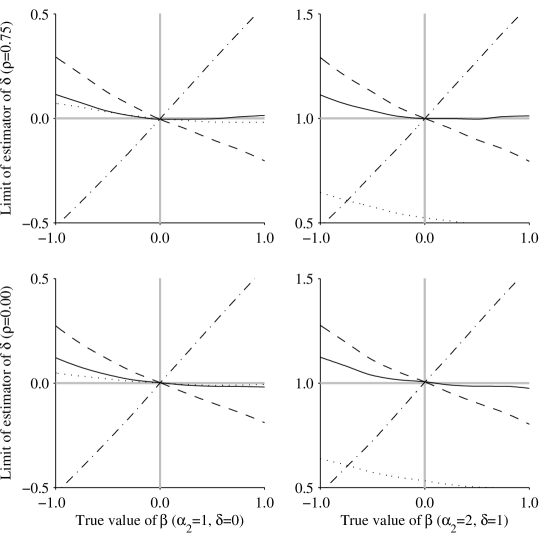
To illustrate the above point, in Figure 3 we report some plots of $\delta_{*}$ with respect to $\beta$ under a true model involving only one observable covariate and based on the same assumptions illustrated in Section 4.2.1, see in particular (14) and (15), beyond the assumption that $R_{1}$ and $R_{2}$ have Bernoulli distribution with probabilities of success chosen, respectively, as follows

$$\begin{array}[]{rcl}p(R_{1}=1|u,v)&=&{\rm expit}[1+(u+v)/\sqrt{1+\rho}/2],\vspace*{0.25cm}\\ p(R_{2}=1|u,v,c,x)&=&{\rm expit}[1+(u+v)/\sqrt{1+\rho}/2+c/2+x/2].\end{array}$$ (16)

The estimators we considered are:

  • β€’

    Ξ΄^n​u​l​lsubscript^𝛿𝑛𝑒𝑙𝑙\hat{\delta}_{null}: two-step conditional logistic estimator of $\delta$ based on a model for the probability to comply of type (11) with $m(v)=1$;

  • β€’

    Ξ΄^c​o​vsubscript^π›Ώπ‘π‘œπ‘£\hat{\delta}_{cov}: as above with $\mbox{\boldmath$m$}(v)=(1,v)^{\prime}$, so that the covariate is also used to predict the probability to comply;

  • β€’

    Ξ΄^i​t​tsubscript^𝛿𝑖𝑑𝑑\hat{\delta}_{itt}: ITT estimator based on the conditional logistic regression on only the subjects who respond at both occasions, i.e. we regress $Y_{2}$ on $(1,Z)$ given $Y_{+}=1$, $R_{1}=1$ and $R_{2}=1$;

  • β€’

    Ξ΄^t​rsubscript^π›Ώπ‘‘π‘Ÿ\hat{\delta}_{tr}: TR estimator based the conditional logistic regression of $Y_{2}$ on $(1,X)$ given $Y_{+}=1$, $R_{1}=1$ and $R_{2}=1$.

The resulting plots closely resemble those in Figure 2 and then similar conclusions may be drawn about the proposed estimator. In particular, we again note the small distance between the limit in probability of the estimator and the true value of the parameter.

Refer to caption
Figure 4: Limit of the estimators $\hat{\delta}_{null}$ (dashed line), $\hat{\delta}_{cov}$ (solid line), $\hat{\delta}_{itt}$ (dotted line) and $\hat{\delta}_{tr}$ (dash-dotted line) under assumptions (14), (15) and (16), with $\rho=0.00,0.75$, $\beta$ between -1 and 1 and $\delta=0,1$, with $\alpha_{1}$ and $\alpha_{2}$ defined accordingly.

Under the same true model assumed above, we studied by simulation the finite-sample properties of the estimators $\hat{\mbox{\boldmath$\alpha$}}$, $\hat{\mbox{\boldmath$\beta$}}$ and $\hat{\delta}$. As usual, we focused on the estimators which exploit the covariate to predict the probability to comply, and then we let $\mbox{\boldmath$m$}(\mbox{\boldmath$v$})=(1,v)^{\prime}$ in (11). Under the same setting of the simulations in Section 4.2.2, we obtained the results reported in Tables 3 and 4 when (16) is assumed. These results are very similar to those reported in Tables 1 and 2 for the case in which the response variables are always observed. The main difference is in the variability of the estimators which is obviously larger because of the presence of missing responses.

$n$ $\rho$ $\alpha_{1}$ $\alpha_{2}$ $\beta$ $\hat{\alpha}_{1}$ $\hat{\alpha}_{2}$ $\hat{\beta}$ $\hat{\delta}$
200 0.00 2 1 -1 bias -0.107 0.076 0.208 -0.025
st.dev. (0.628) (0.706) (1.573) (1.404)
mean s.e. (0.910) (0.733) (1.910) (1.445)
1 1 0 bias 0.053 0.129 0.024 0.053
st.dev. (0.710) (0.723) (1.624) (1.369)
mean s.e. (0.825) (0.742) (1.736) (1.356)
0 1 1 bias 0.045 0.071 0.061 -0.034
st.dev. (0.776) (0.683) (1.654) (1.310)
mean s.e. (0.813) (0.725) (1.686) (1.303)
200 0.75 2 1 -1 bias -0.069 0.065 0.161 -0.028
st.dev. (0.639) (0.696) (1.457) (1.310)
mean s.e. (0.928) (0.752) (1.841) (1.381)
1 1 0 bias 0.078 0.069 -0.035 0.026
st.dev. (0.720) (0.699) (1.515) (1.213)
mean s.e. (0.813) (0.751) (1.625) (1.283)
0 1 1 bias 0.003 0.076 0.067 0.007
st.dev. (0.801) (0.696) (1.613) (1.256)
mean s.e. (0.816) (0.750) (1.575) (1.228)
500 0.00 2 1 -1 bias 0.113 0.070 -0.272 0.230
st.dev. (0.594) (0.467) (1.235) (0.907)
mean s.e. (0.608) (0.440) (1.211) (0.862)
1 1 0 bias 0.023 0.038 -0.008 0.023
st.dev. (0.512) (0.457) (1.022) (0.809)
mean s.e. (0.482) (0.438) (0.998) (0.781)
0 1 1 bias 0.036 0.008 0.028 -0.056
st.dev. (0.482) (0.443) (1.009) (0.785)
mean s.e. (0.476) (0.433) (0.976) (0.759)
500 0.75 2 1 -1 bias 0.088 0.037 -0.187 0.135
st.dev. (0.578) (0.463) (1.123) (0.844)
mean s.e. (0.596) (0.451) (1.142) (0.823)
1 1 0 bias 0.042 0.064 -0.025 0.047
st.dev. (0.530) (0.468) (1.045) (0.799)
mean s.e. (0.490) (0.454) (0.964) (0.758)
0 1 1 bias 0.035 0.035 0.001 -0.001
st.dev. (0.503) (0.482) (0.976) (0.769)
mean s.e. (0.483) (0.454) (0.937) (0.735)
Table 3: Simulation results for the proposed two-step estimator based on 1000 samples of size $n=500,1000$ generated under different models based on assumptions (14) and (15) and (16), with $\rho=0.00,0.75$ and different values of $\alpha_{1}$ and $\beta$ (in each case $\alpha_{2}=1$ and $\delta=0$).
$n$ $\rho$ $\alpha_{1}$ $\alpha_{2}$ $\beta$ $\hat{\alpha}_{1}$ $\hat{\alpha}_{2}$ $\hat{\beta}$ $\hat{\delta}$
200 0.00 2 2 -1 bias -0.084 -0.019 0.227 -0.162
st.dev. (0.590) (0.614) (1.547) (1.329)
mean s.e. (0.913) (0.876) (1.915) (1.531)
1 2 0 bias 0.056 0.010 -0.046 0.000
st.dev. (0.733) (0.614) (1.644) (1.307)
mean s.e. (0.818) (0.879) (1.713) (1.426)
0 2 1 bias 0.043 -0.021 0.070 -0.134
st.dev. (0.784) (0.589) (1.650) (1.236)
mean s.e. (0.815) (0.871) (1.686) (1.389)
200 0.75 2 2 -1 bias -0.092 -0.022 0.188 -0.118
st.dev. (0.617) (0.604) (1.436) (1.239)
mean s.e. (0.912) (0.890) (1.827) (1.468)
1 2 0 bias 0.033 -0.014 0.101 -0.148
st.dev. (0.714) (0.607) (1.513) (1.198)
mean s.e. (0.799) (0.892) (1.595) (1.364)
0 2 1 bias 0.031 -0.037 0.021 -0.089
st.dev. (0.801) (0.591) (1.549) (1.137)
mean s.e. (0.819) (0.880) (1.593) (1.322)
500 0.00 2 2 -1 bias 0.071 0.129 -0.186 0.243
st.dev. (0.601) (0.602) (1.256) (1.005)
mean s.e. (0.599) (0.587) (1.202) (0.954)
1 2 0 bias 0.065 0.115 -0.073 0.122
st.dev. (0.505) (0.598) (1.029) (0.883)
mean s.e. (0.490) (0.582) (1.012) (0.881)
0 2 1 bias 0.023 0.138 0.049 0.066
st.dev. (0.494) (0.583) (0.995) (0.875)
mean s.e. (0.475) (0.586) (0.978) (0.863)
500 0.75 2 2 -1 bias 0.112 0.123 -0.263 0.274
st.dev. (0.583) (0.586) (1.148) (0.933)
mean s.e. (0.598) (0.594) (1.140) (0.912)
1 2 0 bias 0.034 0.098 -0.033 0.097
st.dev. (0.507) (0.588) (1.009) (0.848)
mean s.e. (0.484) (0.591) (0.952) (0.849)
0 2 1 bias 0.060 0.130 -0.085 0.155
st.dev. (0.476) (0.612) (0.917) (0.827)
mean s.e. (0.477) (0.601) (0.920) (0.832)
Table 4: Simulation results for the proposed two-step estimator based on 1000 samples of size $n=500,1000$ generated under different models based on assumptions (14) and (15) and (16), with $\rho=0.00,0.75$ and different values of $\alpha_{1}$ and $\beta$ (in each case $\alpha_{2}=2$ and $\delta=1$).

6 An application

To illustrate the approach proposed in this paper, we analyzed the dataset coming from the randomized experiment on BSE already mentioned in Section 1.

The study took place between the beginning of 1988 and the end of 1990 at the Oncologic Center of the Faenza District, Italy. The sample used in the study consists of 657 women aged 20 to 64 years, who were randomly assigned to the control, consisting of learning how to perform BSE through a standard method, or to the treatment, consisting of a training course held by a specialized medical staff. Only women assigned to the treatment can access it and then non-compliance may be observed only among these subjects. In particular, of the 330 women randomly assigned to the treatment, 182 attended the course and so they may be considered as compliers; the remaining women may be considered as never-takes.

The efficacy of the treatment is measured by two binary response variables, observed before and after the treatment/control, which indicate if BSE is regularly practised and if the quality of BSE practise is adequate. Several covariates are also available, such as age, number of children, educational level, occupational status, presence of previous cancer pathologies in the woman or her family, menopause and adequate knowledge of breast pathophysiology. Finally, some response variables are not observed and these have to be treated as missing.

The dataset has already been analyzed by [5], on the basis of a standard conditional logistic approach, and by [6], who exploited a potential outcome approach allowing for missing responses, which is related to that of [21].

In analyzing the dataset, we first considered the effect of the treatment on practicing BSE. In this case, $Y_{1}$ is equal to 1 if a woman regularly practises BSE before the treatment and to 0 otherwise. Similarly, $Y_{2}$ is equal to 1 if a woman regularly practises BSE after the treatment and to 0 otherwise. The first variable was observed for the 93.61% of the sample and the second for the 65.30%. We then followed the method for missing responses described in Section 5 under assumption (2) for the parametrization of the causal model. In particular, we first computed the estimators $\hat{\mbox{\boldmath$\alpha$}}_{null}$, $\hat{\beta}_{null}$ and $\hat{\delta}_{null}$, based on predicting the probability to comply only on the basis of the indicator variable for the second response variable being observable, and the estimators $\hat{\mbox{\boldmath$\alpha$}}_{cov}$, $\hat{\beta}_{cov}$ and $\hat{\delta}_{cov}$, which also consider the covariates age and age-squared in the model used to predict this probability. These covariates are included since are among those with the most significant effect on the probability to comply. We also considered the ITT estimator $\hat{\delta}_{itt}$ and the TR estimator $\hat{\delta}_{tr}$ defined as in Section 5.3. The results are displayed in Table 5.

Our first conclusion is that the inclusion of the covariates in the model for the probability to comply does not dramatically affect the estimates of the parameters and of the causal effect computed following our approach. In particular, the estimate of $\alpha_{2}$ remains unchanged by the inclusion of these covariates, since this estimate exploits only the data deriving from the treatment arm. Overall, we can observe an effect of the control on never-takers, corresponding to $\alpha_{1}$, which is not significant. Moreover, the estimate of the parameter $\beta$ is very different from zero, indicating a great difference between compliers and never-takers for what concerns this effect. Then, we conclude that the effect of the treatment over control on practicing BSE ($\delta$) is not significant. A similar conclusion is reached on the basis of the ITT estimator of $\delta$, whereas the TR estimator attains a value much higher of that of the other estimators, since it does not distinguish between compliers and never-takers for what concerns the effect of the treatment.

$\hat{\mbox{\boldmath$\alpha$}}_{null}$ $\hat{\mbox{\boldmath$\alpha$}}_{cov}$
est. se $t$ $p$-value est. se $t$ $p$-value
-0.336 0.586 -0.575 0.566 -0.143 0.573 -0.250 0.802
2.241 0.470 4.763 0.000 2.241 0.471 4.763 0.000
$\hat{\beta}_{null}$ $\hat{\beta}_{cov}$
est. se $t$ $p$-value est. se $t$ $p$-value
2.779 1.207 2.302 0.021 2.382 1.244 1.914 0.056
$\hat{\delta}_{null}$ $\hat{\delta}_{cov}$
est. se $t$ $p$-value est. se $t$ $p$-value
-0.202 0.882 -0.229 0.819 0.002 0.909 0.003 0.998
$\hat{\delta}_{itt}$ $\hat{\delta}_{tr}$
est. se $t$ $p$-value est. se $t$ $p$-value
0.2701 0.4503 0.5998 0.5486 1.3652 0.5405 2.5260 0.0115
Table 5: Estimates of the causal parameters obtained on the basis of the proposed approach and the ITT and TR approaches when the response variable is equal to 1 for a woman regularly practicing BSE and to 0 otherwise.

We then considered the effect of the treatment on the quality of the BSE practise. As in [Mealli:2002], this is measured through the binary response variables $Y_{1}$ and $Y_{2}$ (here redefined) which are equal to 1 if the score assigned by the medical staff to the quality of the BSE practise is greater than the sample median and to 0 otherwise. As usual, $Y_{1}$ is a pre-treatment variable and $Y_{2}$ is a post-treatment variable. Obviously, these variables are observable only if BSE is practised and so we again used the method for missing responses described in Section 5. In particular, $Y_{1}$ was observed for the 54.80% of the sample and $Y_{2}$ for the 51.93%. The results obtained from the application of the same estimators mentioned above are reported in Table 6.

In this case, the inclusion of the covariates age and age-squared in the model for predicting the probability to comply has a slight effect on the estimates of the parameters $\alpha$, $\beta$ and $\delta$ computed on the basis of the proposed approach. Never-takers and compliers now appear to be less distant in terms of reaction to the control, whose effect is not significant for both subpopulations. On the other hand, the effect of the treatment on compliers is significant as well as the causal effect of the treatment over control. The estimate of this causal effect is in this case close to the RT estimate, whereas the ITT estimate is much smaller, even if it remains significantly greater than 0.

$\hat{\mbox{\boldmath$\alpha$}}_{null}$ $\hat{\mbox{\boldmath$\alpha$}}_{cov}$
est. se $t$ $p$-value est. se $t$ $p$-value
0.000 0.707 0.000 1.000 -0.112 0.687 -0.164 0.870
3.611 1.013 3.563 0.000 3.611 1.013 3.563 0.000
$\hat{\beta}_{null}$ $\hat{\beta}_{cov}$
est. se $t$ $p$-value est. se $t$ $p$-value
0.880 1.406 0.626 0.531 1.103 1.323 0.834 0.404
$\hat{\delta}_{null}$ $\hat{\delta}_{cov}$
est. se $t$ $p$-value est. se $t$ $p$-value
2.731 1.300 2.100 0.036 2.620 1.262 2.076 0.038
$\hat{\delta}_{itt}$ $\hat{\delta}_{tr}$
est. se $t$ $p$-value est. se $t$ $p$-value
1.6186 0.5704 2.8377 0.0045 3.2055 1.0537 3.0420 0.0024
Table 6: Estimates of the causal parameters obtained on the basis of the proposed approach and the ITT and TR approaches when the response variable is equal to 1 when the quality of the BSE practise is adequate and to 0 otherwise.

Overall, the results obtained with the proposed approach are in accordance with those of [5] and [6], who concluded that the training course has not a significant effect on practising BSE, but it has a significant effect on the quality of the BSE practise.

7 Discussion

A causal model has been introduced to study the behavior of the conditional logistic estimator as a tool of analysis of data coming from two-arm experimental studies with possible non-compliance. The model is applicable with binary outcomes observed before and after the treatment (or control). It is formulated on the basis of latent variables for the effect of unobservable covariates at both occasions and to account for the difference between compliers and never-takers in terms of reaction to control and treatment. A correction for the bias of the conditional logistic estimator has also been proposed which can be exploited when we want to estimate the causal effect of the treatment over control in the subpopulation of compliers. It results a two-step estimator which has some connection with the estimators of [14] and [15] and represents an extension of the standard conditional logistic estimator for this type of experiments. This estimator may be simply computed through standard algorithms for logistic regression and does not require to formulate assumptions on the distribution of the latent variables given the covariates. It also has interesting asymptotic and finite-sample properties which are maintained even with missing responses.

One of the basic assumptions on which the approach relies is that a subject is assigned to the control arm or to the treatment arm with a probability depending only on the observable covariates and not on the pre-treatment response variable. Indeed, we could relax this assumption, but we would have more complex expressions for the conditional probability of the response variables given their sum. Similarly, the approach can be extended to the case in which subjects assigned to both arm can access the treatment and then non-compliance may also exist in the control arm, i.e. certain subjects assigned to the control may decide instead to take the treatment. The model presented in Section 2 can be easily extended to this case. Using the terminology of [7], we have to consider the subpopulations of compliers, never-takers and always-takers. By exploiting an approximation similar to that illustrated in Section 3, we can set up an estimator of the causal effect of the treatment also in this case. The causal effect is again referred to the subpopulation of compliers and is measured on the logit scale. The approach would be complicated by the fact that the true model involves a mixture on three subpopulations. Moreover, the effect of the control on never-takers and that of the treatment on compliers is not directly observable from the treatment arm as it was in the original model. However, the resulting estimator would maintain its simplicity as main advantage, being based on a series of logistic regressions with suitable design matrices, which can be performed by standard algorithms.

As a final comment consider that, driven by the application on the BSE dataset, we only considered the case of repeated binary response variables. However, the approach may be easily extended to the case of response variables having a different nature (e.g. counting), provided that the conditional distribution of these variables belongs to the natural exponential family and the causal effect is measured on a scale defined according to the canonical link function for the adopted distribution [22].

Acknowledgements

I thank Dr. S. Ferro (Direzione Generale SanitΓ  e Politiche Sociali, Regione Emilia Romagna, IT) for providing the dataset on breast self examination and Dr. L. Grilli (University of Florence, IT) for interesting discussions on the approach. I acknowledge the financial support from Ministero dell’Istruzione, dell’UniversitΓ  e della Ricerca (PRIN 2005 - β€œModelli marginali per variabili categoriche con applicazioni all’analisi causale”).

Appendix

A1: Mathematical details on the approximation

In order to derive (8) consider that

$$\log g(1,0|\mbox{\boldmath$v$})-\log g(0,1|\mbox{\boldmath$v$})\approx\log g_{0}(1,0|\mbox{\boldmath$v$})-\log g_{0}(0,1|\mbox{\boldmath$v$})+b(\mbox{\boldmath$v$})^{\prime}\mbox{\boldmath$\beta$}[h(0,1|\mbox{\boldmath$v$})-h(1,0|\mbox{\boldmath$v$})].$$

Moreover, the first difference at right hand side is equal to $\mbox{\boldmath$a$}(\mbox{\boldmath$v$},0)^{\prime}\mbox{\boldmath$\alpha$}$ whereas

$$h(0,1|\mbox{\boldmath$v$})=\frac{1}{g_{0}(1,0|\mbox{\boldmath$v$})e^{t(0,\mbox{\footnotesize\boldmath{$v$}},0)}}\int\frac{e^{\lambda(u,\mbox{\footnotesize\boldmath{$v$}})}}{1+e^{\lambda(u,\mbox{\footnotesize\boldmath{$v$}})}}\frac{e^{t(0,\mbox{\footnotesize\boldmath{$v$}},0)}}{[1+e^{\lambda(u,\mbox{\footnotesize\boldmath{$v$}})+t(0,\mbox{\footnotesize\boldmath{$v$}},0)}]^{2}}\pi(1|u,\mbox{\boldmath$v$})\phi(u|\mbox{\boldmath$v$})du$$

and then $h(0,1|\mbox{\boldmath$v$})-h(1,0|\mbox{\boldmath$v$})=h(\mbox{\boldmath$v$})$ as defined in (9).

A2: Computation of $\hat{\mbox{\boldmath$\Sigma$}}(\hat{\mbox{\boldmath$\eta$}},\hat{\mbox{\boldmath$\theta$}})$

The derivative of $\mbox{\boldmath$s$}(\mbox{\boldmath$\eta$},\mbox{\boldmath$\theta$})$ has the following structure

$$\hat{\mbox{\boldmath$H$}}=\pmatrix{{\displaystyle\frac{\partial\ell_{1}(\hat{\mbox{\boldmath$\eta$}})}{\partial\mbox{\boldmath$\eta$}\partial\mbox{\boldmath$\eta$}^{\prime}}}&\mbox{\boldmath$O$}\cr{\displaystyle\frac{\partial\ell_{2}(\hat{\mbox{\boldmath$\eta$}},\hat{\mbox{\boldmath$\theta$}})}{\partial\mbox{\boldmath$\theta$}\partial\mbox{\boldmath$\eta$}^{\prime}}}&{\displaystyle\frac{\partial\ell_{2}(\hat{\mbox{\boldmath$\eta$}},\hat{\mbox{\boldmath$\theta$}})}{\partial\mbox{\boldmath$\theta$}\partial\mbox{\boldmath$\theta$}^{\prime}}}},$$

where $O$ denotes a matrix of zeros of suitable dimension. The first block of $\hat{\mbox{\boldmath$H$}}$ corresponds to

$$\frac{\partial\ell_{1}(\mbox{\boldmath$\eta$})}{\partial\mbox{\boldmath$\eta$}\partial\mbox{\boldmath$\eta$}^{\prime}}=-\sum_{i}\frac{z_{i}}{p(z_{i}|\mbox{\boldmath$v$}_{i})}\pi(0|\mbox{\boldmath$v$}_{i})\pi(1|\mbox{\boldmath$v$}_{i})\mbox{\boldmath$m$}(\mbox{\boldmath$v$}_{i})\mbox{\boldmath$m$}(\mbox{\boldmath$v$}_{i})^{\prime},$$

whereas

$\displaystyle\frac{\partial\ell_{2}(\mbox{\boldmath$\eta$},\mbox{\boldmath$\theta$})}{\partial\mbox{\boldmath$\theta$}\partial\mbox{\boldmath$\eta$}^{\prime}}$ $\displaystyle=$ $\displaystyle\sum_{i}d_{i}\bigg{[}y_{i2}-\frac{e^{\mbox{\footnotesize\boldmath{$w$}}(\mbox{\footnotesize\boldmath{$v$}}_{i},z_{i},x_{i})^{\prime}\mbox{\footnotesize\boldmath{$\theta$}}}}{1+e^{\mbox{\footnotesize\boldmath{$w$}}(\mbox{\footnotesize\boldmath{$v$}}_{i},z_{i},x_{i})^{\prime}\mbox{\footnotesize\boldmath{$\theta$}}}}\bigg{]}\frac{\partial\mbox{\boldmath$w$}(\mbox{\footnotesize\boldmath{$v$}}_{i},z_{i},x_{i})}{\partial\mbox{\boldmath$\eta$}^{\prime}}+$
$\displaystyle-$ $\displaystyle\sum_{i}d_{i}\frac{e^{\mbox{\footnotesize\boldmath{$w$}}(\mbox{\footnotesize\boldmath{$v$}}_{i},z_{i},x_{i})^{\prime}\mbox{\footnotesize\boldmath{$\theta$}}}}{[1+e^{\mbox{\footnotesize\boldmath{$w$}}(\mbox{\footnotesize\boldmath{$v$}}_{i},z_{i},x_{i})^{\prime}\mbox{\footnotesize\boldmath{$\theta$}}}]^{2}}\mbox{\boldmath$w$}(\mbox{\footnotesize\boldmath{$v$}}_{i},z_{i},x_{i})\mbox{\boldmath$w$}(\mbox{\footnotesize\boldmath{$v$}}_{i},z_{i},x_{i})^{\prime}\frac{\partial\mbox{\boldmath$w$}(\mbox{\footnotesize\boldmath{$v$}}_{i},z_{i},x_{i})}{\partial\mbox{\boldmath$\eta$}^{\prime}},$

with

$$\frac{\partial\mbox{\boldmath$w$}(\mbox{\footnotesize\boldmath{$v$}}_{i},z_{i},x_{i})}{\partial\mbox{\boldmath$\eta$}^{\prime}}=\pmatrix{\mbox{\boldmath$0$}\cr(1-z_{i})\pi(0|\mbox{\boldmath$v$}_{i})\pi(1|\mbox{\boldmath$v$}_{i})\mbox{\boldmath$b$}(\mbox{\boldmath$v$}_{i})}\mbox{\boldmath$m$}(\mbox{\boldmath$v$}_{i})^{\prime}.$$

Finally, we have

$$\frac{\partial\ell_{2}(\mbox{\boldmath$\eta$},\mbox{\boldmath$\theta$})}{\partial\mbox{\boldmath$\theta$}\partial\mbox{\boldmath$\theta$}^{\prime}}=-\sum_{i}d_{i}\frac{e^{\mbox{\footnotesize\boldmath{$w$}}(\mbox{\footnotesize\boldmath{$v$}}_{i},z_{i},x_{i})^{\prime}\mbox{\footnotesize\boldmath{$\theta$}}}}{[1+e^{\mbox{\footnotesize\boldmath{$w$}}(\mbox{\footnotesize\boldmath{$v$}}_{i},z_{i},x_{i})^{\prime}\mbox{\footnotesize\boldmath{$\theta$}}}]^{2}}\mbox{\boldmath$w$}(\mbox{\footnotesize\boldmath{$v$}}_{i},z_{i},x_{i})\mbox{\boldmath$w$}(\mbox{\footnotesize\boldmath{$v$}}_{i},z_{i},x_{i})^{\prime}.$$

The estimate of the variance-covariance matrix of the score may be expressed as

$$\hat{\mbox{\boldmath$K$}}=\pmatrix{\hat{\mbox{\boldmath$K$}}_{11}&\hat{\mbox{\boldmath$K$}}_{12}\cr\hat{\mbox{\boldmath$K$}}_{21}&\hat{\mbox{\boldmath$K$}}_{22}},$$

where

$\displaystyle\hat{\mbox{\boldmath$K$}}_{11}$ $\displaystyle=$ $\displaystyle\sum_{i}\frac{z_{i}}{p(z_{i}|\mbox{\boldmath$v$}_{i})^{2}}[x_{i}-\hat{\pi}(1|\mbox{\boldmath$v$}_{i})]^{2}\mbox{\boldmath$m$}(\mbox{\boldmath$v$}_{i})\mbox{\boldmath$m$}(\mbox{\boldmath$v$}_{i})^{\prime},$
$\displaystyle\hat{\mbox{\boldmath$K$}}_{12}$ $\displaystyle=$ $\displaystyle\sum_{i}\frac{d_{i}z_{i}}{p(z_{i}|\mbox{\boldmath$v$}_{i})}[x_{i}-\hat{\pi}(1|\mbox{\boldmath$v$}_{i})]\bigg{[}y_{i2}-\frac{e^{\mbox{\footnotesize\boldmath{$w$}}(\mbox{\footnotesize\boldmath{$v$}}_{i},z_{i},x_{i})^{\prime}\mbox{\footnotesize\boldmath{$\theta$}}}}{1+e^{\mbox{\footnotesize\boldmath{$w$}}(\mbox{\footnotesize\boldmath{$v$}}_{i},z_{i},x_{i})^{\prime}\mbox{\footnotesize\boldmath{$\theta$}}}}\bigg{]}\mbox{\boldmath$m$}(\mbox{\boldmath$v$}_{i})\mbox{\boldmath$w$}(\mbox{\boldmath$v$}_{i},z_{i},x_{i})^{\prime},$
$\displaystyle\hat{\mbox{\boldmath$K$}}_{22}$ $\displaystyle=$ $\displaystyle\sum_{i}d_{i}\bigg{[}y_{i2}-\frac{e^{\mbox{\footnotesize\boldmath{$w$}}(\mbox{\footnotesize\boldmath{$v$}}_{i},z_{i},x_{i})^{\prime}\mbox{\footnotesize\boldmath{$\theta$}}}}{1+e^{\mbox{\footnotesize\boldmath{$w$}}(\mbox{\footnotesize\boldmath{$v$}}_{i},z_{i},x_{i})^{\prime}\mbox{\footnotesize\boldmath{$\theta$}}}}\bigg{]}^{2}\mbox{\boldmath$w$}(\mbox{\footnotesize\boldmath{$v$}}_{i},z_{i},x_{i})\mbox{\boldmath$w$}(\mbox{\footnotesize\boldmath{$v$}}_{i},z_{i},x_{i})^{\prime}$

and $\hat{\mbox{\boldmath$K$}}_{21}=\hat{\mbox{\boldmath$K$}}_{12}^{\prime}$.

References

  • [1] Breslow NE, Day NE. Statistical Methods in Cancer Research. Lyon: IARC, 1980.
  • [2] Collett D. Modelling Binary Data. London: Chapman & Hall, 1991.
  • [3] Rothaman KJ, Greenland S. Modern epidemiology (2ndΒ edn). Philadelphia: Lippinccott-Williams and Wilkins, 1998.
  • [4] Hosmer DW Jr, Lemeshow S. Applied Logistic Regression, 2nd. edition. New York: Wiley, 2000.
  • [5] Ferro S, Caroli A, Nanni O, Biggeri A, Gambi A. A randomized trail on breast self-examination in Faenza (Northern Italy). Tumori 1996; 82:329–334.
  • [6] Mealli F, Imbens GW, Ferro S, Biggeri, A. Analyzing a randomized trial on breast self-examination with noncompliance and missing outcomes. Biostatistics 2004; 5:207–222.
  • [7] Angrist JD, Imbens GW, Rubin DB. Identification of causal effects using instrumental variables (with discussion). Journal of the American Statistical Association 1996; 91:444–472.
  • [8] Abadie A. Semiparametric instrumental variable estimation of treatment response models. Journal of Econometrics 2003; 113:231–263.
  • [9] Rubin DB. Causal inference using potential outcomes: Design, modeling, decisions. Journal of the American Statistical Association 2005; 100:322–331.
  • [10] Ten Have TR, Joffe M., Cary M. Causal models for non-compliance under randomized treatment with univariate binary response. Statistics in medicine 2003; 22:1255–1283.
  • [11] Vansteelandt S, Goetghebeur E. Causal inference with generalized structural mean models. Journal of the Royal Statistical Society, Series B 2003; 65:817–835.
  • [12] Robins J, Rotnitzky A. Estimation of treatment effects in randomised trials with non-compliance and a dichotomous outcome using structural mean models. Biometrika 2004; 91:763–783.
  • [13] van der Laan MJ, Hubbard AE, Jewell NP. Estimation of Treatment Effects in Randomized Trials with Noncompliance and a Dichotomous Outcome. Journal of the Royal Statistical Society, Series B 2003; 69:463-482.
  • [14] Heckman J. Sample Selection Bias as a Specification Error. Econometrica 1979; 47:153–161.
  • [15] Nagelkerke N, Fidler V, Bernsen R, Borgdorff M. Estimating treatment effects in randomized clinical trials in the presence of non-compliance. Statistics in Medicine 2000; 19:1849–1864.
  • [16] Pearl J. Causal diagrams for empirical research (with discussion). Biometrika 1995; 82:669–710.
  • [17] Huber PJ. The behavior of the maximum likelihood estimation under non standard conditions.In Proc. Fifth Berkeley Symp. Math. Statist. Prob.,LeCam LM, Neyman J (eds). Berkeley: University of California Press, 1967; 221–233.
  • [18] White H. Maximum likelihood estimation of misspecified models. Econometrica 1982; 50:1–25.
  • [19] Newey WK, McFadden DL. Large Sample Estimation and Hypothesis Testing, In Handbook of Econometrics,Engle RF and McFadden DL (eds).Amsterdam: North-Holland 1994;2111–2245.
  • [20] Rubin DB. Inference and missing data. Biometrika 1976; 63:581 -592.
  • [21] Frangakis CE, Rubin DB. Addressing complications of intention-to treat analysis in the combined presence of all-or-none treatment-noncompliance and subsequent missing outcomes. Biometrika 1999; 86:365–379.
  • [22] McCullagh P, Nelder JA.Generalized Linear Models, Second EditionLondon: Chapman & Hall, CRC, 1989.