Updating Probabilities: An Econometric Example

Abstract

We demonstrate how information in the form of observable data and moment constraints are introduced into the method of Maximum relative Entropy (ME). A general example of updating with data and moments is shown. A specific econometric example is solved in detail which can then be used as a template for real world problems. A numerical example is compared to a large deviation solution which illustrates some of the advantages of the ME method.

1 Introduction

The MaxEnt method Jaynes57 was designed to assign probabilities. This method has evolved to a more general method, the method of Maximum (relative) Entropy (ME) ShoreJohnson80 ; Skilling88 ; CatichaGiffin06 which has the advantage of not only assigning probabilities but updating them when new information is given in the form of constraints on the family of allowed posteriors. The main purpose of this paper is to show both general and specific examples of how the ME method can be applied using data and moment constraints.

The two preeminent updating methods are the ME method and Bayes’ rule. The choice between the two methods has traditionally been dictated by the nature of the information being processed (either constraints or observed data) but questions about their compatibility are regularly raised. Our first objective is to review how data is introduced into the ME method.

Next we show a general example of updating with two different forms of information: moments and data. The solution resembles Bayes’ Rule. The difference between this solution and the traditional Bayes form results from using the moment constraint. This constraint modifies the usual Bayesian likelihood. In an effort to put some names to these pieces we will call the standard Bayesian likelihood the likelihood and the part associated with the moment the likelihood modifier so that the product of the two yields the modified likelihood. We extend this general example by solving a specific ill-behaved econometric problem in detail, which can then be used as a template for real world problems. Numerical solutions are produced to explicitly illustrate the case.

Recently, ill-behaved problems have been solved using large deviation theory or information-theoretic approaches. All of these methods have a common premise: they rely on asymptotic arguments. The ME method does not need such assumptions to work and therefore can process finite amounts of data well. However, when ME is taken to asymptotic limits one recovers the same solutions that the information-theoretic methods produce. This is discussed by comparing the numerical solution to our specific example and the solution that is attained by the method of types CoverThomas .

2 Updating with data using the ME method

Our first concern when using the ME method to update from a prior to a posterior distribution is to define the space in which the search for the posterior will be conducted. We wish to infer something about the values of one or several quantities, $\theta\in\Theta$, on the basis of three pieces of information: prior information about $\theta$ (the prior), the known relationship between $x$ and $\theta$ (the model), and the observed values of the data $x\in\mathcal{X}$. Since we are concerned with both $x$ and $\theta$, the relevant space is neither $\mathcal{X}$ nor $\Theta$ but the product $\mathcal{X}\times\Theta$ and our attention must be focused on the joint distribution $P(x,\theta)$. The selected joint posterior $P_{\text{new}}(x,\theta)$ is that which maximizes the entropy,

$$S[P,P_{\text{old}}]=-\int dxd\theta~{}P(x,\theta)\log\frac{P(x,\theta)}{P_{\text{old}}(x,\theta)}~{}$$ (1)

subject to the appropriate constraints. $P_{\text{old}}(x,\theta)$ contains our prior information which we call the joint prior. To be explicit,

$$P_{\text{old}}(x,\theta)=P_{\text{old}}(\theta)P_{\text{old}}(x|\theta)~{},$$ (2)

where $P_{\text{old}}(\theta)$ is the traditional Bayesian prior and $P_{\text{old}}(x|\theta)$ is the likelihood. It is important to note that they both contain prior information. The Bayesian prior is defined as containing prior information. However, the likelihood is not traditionally thought of in terms of prior information. Of course it is reasonable to see it as such because the likelihood represents the model (the relationship between $\theta$ and $x)$ that has already been established. Thus we consider both pieces, the Bayesian prior and the likelihood to be prior information.

The new information is the observed data, $x^{\prime}$, which in the ME framework must be expressed in the form of a constraint on the allowed posteriors. The family of posteriors that reflects the fact that $x$ is now known to be $x^{\prime}$ is such that

$$P(x)=\int d\theta~{}P(x,\theta)=\delta(x-x^{\prime})~{}.$$ (3)

This amounts to an infinite number of constraints: there is one constraint on $P(x,\theta)$ for each value of the variable $x$ and each constraint will require its own Lagrange multiplier $\lambda(x)$. Furthermore, we impose the usual normalization constraint,

$$\int dxd\theta~{}P(x,\theta)=1~{}.$$ (4)

Maximize $S$ subject to these constraints,

$$\delta\left\{\begin{array}[]{c}S+\alpha\left[\int dxd\theta P(x,\theta)-1\right]\\ +\int dx\lambda(x)\left[\int d\theta P(x,\theta)-\delta(x-x{\acute{}})\right]\end{array}\right\}=0~{},$$ (5)

and the selected posterior is

$$P_{\text{new}}(x,\theta)=P_{\text{old}}(x,\theta)\,\frac{e^{\lambda(x)}}{Z}~{},$$ (6)

where the normalization $Z$ is

$$Z=\,e^{-\alpha+1}=\int dxd\theta\,P_{\text{old}}(x,\theta)\,e^{\lambda(x)}~{},$$ (7)

and the multipliers $\lambda(x)$ are determined from (3),

$$\int d\theta~{}P_{\text{old}}(x,\theta)\frac{\,e^{\lambda(x)}}{Z}=P_{\text{old}}(x)\frac{\,e^{\lambda(x)}}{Z}=\delta(x-x^{\prime})~{}.$$ (8)

Therefore, substituting $e^{\lambda(x)}$ back into (6),

$$P_{\text{new}}(x,\theta)=\frac{P_{\text{old}}(x,\theta)\,\delta(x-x^{\prime})}{P_{\text{old}}(x)}=\delta(x-x^{\prime})P_{\text{old}}(\theta|x)~{}.$$ (9)

The new marginal distribution for $\theta$ is

$$P_{\text{new}}(\theta)=\int dxP_{\text{new}}(x,\theta)=P_{\text{old}}(\theta|x^{\prime})~{}.$$ (10)

This is the familiar Bayes’ conditionalization rule. To summarize: $P_{\text{old}}(x,\theta)=P_{\text{old}}(x)P_{\text{old}}(\theta|x)$ is updated to $P_{\text{new}}(x,\theta)=P_{\text{new}}(x)P_{\text{new}}(\theta|x)$ with $P_{\text{new}}(x)=\delta(x-x^{\prime})$ fixed by the observed data while $P_{\text{new}}(\theta|x)=P_{\text{old}}(\theta|x)$ remains unchanged. We see that in accordance with the minimal updating philosophy that drives the ME method one only updates those aspects of one’s beliefs for which corrective new evidence (in his case, the data) has been supplied.

3 Data and a moment

In this general example, we extend our results from the previous section. Again we wish to infer something about $\theta,$ given some information. The information that we are given in this example is some observed data, $x^{\prime}$ and a constraint on the posterior in the form of a moment. Here we apply the data constraint simultaneously with the moment constraint. Note that this problem cannot be solved by MaxEnt or Bayes. For this example, we assume the constraints,

$$\int dxd\theta P(x,\theta)=1~{},$$ (11)

which is our normalization constraint,

$$\int d\theta P(x,\theta)=\delta(x-x{\acute{}})=P(x)~{},$$ (12)

which represents some observable data,

$$\int dxd\theta P(x,\theta)f(\theta)=\left\langle f(\theta)\right\rangle=F~{},$$ (13)

which represents some additional information. Maximizing the entropy given the constraints with respect to $P(x,\theta)$ yields,

$$P_{\text{new}}(x,\theta)=\frac{1}{Z}P_{\text{old}}(x,\theta)e^{\lambda(x)+\beta f(\theta)}~{},$$ (14)

where $Z$ is determined by using (11),

$$Z=e^{-\alpha+1}=\int dxd\theta e^{\lambda(x)+\beta f(\theta)}P_{\text{old}}(x,\theta)$$ (15)

and the Lagrange multipliers $\lambda(x)$ are determined by using (12)

$$e^{\lambda(x)}=\frac{Z}{\int d\theta e^{\beta f(\theta)}P_{\text{old}}(x,\theta)}\delta(x-x{\acute{}})~{}.$$ (16)

The posterior now becomes

$$P_{\text{new}}(x,\theta)=\frac{1}{\zeta(x,\beta)}P_{\text{old}}(x,\theta)\delta(x-x{\acute{}})e^{\beta f(\theta)}~{}.$$ (17)

where $\zeta(x,\beta)=\int d\theta e^{\beta f(\theta)}P_{\text{old}}(x,\theta).$

The Lagrange multiplier $\beta$ is determined by first substituting the posterior into (13)

$$\int dxd\theta\left[\frac{1}{\zeta(x,\beta)}P_{\text{old}}(x,\theta)\delta(x-x{\acute{}})e^{\beta f(\theta)}\right]f(\theta)=F~{},$$ (18)

which can be rewritten as

$$\int dx\left[\frac{1}{\zeta(x,\beta)}\int d\theta e^{\beta f(\theta)}P_{\text{old}}(x,\theta)f(\theta)\right]\delta(x-x{\acute{}})=F~{}.$$ (19)

Integrating over $x$ yields,

$$\frac{\int d\theta e^{\beta f(\theta)}P_{\text{old}}(x^{\prime},\theta)f(\theta)}{\zeta(x^{\prime},\beta)}=F$$ (20)

where $\zeta(x,\beta)\rightarrow\zeta(x^{\prime},\beta)=\int d\theta e^{\beta f(\theta)}P_{\text{old}}(x^{\prime},\theta)$. Now $\beta$ can be determined by

$$\frac{\partial\ln\zeta(x^{\prime},\beta)}{\partial\beta}=F~{}.$$ (21)

The final step is to marginalize the posterior, $P_{\text{new}}(x,\theta)$ to get our updated probability,

$$P_{\text{new}}(\theta)=\frac{1}{\zeta(x^{\prime},\beta)}P_{\text{old}}(x^{\prime},\theta)e^{\beta f(\theta)}$$ (22)

Additionally, this result can be rewritten using the product rule as

$$P_{\text{new}}(\theta)=\frac{1}{\zeta^{\prime}(x^{\prime},\beta)}P_{\text{old}}(\theta)P_{\text{old}}(x^{\prime}|\theta)e^{\beta f(\theta)}~{}.$$ (23)

where $\zeta^{\prime}(x^{\prime},\beta)=\int d\theta e^{\beta f(\theta)}P_{\text{old}}(\theta)P_{\text{old}}(x^{\prime}|\theta).$ The right side resembles Bayes theorem, where the term $P_{\text{old}}(x^{\prime}|\theta)$ is the standard Bayesian likelihood and $P_{\text{old}}(\theta)$ is the prior. The exponential term is a modification to these two terms. In an effort to put some names to these pieces we will call the standard Bayesian likelihood the likelihood and the exponential part the likelihood modifier so that the product of the two gives the modified likelihood. The denominator is the normalization or marginal modified likelihood.

4 The econometric problem

This is a general example of an ill-posed problem using the above method: A factory makes $k$ different kinds of bouncy balls. For reference, they assign each different kind with a number, $f_{1},f_{2},...f_{k}$. They ship large boxes of them out to stores. Unfortunately, there is no mechanism that regulates how many of each ball goes into the boxes, therefore we do not know the amount of each kind of ball in each or all of the boxes. However, we are informed that the company does know the average amount of balls, $F$ in each of the boxes over the time that they have been in existence. What is the probability of getting a particular kind of ball in one of the boxes? At this point one could use MaxEnt to answer the question, assuming that the ’average’ could be substituted for the moment constraint. Now let us complicate the problem by suggesting that we would like a better idea of how many balls are in each box (perhaps for quality control or perhaps the customer would like more of one kind of ball than another). To do this we randomly select a few balls, $n$ from a particular box and count how many of each kind we get, $m_{1},m_{2}...m_{k}$ (or perhaps we simply open the box and look at the balls on the surface). Now let us put the above example in a more mathematical format.

Let the set of possible outcomes be represented by, $\kappa=\{f_{1},f_{2},...f_{k}\}$ from a sample where the total number of balls, $N\rightarrow\infty$ and whose sample average is $F.$ Further, let us draw a data sample of size $n,$ from the original sample whose outcomes are counted and represented as $m=(m_{1},m_{2}...m_{k})$ where $n=\sum\nolimits_{i}^{k}m_{i}$. We would like to determine the probability of getting any particular outcome in one draw ($\theta_{i}$) given the information. To discuss the probabilities related to this situation, we implement observational data simultaneously with an expectation value. We start with the usual negative relative entropy for the joint space,

$$S[P,P_{\text{old}}]=-\sum\limits_{m}\int d\theta~{}P(m,\theta|n)\log\frac{P(m,\theta|n)}{P_{\text{old}}(m,\theta|n)}~{}.$$ (24)

We also have the following constraints,

$$\sum\limits_{m}\int d\theta~{}P(m,\theta|n)=1~{},$$ (25)

$$P(m|n)=\int d\theta~{}P(m,\theta|n)=\delta_{mm^{\prime}}~{},$$ (26)

$$\sum\limits_{m}\int d\theta P(m,\theta|n)f(\theta)=\left\langle f(\theta)\right\rangle=F~{},$$ (27)

where $\theta=(\theta_{1},\theta_{2}...\theta_{k}),$ $m=(m_{1}...m_{k})$ and $m^{\prime}$ is the observed data. Notice the use of the Kronecker for the discrete case. Now we maximize the entropy given the constraints with respect to $P(m,\theta|n)$ which yields,

$$P_{\text{new}}(m,\theta|n)=P_{\text{old}}(\theta|n)\frac{P_{\text{old}}(m^{\prime}|\theta,n)e^{\beta f(\theta)}}{\int d\theta e^{\beta f(\theta)}P_{\text{old}}(\theta|n)P_{\text{old}}(m^{\prime}|\theta,n)}~{}.$$ (28)

We need to determine $P_{\text{old}}(m^{\prime}|\theta,n)$ and $P_{\text{old}}(\theta|n)$ for our problem. The equation that we will use for the likelihood, $P_{\text{old}}(m^{\prime}|\theta,n)$ is simply the multinomial distribution,

$$P_{\text{old}}(m_{1}^{\prime}...m_{k}^{\prime}|\theta_{1}...\theta_{k},n)=\frac{n!}{m_{1}^{\prime}!...m_{k}^{\prime}!}\theta_{1}^{m_{1}^{\prime}}...\theta_{k}^{m_{k}^{\prime}}~{}.$$ (29)

Prior to receiving the information that the die is not fair due to the bias, we were completely ignorant of the status of the die. Therefore to incorporate this ignorance we use a prior that is flat, thus $P_{\text{old}}(\theta|n)=$ constant. Being a constant, the prior can come out of the integral and cancels with the same constant in the numerator. (Also, the particular form of $P_{\text{old}}(\theta|n)$ is not important for our current purpose so for the sake of definiteness we can choose it flat for our example.)

Now we include our average information. To do this, we rewrite the moment constraint (27) to reflect the special case by replacing the function $f(\theta)$ with $\sum\nolimits_{i}^{k}f_{i}\theta_{i}$ where $f_{i}$ is a discrete parameter that reflects the label for the outcomes and $F$ is the average. The sum relates the relationship of the sides and $\theta_{i}$ is the continuous parameter that we wish to infer something about. Thus the constraint is rewritten the following way.

$$\sum\limits_{M}\int d\theta P(m_{1},\theta_{1}...m_{k}\theta_{k}|n)\left(\sum_{i}^{k}~{}f_{i}\theta_{i}\right)~{}\delta(\sum\limits_{i}^{k}\theta_{i}-1)=F~{},$$ (30)

where,

$$\sum\limits_{M}=\sum\limits_{m_{1}=0}^{n}...\sum\limits_{m_{k}=0}^{n}\delta\left(\sum\limits_{{}_{1}}^{k}m_{i}-n\right)\quad\text{and}\quad d\theta=d\theta_{1}...d\theta_{k}$$ (31)

Notice that $F$ reflects the average relationship of the sides.

The resulting posterior is the product of the likelihood and what we have called the likelihood modifier, $e^{\beta f(\theta)}$ or in this case, $e^{\beta\sum\nolimits_{{}_{i}}^{k}f_{i}\theta_{i}}$ divided by the normalization of the two,

$$P_{\text{new}}(\theta_{1}...\theta_{k})=\frac{1}{\zeta}\delta(\sum\limits_{i}^{k}\theta_{i}-1)\prod\limits_{i=1}^{k}e^{\beta f_{i}\theta_{i}}\theta_{i}^{m_{i}^{\prime}}.$$ (32)

where $\zeta=\int d\theta\delta(\sum\nolimits_{i}^{k}\theta_{i}-1)\prod\nolimits_{i=1}^{k}e^{\beta f_{i}\theta_{i}}\theta_{i}^{m_{i}^{\prime}}$.

To determine $\beta$ we use (21). This function can be complicated. One may need to find a numerical solution for $\beta$ or an advanced search technique such as Newton’s method.

For simplicity we reduce the final $P_{\text{new}}(\theta)$ to $k-1$ dimensions,

$$P_{\text{new}}(\theta_{1}...\theta_{k-1})=\frac{1}{\zeta^{\prime}}e^{\beta f_{k}\left(1-\sum\limits_{i}^{k-1}\theta_{i}\right)}(1-\sum\limits_{i}^{k-1}\theta_{i})^{n-\sum\limits_{i}^{k-1}m_{i}}\prod\limits_{i=1}^{k-1}e^{\beta f_{i}\theta_{i}}\theta_{i}^{m_{i}^{\prime}}~{},$$

where $\zeta^{\prime}=\int d\theta e^{\beta f_{k}\left(1-\sum\nolimits_{i}^{k-1}\theta_{i}\right)}(1-\sum\nolimits_{i}^{k-1}\theta_{i})^{n-\sum\nolimits_{i}^{k-1}m_{i}^{\prime}}\prod\nolimits_{i=1}^{k-1}e^{\beta f_{i}\theta_{i}}\theta_{i}^{m_{i}^{\prime}}$.

4.1 Solving the normalization factor

The denominator, $\zeta^{\prime}$, which is the normalization factor, can be a difficult integral. The general solution for the $k$ sided die is a hypergeometric series which is calculated on a $k-1$ simplex,

$$\zeta^{\prime}=e^{\beta f_{k}}I_{1}(I_{2}(\ldots(I_{k-1})))\,,$$ (33)

where

$$I_{j}=\Gamma(b_{j}-a_{j})\sum\limits_{q_{j}=0}^{\infty}\frac{\Gamma(a_{j}+q_{j})}{\Gamma(b_{j}+q_{j})~{}q_{j}!}t_{j}^{q_{j}}I_{j+1}\quad\text{with}\quad I_{k}=1$$ (34)

and where $a_{j}=m_{k-j}^{{}^{\prime}}+1$, $b_{j}=n+j+1+\sum\nolimits_{i=0}^{j-1}q_{i}-\sum\nolimits_{i=0}^{k-j-1}m_{i}^{{}^{\prime}}($the terms $q_{0}$ and $m_{0}^{{}^{\prime}}=0)$, $t_{j}=\beta\left(f_{k-j}-f_{k}\right)$, $\beta$ is the Lagrange multiplier and, $f_{i}$ and $f_{k}$ comes from $\Gamma(...)$ is the gamma function, and the terms $q_{0}$ and $m_{0}^{{}^{\prime}}=0.$ The index $j$ takes all discrete values from $1$ to $k-1$. The total number of counts or rolls of the die is $n,$ with $m_{i}^{{}^{\prime}}$ being the amount of counts for each parameter or dimension, thus $n=\sum\nolimits_{i=1}^{k}m_{i}^{{}^{\prime}}.$ The summation terms for each level of this nested series are represented by $q_{j}.$ The factory information is codified in $t_{j}$, where $\beta$ is the Lagrange multiplier and, $f_{i}$ and $f_{k}$ comes from (30).

A few technical details are worth mentioning: First, one can have singular points when $t_{j}=0$. In these cases the sum must be evaluated in the limit as $t_{j}\rightarrow 0.$ Second, since $a_{j}$ and $b_{j}$ are positive integers the Beta functions involve no singularities. Lastly, the sums converge because $a_{j}>b_{j}$.

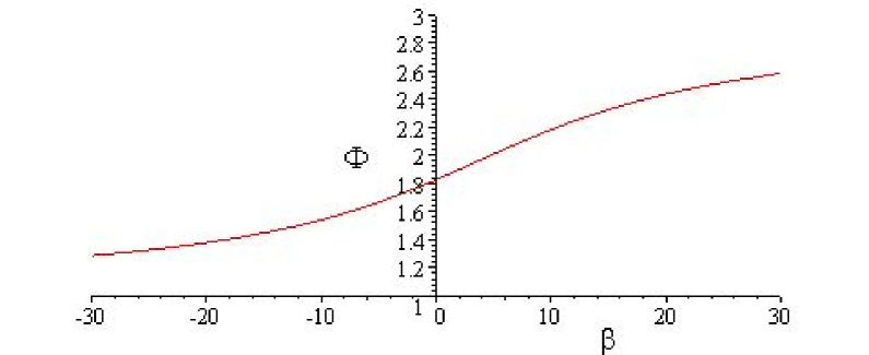
Figure 1: This figure shows the relationship between $\beta$ and $\Phi(\Phi=F(\beta)).$ Notice that as the value for $\Phi$ approaches the extremities of the outcomes, $\beta$ approaches infinity.

4.2 Numerical solutions

We will extend the econometric example by applying the above solutions to a specific problem where there are three kinds of balls labeled 1, 2 and 3. So for this problem we have $f_{1}=1,$ $f_{2}=2$ and $f_{3}=3.$ Further, we are given information regarding the average of all the boxes, $F.$ For our example this average will be, $F=2.3.$ Notice that this implies that on the average there are more $3$’s in each box. Next we take a sample of one of the boxes where $m_{1}^{\prime}=11,$ $m_{2}^{\prime}=2$ and $m_{3}^{\prime}=7.$ The numerical solution for this example is,

$$P_{\text{e}}(\theta_{1},\theta_{2})=\frac{1}{\zeta^{\prime}}e^{\beta(-2\theta_{1}-\theta_{2}+3)}\theta_{1}^{11}\theta_{2}^{2}(1-\theta_{1}-\theta_{2})^{7}~{},$$ (35)

where $\beta=14.1166$ and $\zeta^{\prime}=1874.1247.$ We show the relationship between $\beta$ and $F$ in Fig 1. The purpose of the Lagrange multiplier is to enforce the moment constraint, therefore, as $F$ goes to the extreme ($F\rightarrow 3$), $\beta\rightarrow\infty.$ This is important to mention because it graphically illustrates that whether the deviation from the sample mean is large or small, the ME method holds.

Another possible method suggested to use for this problem is the method of types EMME . This method essentially uses a form of Sanov’s theorem, which for this problem would be written as,

$$P^{\ast}(\theta_{i})=\frac{Q(\theta_{i})e^{\eta_{i}f_{i}}}{\sum_{i}Q(\theta_{i})e^{\eta_{i}f_{i}}}~{},$$ (36)

where $Q(\theta_{i})$ is ”estimated” with the frequency of the data sample. Thus $Q(\theta_{1})=\nu_{1}=11/20,$ etc. This produces the following results:

$$\theta_{t1}=0.3015,~{}\theta_{t2}=0.0971,~{}\theta_{t3}=0.6015_{.}$$ (37)

Taking the means of the ME solution yields,

$$\left\langle\theta_{1}\right\rangle=0.2942,~{}\left\langle\theta_{2}\right\rangle=0.1115,~{}\left\langle\theta_{3}\right\rangle=0.5942_{.}$$ (38)

Clearly the numerical solutions are very close, however, there are several flaws with this large deviation method. The first is that $Q$ is treated as a frequency. In the asymptotic case it would be appropriate to use a frequency, unfortunately this is not that case. The data sample is finite, $n=20.$ Another flaw is that the method does not allow for fluctuations where as the ME method does. Of course in the asymptotic case, fluctuations would be ruled out, but again, this is not the case. There is an underlying theme here: probabilities are not equivalent to frequencies except in the asymptotic case.

5 Conclusions

Using the ME method we were able to use information in the form of data and moments to update our prior probabilities. A general example was shown where the solution resembled the traditional form of Bayes rule with the standard likelihood being modified by a factor resulting from the moment constraint.

A specific econometric example was then solved in detail to illustrate the application of the method. This case can be used as a template for real world problems. Numerical results were obtained to illustrate explicitly how the method compares to other methods that are currently employed. The ME method was shown to be superior in that it did not need to make asymptotic assumptions to function and allows for fluctuations.

It must be emphasized that in the asymptotic limit, the ME form is analogous to Sanov’s theorem. However, this is only one special case. The ME method is more robust in that it can also be used to solve traditional Bayesian problems. In fact it was shown that if there is no moment constraint, one recovers Bayes rule.

Therefore, we would like to emphasize that anything one can do with Bayes, one can now do with ME. Additionally, in ME one now has the ability to apply additional information that Bayesian methods could not. Further, any work done with Bayesian techniques can be implemented into the ME method directly through the joint prior. Finally the ME method can now also be used to solve ill-posed problems in econometrics.

Acknowledgements: We would like to acknowledge valuable discussions with A. Caticha, M. Grendar and C. Rodríguez.

References

- (1) E. T. Jaynes, Phys. Rev. 106, 620 and 108, 171 (1957); R. D. Rosenkrantz (ed.), E. T. Jaynes: Papers on Probability, Statistics and Statistical Physics (Reidel, Dordrecht, 1983); E. T. Jaynes, Probability Theory: The Logic of Science (Cambridge University Press, Cambridge, 2003).
- (2) J. E. Shore and R. W. Johnson, IEEE Trans. Inf. Theory IT-26, 26 (1980); IEEE Trans. Inf. Theory IT-27, 26 (1981).
- (3) J. Skilling, “The Axioms of Maximum Entropy”, Maximum-Entropy and Bayesian Methods in Science and Engineering, G. J. Erickson and C. R. Smith (eds.) (Kluwer, Dordrecht, 1988).
- (4) A. Caticha and A. Giffin, “Updating Probabilities”, Bayesian Inference and Maximum Entropy Methods in Science and Engineering, ed. by Ali Mohammad-Djafari (ed.), AIP Conf. Proc. 872, 31 (2006) (http://arxiv.org/abs/physics/0608185).
- (5) A. Giffin and A. Caticha, “Updating Probabilities with Data and Moments”, to be published in Bayesian Inference and Maximum Entropy Methods in Science and Engineering, AIP Conf. Proc. (2007).
- (6) T. M. Cover and J. A. Thomas, Elements of Information Theory - 2nd Ed. (Wiley, New York 2006).
- (7) M. Grendar and G. Judge, ”Large Deviations Theory and Empirical Estimator Choice”, Department of Agricultural & Resource Economics, UCB. CUDARE Working Paper 1012.